Embed Size (px)
Citation preview
Mutliple Antennas• Multi-Antennas so far:- Provide diversity gain and increase reliability- Provide power gain via beamforming (Rx, Tx, opportunistic)
• But no degrees of freedom (DoF) gain- because at high SNR the capacity curves have the same slope- DoF gain is more significant in the high SNR regime
• MIMO channels have a potential to provide DoF gain by spatially multiplexing multiple data streams
• Key questions: - How the spatial multiplexing capability depends on the physical
environment?- How to establish statistical models that capture the properties
succinctly?
2
Plot• First study the spatial multiplexing capability of MIMO:- Convert a MIMO channel to parallel channel via SVD- Identify key factors for DoF gain: rank and condition number
• Then explore physical modeling of MIMO with examples:- Angular resolvability- Multipath provides DoF gain
• Finally study statistical modeling of MIMO channels:- Spatial domain vs. angular domain- Analogy with time-frequency channel modeling (Lecture 1)
3
Outline• Spatial multiplexing capability of MIMO systems
• Physical modeling of MIMO channels
• Statistical modeling of MIMO channels
4

5
Spatial Multiplexing in MIMO Systems
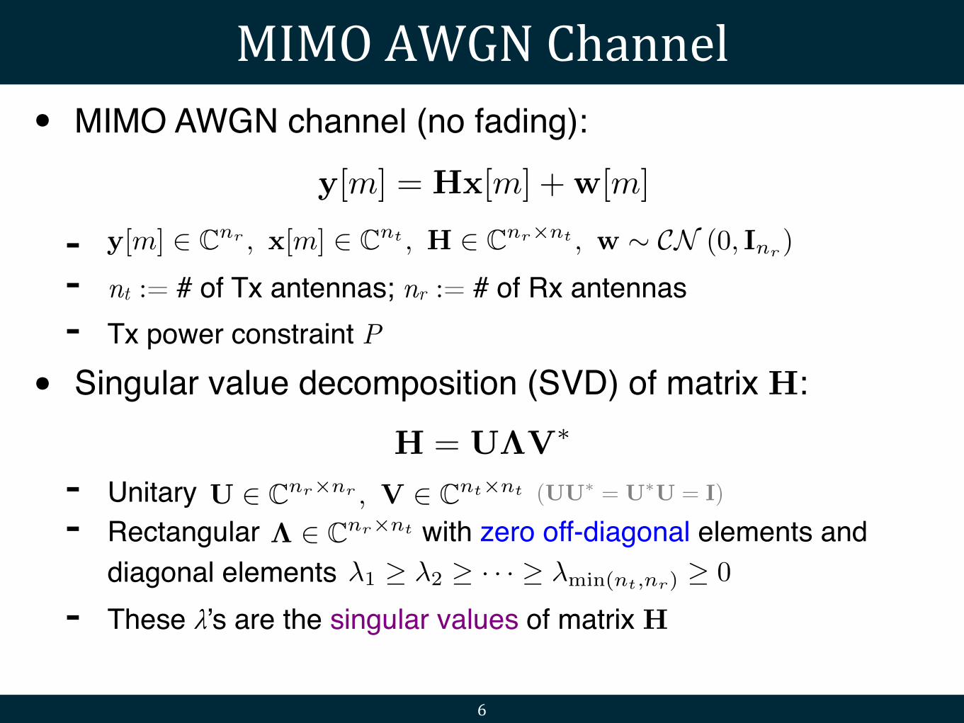
MIMO AWGN Channel• MIMO AWGN channel (no fading):
- - nt := # of Tx antennas; nr := # of Rx antennas- Tx power constraint P
• Singular value decomposition (SVD) of matrix H:
- Unitary- Rectangular !! ! ! with zero off-diagonal elements and
diagonal elements - These λ’s are the singular values of matrix H
6
y[m] = Hx[m] +w[m]
y[m] 2 Cnr , x[m] 2 Cnt , H 2 Cnr⇥nt , w ⇠ CN (0, Inr )
H = U⇤V⇤
U 2 Cnr⇥nr , V 2 Cnt⇥nt (UU⇤ = U⇤U = I)
⇤ 2 Cnr⇥nt
�1 � �2 � · · · � �min(nt,nr) � 0

MIMO Capacity via SVD• Change of coordinate:
- Let ! ! ! ! ! ! ! ! ! ! , get an equivalent channel
- Power of x and w are preserved since U and V are unitary
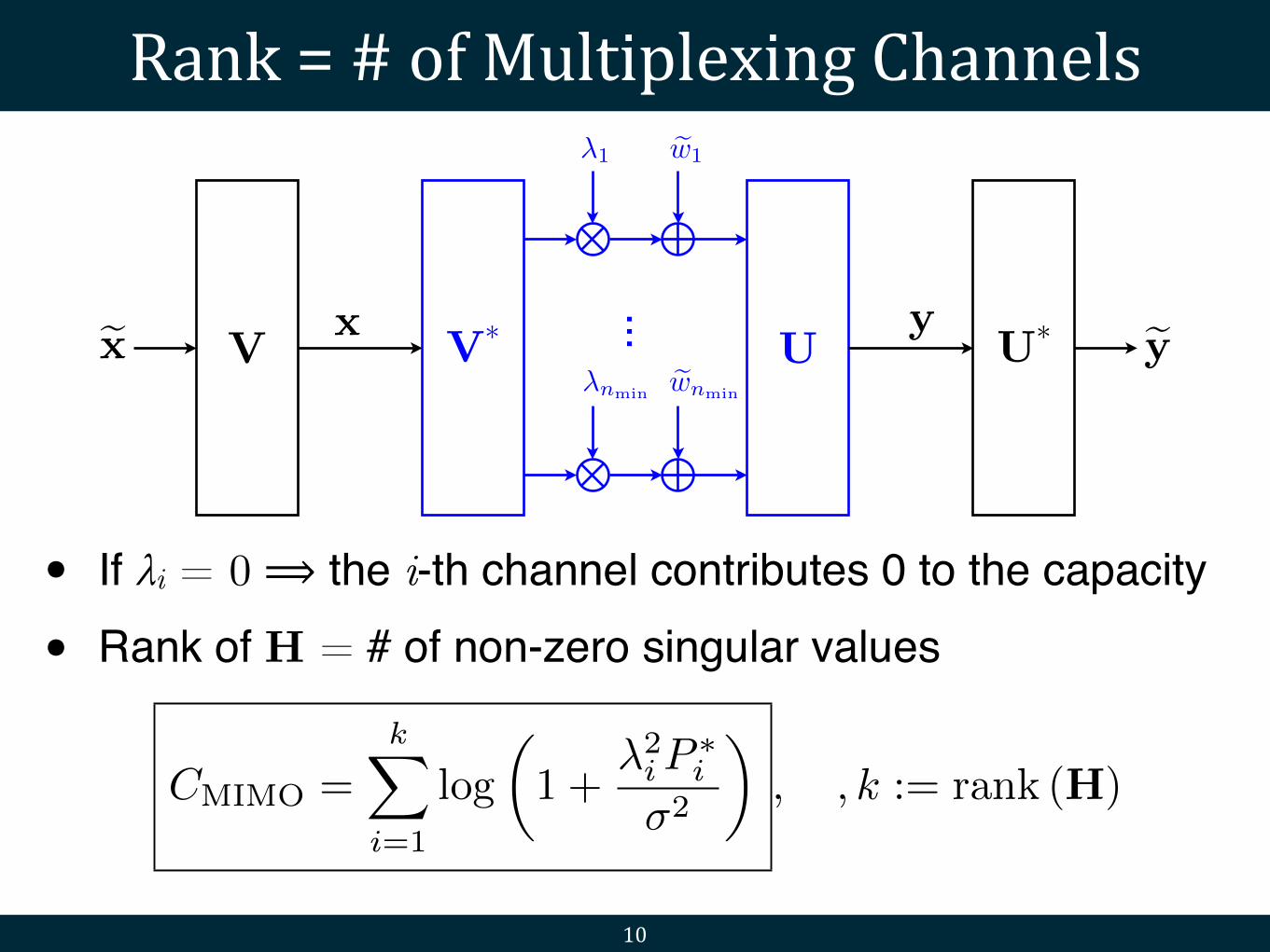
• Parallel channel: since the off-diagonal entries of Λ are all zero, the above vector channel consists of nmin := min{nt,nr} parallel channels:
- Capacity can be found via water-filling
7
ey := U
⇤y, e
x := V
⇤x, e
w := U
⇤w
y = Hx+w = U⇤V⇤x+w () U
⇤y = ⇤V
⇤x+U
⇤w
ey = ⇤
ex+ e
w
eyi = �iexi + ewi, i = 1, 2, . . . , nmin
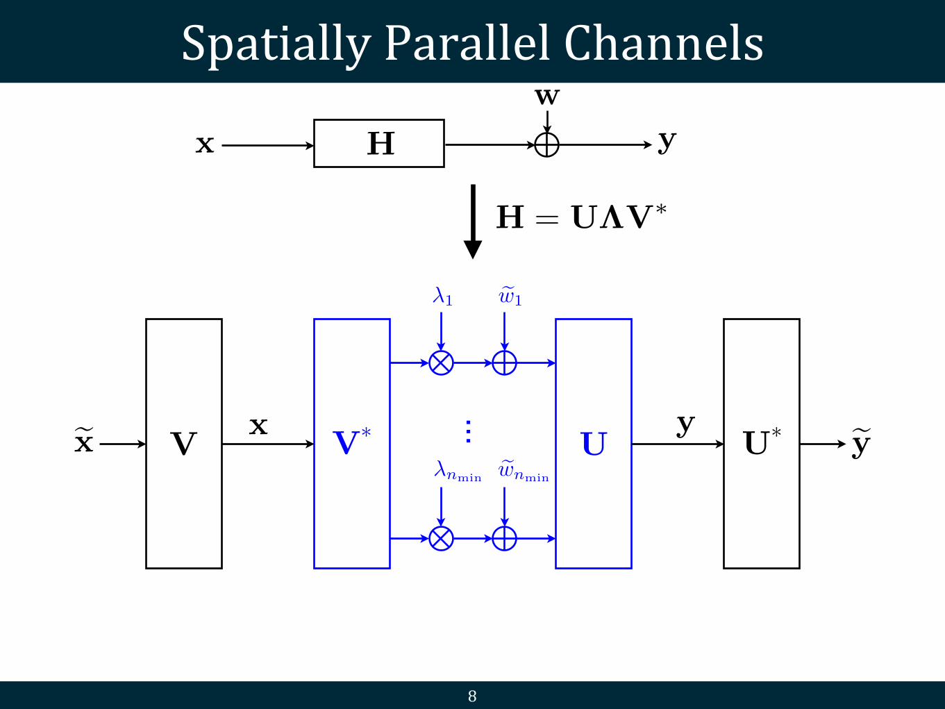
Spatially Parallel Channels
8
V* ...
�1
�nmin ewnmin
ew1
Ux
yV U* eye
x
x
yH
w
H = U⇤V⇤

Multiplexing over Parallel Channels
9
294 MIMO I: spatial multiplexing and channel modeling
+
AWGNcoder
AWGNcoder
{x1[m]}~ {y1 [m]}~
{xnmin[m]}~ {ynmin[m]}~
.
.
.
.
.
.
.
.
.
n min information
streams
{0}
{0}
{w[m]}
U*HV
Decoder
Decoder
There is a clear analogy between this architecture and the OFDM systemFigure 7.2 The SVD architecturefor MIMO communication. introduced in Chapter 3. In both cases, a transformation is applied to convert a
matrix channel into a set of parallel independent sub-channels. In the OFDMsetting, the matrix channel is given by the circulant matrix C in (3.139),defined by the ISI channel together with the cyclic prefix added onto theinput symbols. In fact, the decomposition C=Q−1!Q in (3.143) is the SVDdecomposition of a circulant matrix C, with U = Q−1 and V∗ = Q. Theimportant difference between the ISI channel and the MIMO channel is that,for the former, the U and V matrices (DFTs) do not depend on the specificrealization of the ISI channel, while for the latter, they do depend on thespecific realization of the MIMO channel.
7.1.2 Rank and condition number
What are the key parameters that determine performance? It is simpler tofocus separately on the high and the low SNR regimes. At high SNR, thewater level is deep and the policy of allocating equal amounts of power onthe non-zero eigenmodes is asymptotically optimal (cf. Figure 5.24(a)):
C ≈k!
i=1
log"1+ P"2
i
kN0
#≈ k log SNR+
k!
i=1
log""2i
k
#bits/s/Hz# (7.12)
where k is the number of non-zero "2i , i.e., the rank of H, and SNR $= P/N0.
The parameter k is the number of spatial degrees of freedom per second perhertz. It represents the dimension of the transmitted signal as modified bythe MIMO channel, i.e., the dimension of the image of H. This is equal tothe rank of the matrix H and with full rank, we see that a MIMO channelprovides nmin spatial degrees of freedom.
P ⇤i =
✓⌫ � �2
�2i
◆+
, ⌫ satisfiesnminX
i=1
P ⇤i = PCMIMO =
nminX
i=1
log
✓1 +
�2iP
⇤i
�2
◆
Rank = # of Multiplexing Channels
10
V* ...
�1
�nmin ewnmin
ew1
Ux
yV U* eye
x
• If λi = 0 ⟹ the i-th channel contributes 0 to the capacity
• Rank of H = # of non-zero singular values
CMIMO =
kX
i=1
log
✓1 +
�2iP
⇤i
�2
◆, , k := rank (H)
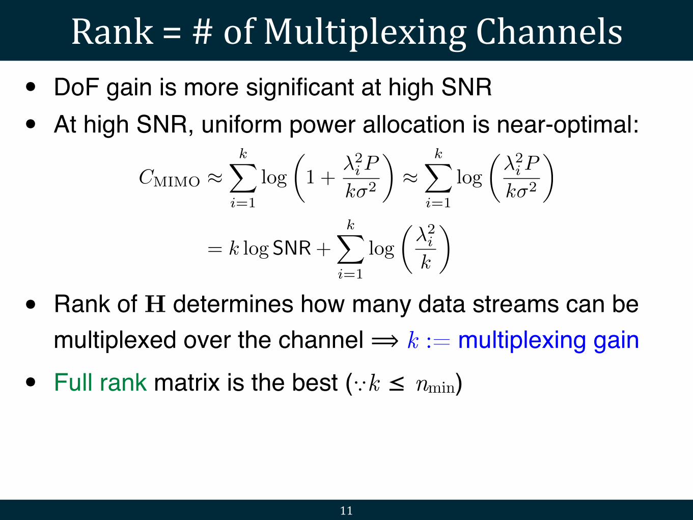
Rank = # of Multiplexing Channels• DoF gain is more significant at high SNR• At high SNR, uniform power allocation is near-optimal:
• Rank of H determines how many data streams can be multiplexed over the channel ⟹ k := multiplexing gain
• Full rank matrix is the best (∵k ≤ nmin)
11
CMIMO ⇡kX
i=1
log
✓1 +
�2iP
k�2
◆⇡
kX
i=1
log
✓�2iP
k�2
◆
= k log SNR+
kX
i=1
log
✓�2i
k
◆
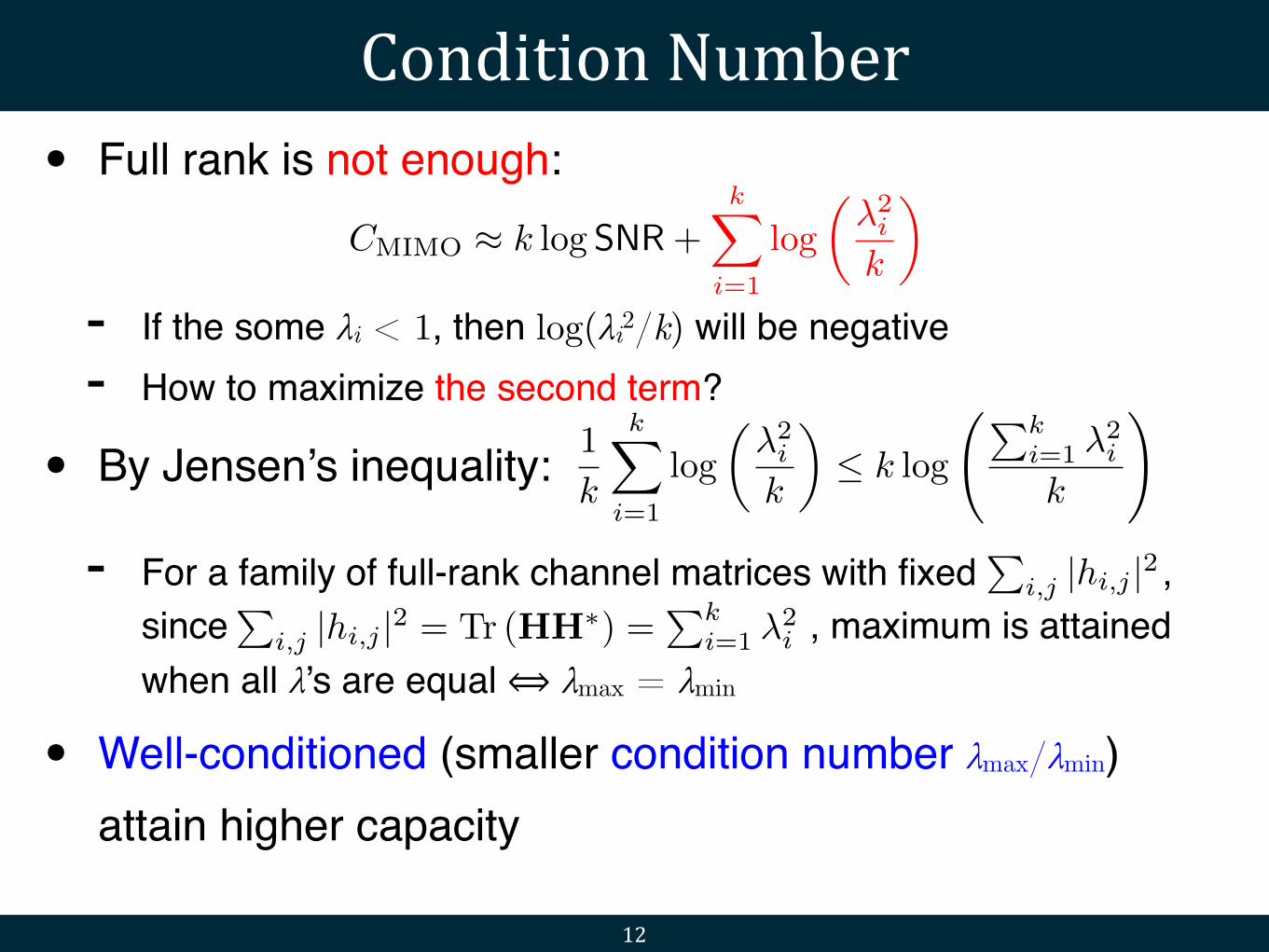
Condition Number• Full rank is not enough:
- If the some λi < 1, then log(λi2/k) will be negative- How to maximize the second term?
• By Jensen’s inequality:
- For a family of full-rank channel matrices with fixed ! ! ! , since!! ! ! ! ! ! ! ! ! ! , maximum is attained when all λ’s are equal ⟺ λmax = λmin
• Well-conditioned (smaller condition number λmax/λmin) attain higher capacity
12
CMIMO ⇡ k log SNR+
kX
i=1
log
✓�2i
k
◆
1
k
kX
i=1
log
✓�2i
k
◆ k log
Pki=1 �
2i
k
!
Pi,j |hi,j |2P
i,j |hi,j |2 = Tr (HH⇤) =Pk
i=1 �2i
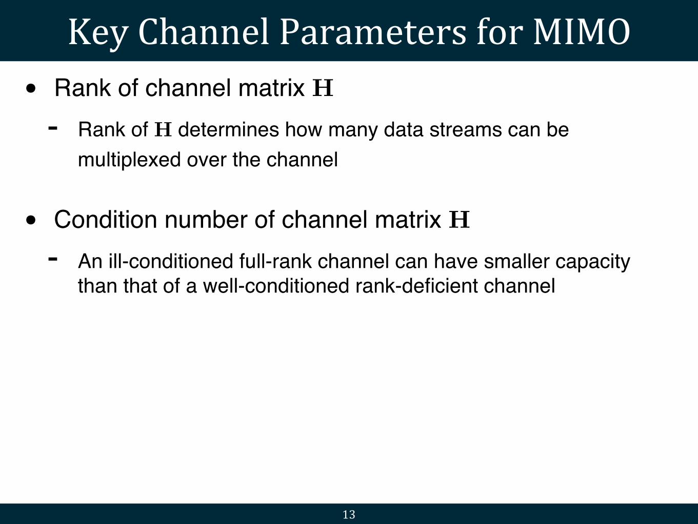
Key Channel Parameters for MIMO• Rank of channel matrix H- Rank of H determines how many data streams can be
multiplexed over the channel
• Condition number of channel matrix H- An ill-conditioned full-rank channel can have smaller capacity
than that of a well-conditioned rank-deficient channel
13
14
Physical Modeling of MIMO Channels
15
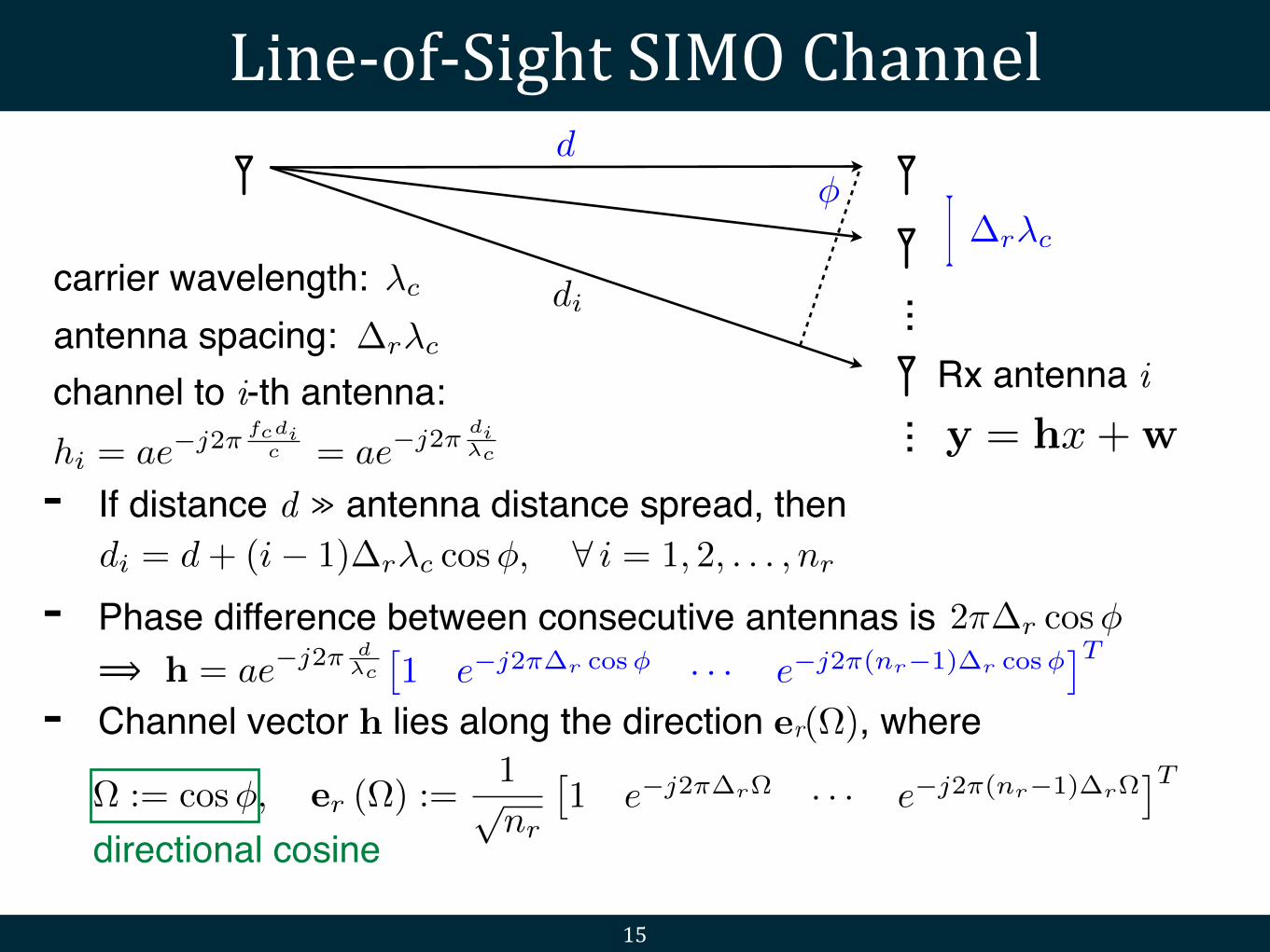
Line-‐of-‐Sight SIMO Channel
...
�d
�r�c
carrier wavelength: �c
antenna spacing: �r�c
- If distance d ≫ antenna distance spread, then
- Phase difference between consecutive antennas is- ⟹ - Channel vector h lies along the direction er(Ω), where
Rx antenna i
...
di
2⇡�r cos�
hi = ae�j2⇡fcdi
c = ae�j2⇡di�c
channel to i-th antenna:
di = d+ (i� 1)�r�c cos�, 8 i = 1, 2, . . . , nr
h = ae�j2⇡ d�c
⇥1 e�j2⇡�r cos� · · · e�j2⇡(nr�1)�r cos�
⇤T
⌦ := cos�, er (⌦) :=1
pnr
⇥1 e�j2⇡�r⌦ · · · e�j2⇡(nr�1)�r⌦
⇤T
directional cosine
y = hx+w
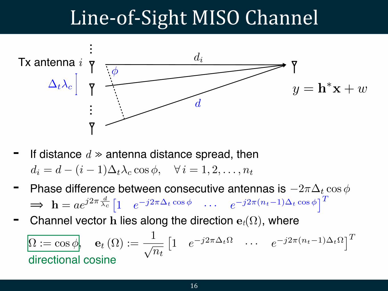
- If distance d ≫ antenna distance spread, then
- Phase difference between consecutive antennas is- ⟹ - Channel vector h lies along the direction et(Ω), where
di = d� (i� 1)�t�c cos�, 8 i = 1, 2, . . . , nt
16
Line-‐of-‐Sight MISO Channel
�
d
Tx antenna i
...
... di
directional cosine
�t�c y = h
⇤x+ w
�2⇡�t cos�
h = aej2⇡d�c
⇥1 e�j2⇡�t cos� · · · e�j2⇡(nt�1)�t cos�
⇤T
⌦ := cos�, et (⌦) :=1
pnt
⇥1 e�j2⇡�t⌦ · · · e�j2⇡(nt�1)�t⌦
⇤T

Line-‐of-‐Sight SIMO and MISO• Line-of-sight SIMO:- y = hx+w, h is along the receive spatial signature er(Ω), where
- nr -fold power gain, no DoF gain
• Line-of-sight SIMO:- y = hx+w, h is along the transmit spatial signature et(Ω), where
- nt -fold power gain, no DoF gain
17
er (⌦) :=1
pnr
⇥1 e�j2⇡�r⌦ · · · e�j2⇡(nr�1)�r⌦
⇤T
et (⌦) :=1
pnt
⇥1 e�j2⇡�t⌦ · · · e�j2⇡(nt�1)�t⌦
⇤T
...
18
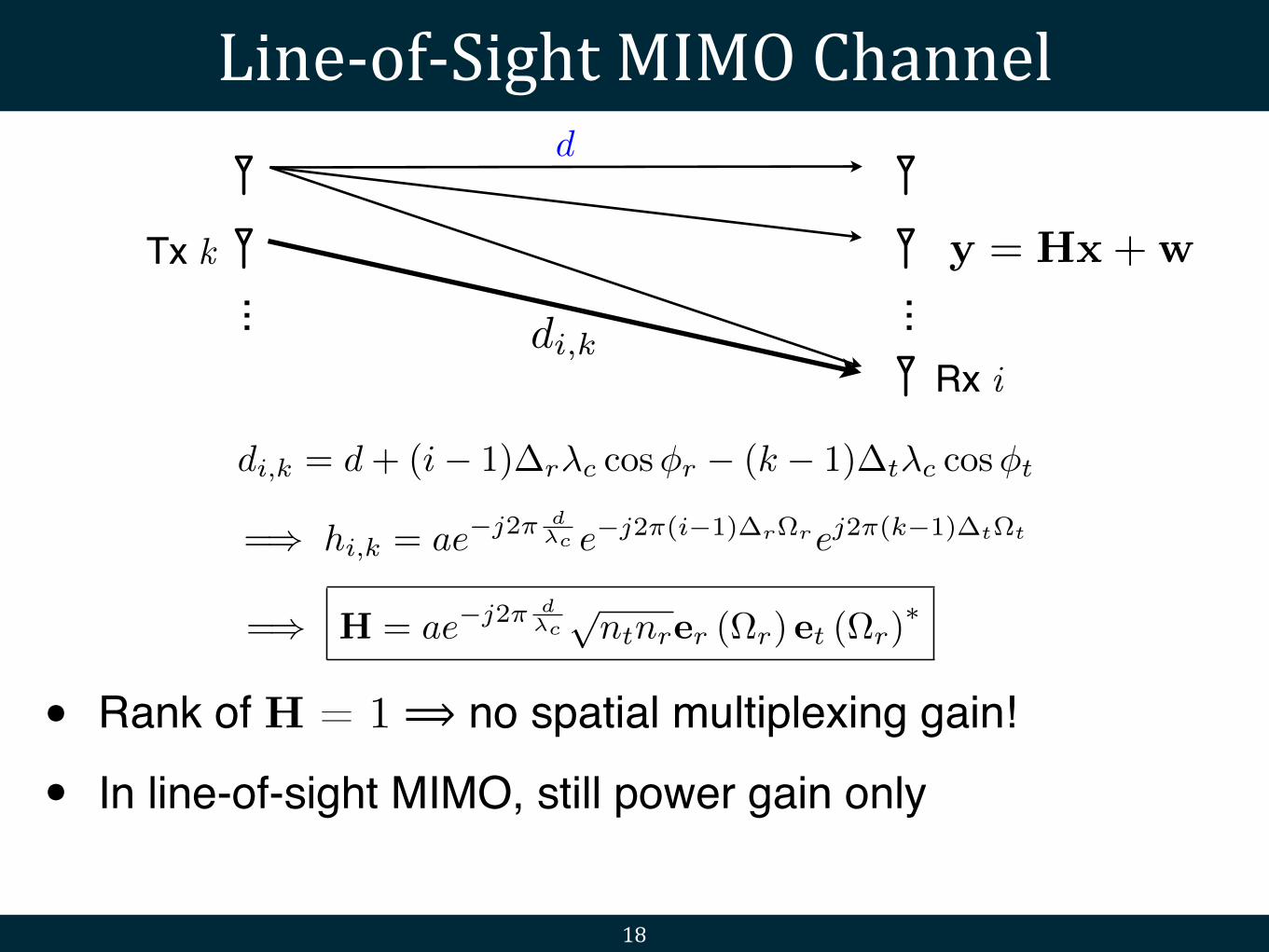
Line-‐of-‐Sight MIMO Channeld
...
y = Hx+wTx k
Rx idi,k
=) hi,k = ae�j2⇡ d�c e�j2⇡(i�1)�r⌦rej2⇡(k�1)�t⌦t
di,k = d+ (i� 1)�r�c cos�r � (k � 1)�t�c cos�t
=) H = ae�j2⇡ d�cpntnrer (⌦r) et (⌦r)
⇤
• Rank of H = 1 ⟹ no spatial multiplexing gain!
• In line-of-sight MIMO, still power gain only