Lecture 13: Review Session,

and New Keynesian Model

ECO 503: Macroeconomic Theory I

Benjamin Moll

Princeton University

Fall 2014

1 / 30

Review of Material

• Course had two components

1 tools

2 substance

• Let’s go over these, emphasizing what I want you to takeaway from this course

2 / 30

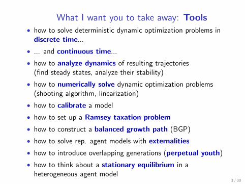
What I want you to take away: Tools

• how to solve deterministic dynamic optimization problems indiscrete time...

• ... and continuous time...

• how to analyze dynamics of resulting trajectories(find steady states, analyze their stability)

• how to numerically solve dynamic optimization problems(shooting algorithm, linearization)

• how to calibrate a model

• how to set up a Ramsey taxation problem

• how to construct a balanced growth path (BGP)

• how to solve rep. agent models with externalities

• how to introduce overlapping generations (perpetual youth)

• how to think about a stationary equilibrium in aheterogeneous agent model

3 / 30

What I want you to take away:

Substance

• Basic tradeoffs in growth model

• Income vs. substitution effects

• Effects of response to unexpected productivity increase ingrowth model (building block of business cycle model)

• Quick convergence of growth model to steady state (or BGP)

• Kaldor facts (and caveats)

• Growth model = decent model of growth experience of U.S.(and other developed countries)...

• ... but bad model of “development dynamics”

4 / 30

What I want you to take away:

Substance

• Ramsey taxation of capital:

• robust prediction: if possible, want to tax more today thantomorrow

• not robust: ⇒ zero capital taxes in long-run

• Endogenous growth: all theories make some linearityassumption

• if it doesn’t jump out at you, it’s hidden somewhere

• Upper tails of income and wealth distribution follow Paretodistributions

• Q: where do Pareto distributions come from?A: simplest mechanism: combination of

1 exponential growth

2 random death (exponentially distributed)

5 / 30

New Keynesian Model

• New Keynesian model = RBC/growth model with sticky prices

• References:

• Gali (2008): most accessible intro

• Woodford (2003): New Keynesian bible

• Clarida, Gali and Gertler (1999): most influential article

• Gali and Monacelli (2005): small open economy version

6 / 30

Why Should You Care?

• Simple framework to think about relationship between

monetary policy, inflation and the business cycle.

• RBC model: cannot even think about these issues! Real

variables are completely separate from nominal variables

(“monetary neutrality”, “classical dichotomy”).

• Corollary: monetary policy has no effect on any real variables.

• Sticky prices break “monetary neutrality”

• Workhorse model at central banks (see Fed presentation

/DB_ECO521_2012_2013/LectureNotes/MacroModelsAtTheFed.pdf)

• Makes some sense of newspaper statements like: “a boom

leads the economy to overheat and creates inflationary

pressure”

• Some reason to believe that “demand shocks” (e.g. consumer

confidence, animal spirits) may drive business cycle. Sticky

prices = one way to get this story off the ground.7 / 30

Outline

(1) Model with flexible prices

(2) Model with sticky prices

8 / 30

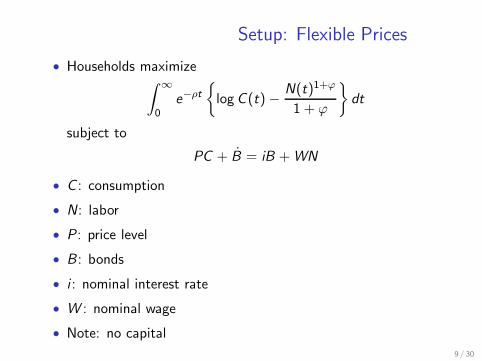
Setup: Flexible Prices

• Households maximize∫ ∞

0e−ρt

{

logC (t)−N(t)1+ϕ

1 + ϕ

}

dt

subject to

PC + B = iB +WN

• C : consumption

• N: labor

• P : price level

• B : bonds

• i : nominal interest rate

• W : nominal wage

• Note: no capital

9 / 30

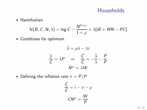
Households

• Hamiltonian

H(B ,C ,N, λ) = logC −N1+ϕ

1 + ϕ+ λ[iB +WN − PC ]

• Conditions for optimum

λ = ρλ− λi

1

C= λP ⇒

C

C= −

λ

λ−

P

P

Nϕ = λW

• Defining the inflation rate π = P/P

C

C= i − π − ρ

CNϕ =W

P10 / 30

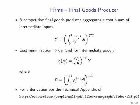
Firms – Final Goods Producer

• A competitive final goods producer aggregates a continuum of

intermediate inputs

Y =

(∫ 1

0y

ε−1ε

j dj

)

ε

ε−1

• Cost minimization ⇒ demand for intermediate good j

yj(pj ) =(pj

P

)−ε

Y

where

P =

(∫ 1

0p1−ε

j dj

)

11−ε

• For a derivation see the Technical Appendix of

http://www.crei.cat/people/gali/pdf_files/monograph/slides-ch3.pdf

11 / 30

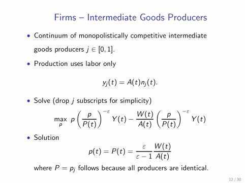
Firms – Intermediate Goods Producers

• Continuum of monopolistically competitive intermediate

goods producers j ∈ [0, 1].

• Production uses labor only

yj(t) = A(t)nj(t).

• Solve (drop j subscripts for simplicity)

maxp

p

(

p

P(t)

)−ε

Y (t)−W (t)

A(t)

(

p

P(t)

)−ε

Y (t)

• Solution

p(t) = P(t) =ε

ε− 1

W (t)

A(t)

where P = pj follows because all producers are identical.

12 / 30

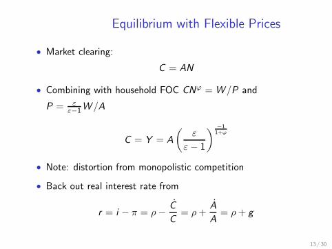
Equilibrium with Flexible Prices

• Market clearing:

C = AN

• Combining with household FOC CNϕ = W /P and

P = ε

ε−1W /A

C = Y = A

(

ε

ε− 1

)−11+ϕ

• Note: distortion from monopolistic competition

• Back out real interest rate from

r = i − π = ρ−C

C= ρ+

A

A= ρ+ g

13 / 30

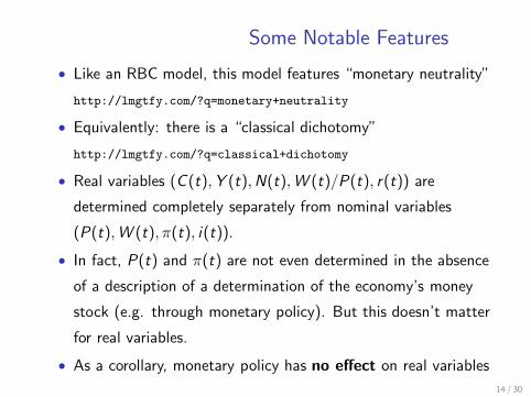
Some Notable Features

• Like an RBC model, this model features “monetary neutrality”

http://lmgtfy.com/?q=monetary+neutrality

• Equivalently: there is a “classical dichotomy”

http://lmgtfy.com/?q=classical+dichotomy

• Real variables (C (t),Y (t),N(t),W (t)/P(t), r(t)) are

determined completely separately from nominal variables

(P(t),W (t), π(t), i(t)).

• In fact, P(t) and π(t) are not even determined in the absence

of a description of a determination of the economy’s money

stock (e.g. through monetary policy). But this doesn’t matter

for real variables.

• As a corollary, monetary policy has no effect on real variables

14 / 30

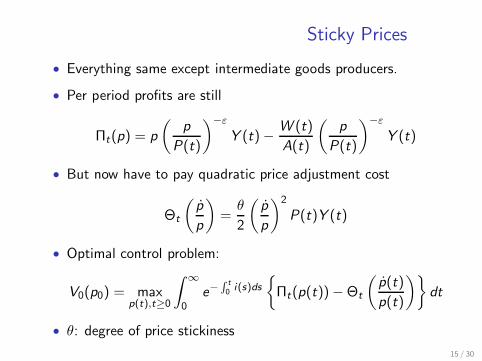
Sticky Prices

• Everything same except intermediate goods producers.

• Per period profits are still

Πt(p) = p

(

p

P(t)

)−ε

Y (t)−W (t)

A(t)

(

p

P(t)

)−ε

Y (t)

• But now have to pay quadratic price adjustment cost

Θt

(

p

p

)

=θ

2

(

p

p

)2

P(t)Y (t)

• Optimal control problem:

V0(p0) = maxp(t),t≥0

∫ ∞

0e−

∫ t

0i(s)ds

{

Πt(p(t))−Θt

(

p(t)

p(t)

)}

dt

• θ: degree of price stickiness

15 / 30

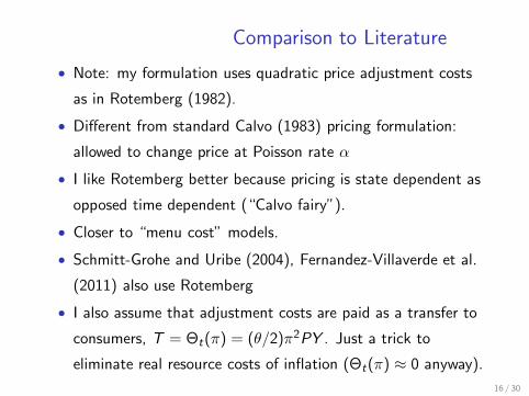
Comparison to Literature

• Note: my formulation uses quadratic price adjustment costs

as in Rotemberg (1982).

• Different from standard Calvo (1983) pricing formulation:

allowed to change price at Poisson rate α

• I like Rotemberg better because pricing is state dependent as

opposed time dependent (“Calvo fairy”).

• Closer to “menu cost” models.

• Schmitt-Grohe and Uribe (2004), Fernandez-Villaverde et al.

(2011) also use Rotemberg

• I also assume that adjustment costs are paid as a transfer to

consumers, T = Θt(π) = (θ/2)π2PY . Just a trick to

eliminate real resource costs of inflation (Θt(π) ≈ 0 anyway).

16 / 30

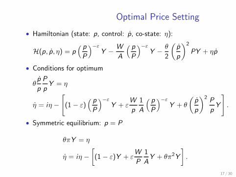
Optimal Price Setting

• Hamiltonian (state: p, control: p, co-state: η):

H(p, p, η) = p( p

P

)−ε

Y −W

A

( p

P

)−ε

Y −θ

2

(

p

p

)2

PY + ηp

• Conditions for optimum

θp

p

P

pY = η

η = iη −

[

(1− ε)( p

P

)−ε

Y + εW

p

1

A

( p

P

)−ε

Y + θ

(

p

p

)2P

pY

]

.

• Symmetric equilibrium: p = P

θπY = η

η = iη −

[

(1− ε)Y + εW

P

1

AY + θπ2Y

]

.

17 / 30

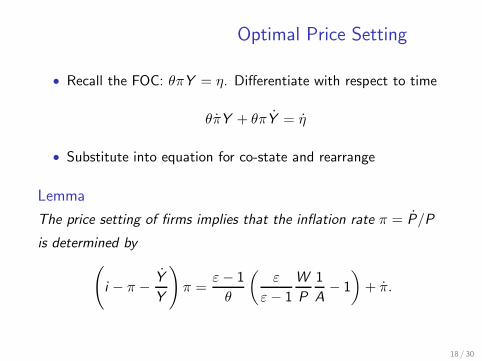
Optimal Price Setting

• Recall the FOC: θπY = η. Differentiate with respect to time

θπY + θπY = η

• Substitute into equation for co-state and rearrange

Lemma

The price setting of firms implies that the inflation rate π = P/P

is determined by

(

i − π −Y

Y

)

π =ε− 1

θ

(

ε

ε− 1

W

P

1

A− 1

)

+ π.

18 / 30

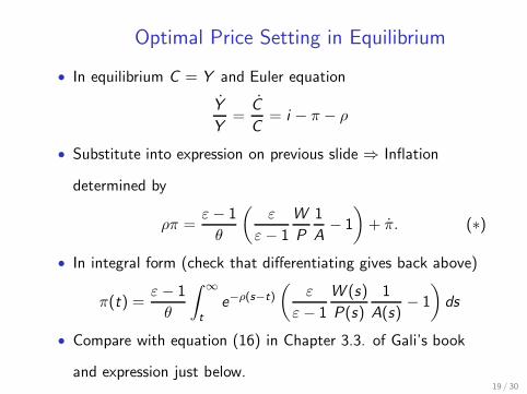
Optimal Price Setting in Equilibrium

• In equilibrium C = Y and Euler equation

Y

Y=

C

C= i − π − ρ

• Substitute into expression on previous slide ⇒ Inflation

determined by

ρπ =ε− 1

θ

(

ε

ε− 1

W

P

1

A− 1

)

+ π. (∗)

• In integral form (check that differentiating gives back above)

π(t) =ε− 1

θ

∫ ∞

t

e−ρ(s−t)

(

ε

ε− 1

W (s)

P(s)

1

A(s)− 1

)

ds

• Compare with equation (16) in Chapter 3.3. of Gali’s book

and expression just below.19 / 30

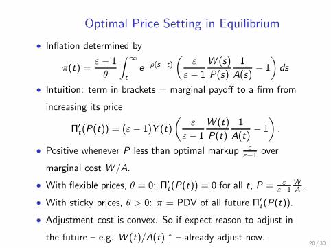
Optimal Price Setting in Equilibrium

• Inflation determined by

π(t) =ε− 1

θ

∫ ∞

t

e−ρ(s−t)

(

ε

ε− 1

W (s)

P(s)

1

A(s)− 1

)

ds

• Intuition: term in brackets = marginal payoff to a firm from

increasing its price

Π′t(P(t)) = (ε− 1)Y (t)

(

ε

ε− 1

W (t)

P(t)

1

A(t)− 1

)

.

• Positive whenever P less than optimal markup ε

ε−1 over

marginal cost W /A.

• With flexible prices, θ = 0: Π′t(P(t)) = 0 for all t, P = ε

ε−1WA.

• With sticky prices, θ > 0: π = PDV of all future Π′t(P(t)).

• Adjustment cost is convex. So if expect reason to adjust in

the future – e.g. W (t)/A(t) ↑ – already adjust now.20 / 30

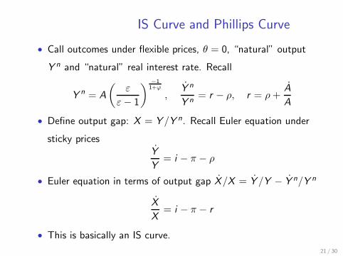
IS Curve and Phillips Curve

• Call outcomes under flexible prices, θ = 0, “natural” output

Y n and “natural” real interest rate. Recall

Y n = A

(

ε

ε− 1

)−11+ϕ

,Y n

Y n= r − ρ, r = ρ+

A

A

• Define output gap: X = Y /Y n. Recall Euler equation under

sticky pricesY

Y= i − π − ρ

• Euler equation in terms of output gap X/X = Y /Y − Y n/Y n

X

X= i − π − r

• This is basically an IS curve.

21 / 30

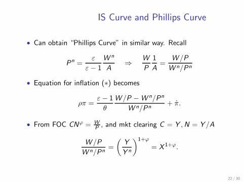
IS Curve and Phillips Curve

• Can obtain “Phillips Curve” in similar way. Recall

Pn =ε

ε− 1

W n

A⇒

W

P

1

A=

W /P

W n/Pn

• Equation for inflation (∗) becomes

ρπ =ε− 1

θ

W /P −W n/Pn

W n/Pn+ π.

• From FOC CNϕ = WP, and mkt clearing C = Y ,N = Y /A

W /P

W n/Pn=

(

Y

Y n

)1+ϕ

= X 1+ϕ.

22 / 30

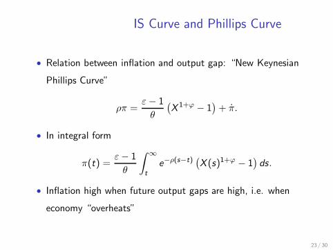
IS Curve and Phillips Curve

• Relation between inflation and output gap: “New Keynesian

Phillips Curve”

ρπ =ε− 1

θ

(

X 1+ϕ − 1)

+ π.

• In integral form

π(t) =ε− 1

θ

∫ ∞

t

e−ρ(s−t)(

X (s)1+ϕ − 1)

ds.

• Inflation high when future output gaps are high, i.e. when

economy “overheats”

23 / 30

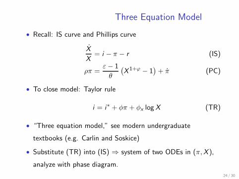
Three Equation Model

• Recall: IS curve and Phillips curve

X

X= i − π − r (IS)

ρπ =ε− 1

θ

(

X 1+ϕ − 1)

+ π (PC)

• To close model: Taylor rule

i = i∗ + φπ + φx logX (TR)

• “Three equation model,” see modern undergraduate

textbooks (e.g. Carlin and Soskice)

• Substitute (TR) into (IS) ⇒ system of two ODEs in (π,X ),

analyze with phase diagram.

24 / 30

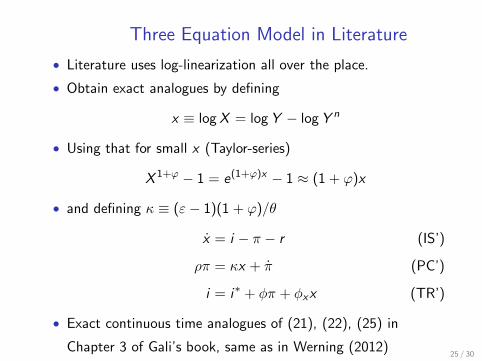
Three Equation Model in Literature

• Literature uses log-linearization all over the place.

• Obtain exact analogues by defining

x ≡ logX = logY − logY n

• Using that for small x (Taylor-series)

X 1+ϕ − 1 = e(1+ϕ)x − 1 ≈ (1 + ϕ)x

• and defining κ ≡ (ε− 1)(1 + ϕ)/θ

x = i − π − r (IS’)

ρπ = κx + π (PC’)

i = i∗ + φπ + φxx (TR’)

• Exact continuous time analogues of (21), (22), (25) in

Chapter 3 of Gali’s book, same as in Werning (2012)25 / 30

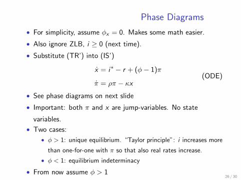
Phase Diagrams

• For simplicity, assume φx = 0. Makes some math easier.

• Also ignore ZLB, i ≥ 0 (next time).

• Substitute (TR’) into (IS’)

x = i∗ − r + (φ− 1)π

π = ρπ − κx(ODE)

• See phase diagrams on next slide

• Important: both π and x are jump-variables. No state

variables.

• Two cases:

• φ > 1: unique equilibrium. “Taylor principle”: i increases more

than one-for-one with π so that also real rates increase.

• φ < 1: equilibrium indeterminacy

• From now assume φ > 126 / 30

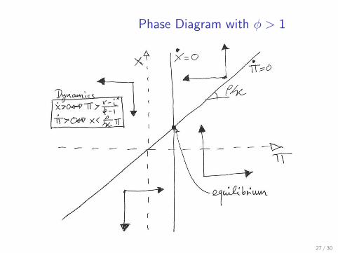
Phase Diagram with φ > 1

27 / 30

Monetary Policy

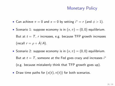
• Can achieve π = 0 and x = 0 by setting i∗ = r (and φ > 1).

• Scenario 1: suppose economy is in (x , π) = (0, 0) equilibrium.

But at t = T , r increases, e.g. because TFP growth increases

(recall r = ρ+ A/A).

• Scenario 2: suppose economy is in (x , π) = (0, 0) equilibrium.

But at t = T , someone at the Fed goes crazy and increases i∗

(e.g. because mistakenly think that TFP growth goes up).

• Draw time paths for (x(t), π(t)) for both scenarios.

28 / 30

Optimal Monetary Policy

• Huge literature

• See in particular Clarida, Gali and Gertler (1999) “The science

of monetary policy: a new Keynesian perspective”

29 / 30

Zero Lower Bound

• So far: New Keynesian 3 equation model, derived from micro

foundations

• Ignored ZLB (or “liquidity trap”), i(t) ≥ 0.

• Some references

• Eggertsson and Woodford (2003), “The zero interest-rate

bound and optimal monetary policy”

• Christiano, Eichenbaum, Rebelo (2011)“When is the

Government Spending Multiplier Large?”

• Werning (2012), “Managing a Liquidity Trap: Monetary and

Fiscal Policy”

30 / 30