lecture11 - Massachusetts Institute of Technology David&Sontag& New&York&University& Slides adapted from Luke Zettlemoyer, Carlos Guestrin, and Andrew Moore Hypotheses: decision trees

Decision trees Lecture 11

David Sontag New York University

Slides adapted from Luke Zettlemoyer, Carlos Guestrin, and Andrew Moore

Hypotheses: decision trees f : X ! Y •  Each internal node

tests an attribute xi

•  One branch for each possible attribute value xi=v

•  Each leaf assigns a class y

•  To classify input x: traverse the tree from root to leaf, output the labeled y

Cylinders

3 4 5 6 8

good bad bad Maker Horsepower

low med high america asia europe

bad bad good good good bad

Human interpretable!

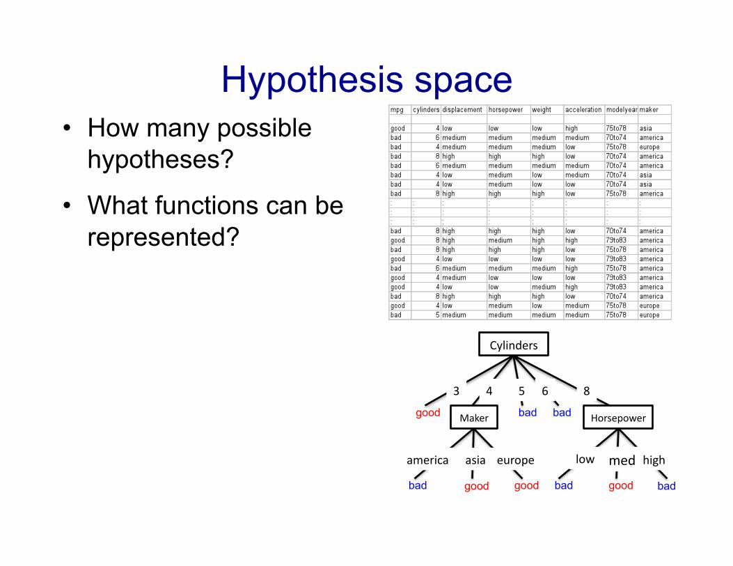
Hypothesis space •  How many possible

hypotheses?

•  What functions can be represented?

Cylinders

3 4 5 6 8




What funcGons can be represented?

•  Decision trees can represent any funcGon of the input aIributes!

•  For Boolean funcGons, path to leaf gives truth table row

•  Could require exponenGally many nodes

Expressiveness

Discrete-input, discrete-output case:– Decision trees can express any function of the input attributes.– E.g., for Boolean functions, truth table row � path to leaf:

FT

A

B

F T

B

A B A xor BF F FF T TT F TT T F

F

F F

T

T T

Continuous-input, continuous-output case:– Can approximate any function arbitrarily closely

Trivially, there is a consistent decision tree for any training setw/ one path to leaf for each example (unless f nondeterministic in x)but it probably won’t generalize to new examples

Need some kind of regularization to ensure more compact decision trees

CS194-10 Fall 2011 Lecture 8 7

(Figure from Stuart Russell)

cyl=3 ∨ (cyl=4 ∧ (maker=asia ∨ maker=europe)) ∨ …

Cylinders

3 4 5 6 8




Learning simplest decision tree is NP-‐hard

•  Learning the simplest (smallest) decision tree is an NP-‐complete problem [Hyafil & Rivest ’76]

•  Resort to a greedy heurisGc: – Start from empty decision tree – Split on next best a1ribute (feature) – Recurse

Key idea: Greedily learn trees using recursion

Take the Original Dataset..

And partition it according to the value of the attribute we split on

Records in which cylinders

= 4


= 5


= 6


= 8

Recursive Step


= 4


= 5


= 6


= 8

Build tree from These records..




Second level of tree

Recursively build a tree from the seven records in which there are four cylinders and the maker was based in Asia

(Similar recursion in the other cases)

A full tree

Spli^ng: choosing a good aIribute

X1 X2 Y T T T T F T T T T T F T F T T F F F F T F F F F

X1

Y=t : 4 Y=f : 0

t f

Y=t : 1 Y=f : 3

X2

Y=t : 3 Y=f : 1

t f

Y=t : 2 Y=f : 2

Would we prefer to split on X1 or X2?

Idea: use counts at leaves to define probability distributions, so we can measure uncertainty!

Measuring uncertainty

•  Good split if we are more certain about classificaGon a_er split – DeterminisGc good (all true or all false) – Uniform distribuGon bad – What about distribuGons in between?

P(Y=A) = 1/4 P(Y=B) = 1/4 P(Y=C) = 1/4 P(Y=D) = 1/4

P(Y=A) = 1/2 P(Y=B) = 1/4 P(Y=C) = 1/8 P(Y=D) = 1/8

Entropy Entropy H(Y) of a random variable Y

More uncertainty, more entropy!

Information Theory interpretation: H(Y) is the expected number of bits needed to encode a randomly drawn value of Y (under most efficient code)

Probability of heads

Entrop

y

Entropy of a coin flip

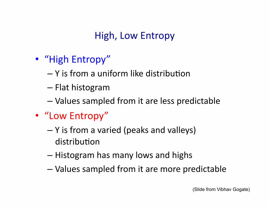
High, Low Entropy

•  “High Entropy” – Y is from a uniform like distribuGon

– Flat histogram – Values sampled from it are less predictable

•  “Low Entropy” – Y is from a varied (peaks and valleys) distribuGon

– Histogram has many lows and highs

– Values sampled from it are more predictable

(Slide from Vibhav Gogate)

Entropy Example

X1 X2 Y T T T T F T T T T T F T F T T F F F

P(Y=t) = 5/6 P(Y=f) = 1/6

H(Y) = - 5/6 log2 5/6 - 1/6 log2 1/6 = 0.65

Probability of heads

Entrop

y

Entropy of a coin flip

CondiGonal Entropy CondiGonal Entropy H( Y |X) of a random variable Y condiGoned on a

random variable X

X1

Y=t : 4 Y=f : 0

t f

Y=t : 1 Y=f : 1

P(X1=t) = 4/6 P(X1=f) = 2/6


Example:

H(Y|X1) = - 4/6 (1 log2 1 + 0 log2 0) - 2/6 (1/2 log2 1/2 + 1/2 log2 1/2) = 2/6

InformaGon gain •  Decrease in entropy (uncertainty) a_er spli^ng


In our running example:

IG(X1) = H(Y) – H(Y|X1) = 0.65 – 0.33

IG(X1) > 0 ! we prefer the split!

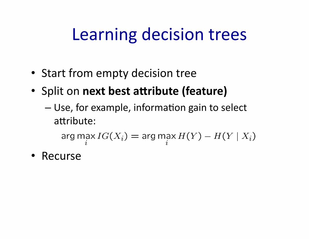
Learning decision trees

•  Start from empty decision tree •  Split on next best a1ribute (feature)

– Use, for example, informaGon gain to select aIribute:

•  Recurse

When to stop?

First split looks good! But, when do we stop?

Base Case One

Don’t split a node if all matching

records have the same

output value

Base Case Two

Don’t split a node if data points are

identical on remaining attributes

Base Cases: An idea

•  Base Case One: If all records in current data subset have the same output then don’t recurse

•  Base Case Two: If all records have exactly the same set of input aIributes then don’t recurse

Proposed Base Case 3: If all attributes have small information gain then don’t

recurse

• This is not a good idea

The problem with proposed case 3

y = a XOR b

The information gains:

If we omit proposed case 3:

y = a XOR b The resulting decision tree:

Instead, perform pruning after building a tree

Decision trees will overfit

Decision trees will overfit

•  Standard decision trees have no learning bias – Training set error is always zero!

•  (If there is no label noise) – Lots of variance – Must introduce some bias towards simpler trees

•  Many strategies for picking simpler trees – Fixed depth – Minimum number of samples per leaf

•  Random forests

Real-‐Valued inputs

What should we do if some of the inputs are real-‐valued?

Infinite number of possible split values!!!

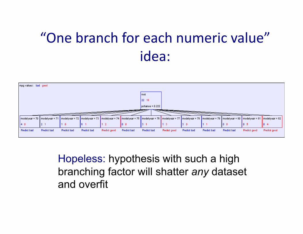
“One branch for each numeric value” idea:

Hopeless: hypothesis with such a high branching factor will shatter any dataset and overfit

Threshold splits

•  Binary tree: split on aIribute X at value t

– One branch: X < t – Other branch: X ≥ t

Year

<78 ≥78

good bad

•  Requires small change •  Allow repeated splits on same

variable along a path

Year

<70 ≥70

good bad

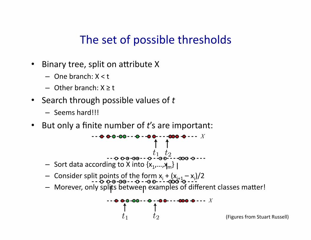
The set of possible thresholds

•  Binary tree, split on aIribute X –  One branch: X < t –  Other branch: X ≥ t

•  Search through possible values of t –  Seems hard!!!

•  But only a finite number of t’s are important:

–  Sort data according to X into {x1,…,xm} –  Consider split points of the form xi + (xi+1 – xi)/2

–  Morever, only splits between examples of different classes maIer!

(Figures from Stuart Russell)

Optimal splits for continuous attributes

Infinitely many possible split points c to define node test Xj > c ?

No! Moving split point along the empty space between two observed valueshas no e�ect on information gain or empirical loss; so just use midpoint

Xj

c1 c2

Moreover, only splits between examples from di�erent classescan be optimal for information gain or empirical loss reduction

Xj

c2c1


t1 t2

Optimal splits for continuous attributes

Infinitely many possible split points c to define node test Xj > c ?

No! Moving split point along the empty space between two observed valueshas no e�ect on information gain or empirical loss; so just use midpoint

Xj

c1 c2

Moreover, only splits between examples from di�erent classescan be optimal for information gain or empirical loss reduction

Xj

c2c1


t1 t2

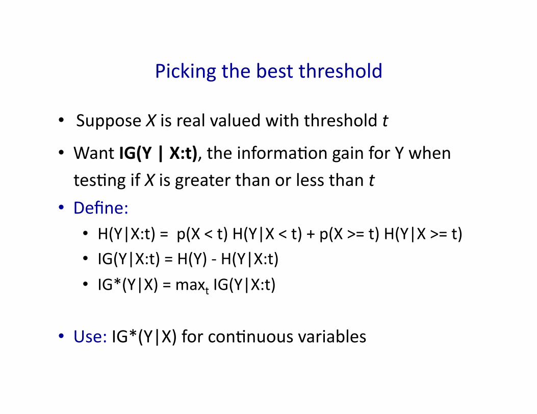
Picking the best threshold

•  Suppose X is real valued with threshold t •  Want IG(Y | X:t), the informaGon gain for Y when tesGng if X is greater than or less than t

•  Define: •  H(Y|X:t) = p(X < t) H(Y|X < t) + p(X >= t) H(Y|X >= t) •  IG(Y|X:t) = H(Y) -‐ H(Y|X:t) •  IG*(Y|X) = maxt IG(Y|X:t)

•  Use: IG*(Y|X) for conGnuous variables

What you need to know about decision trees

•  Decision trees are one of the most popular ML tools –  Easy to understand, implement, and use

–  ComputaGonally cheap (to solve heurisGcally)

•  InformaGon gain to select aIributes (ID3, C4.5,…)

•  Presented for classificaGon, can be used for regression and density esGmaGon too

•  Decision trees will overfit!!! –  Must use tricks to find “simple trees”, e.g.,

•  Fixed depth/Early stopping •  Pruning

– Or, use ensembles of different trees (random forests)

Ensemble learning

Slides adapted from Navneet Goyal, Tan, Steinbach, Kumar, Vibhav Gogate

Ensemble methods

Machine learning competition with a $1 million prize

Bias/Variance Tradeoff

Hastie, Tibshirani, Friedman “Elements of Statistical Learning” 2001

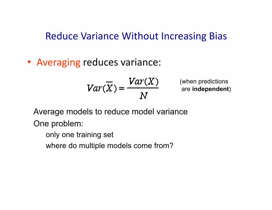
Reduce Variance Without Increasing Bias

•  Averaging reduces variance:

Average models to reduce model variance One problem:

only one training set where do multiple models come from?

(when predictions are independent)

Bagging: Bootstrap AggregaGon

•  Leo Breiman (1994) •  Take repeated bootstrap samples from training set D •  Bootstrap sampling: Given set D containing N training examples, create D’ by drawing N examples at random with replacement from D.

•  Bagging: –  Create k bootstrap samples D1 … Dk. –  Train disGnct classifier on each Di. –  Classify new instance by majority vote / average.

General Idea

Example of Bagging

•  Sampling with replacement

•  Build classifier on each bootstrap sample

•  Each data point has probability (1 – 1/n)n of being selected as test data

•  Training data = 1-‐ (1 – 1/n)n of the original data

Training Data Data ID

51

52

decision tree learning algorithm; very similar to ID3

shades of blue/red indicate strength of vote for particular classification

Random Forests •  Ensemble method specifically designed for decision tree classifiers

•  Introduce two sources of randomness: “Bagging” and “Random input vectors” –  Bagging method: each tree is grown using a bootstrap sample of training data

–  Random vector method: At each node, best split is chosen from a random sample of m aIributes instead of all aIributes

Random Forests

Random Forests Algorithm

Documents

lecture11 - Massachusetts Institute of Technology David&Sontag& New&York&University& Slides adapted from Luke Zettlemoyer, Carlos Guestrin, and Andrew Moore Hypotheses: decision trees