5/22/2009 1

CHAPTER 1. A MATLAB PRIMER

This chapter is based on the Appendix B of the book by Miranda and Fackler and the Getting

Stated Guide of MATLAB. The first important notion is that Matlab works with matrices. A

matrix is a table of numbers with m rows and n columns. A vector is just a particular matrix with

1 row or 1 column.

1. How to create a matrix

1.1. By enumeration

Type

>> X=[1 5;2 1];

The ; at the end of the command means that the result of the command will not appear in the

command window. Next, type

>> X

We get

X =

1 5

2 1

The ; inside the command of the matrix indicates the end of a row.

1.2. By using a MATLAB function

Type

>> X=ones(3,2);X

5/22/2009 2

We get

X =

1 1

1 1

1 1

Or type >> X=zeros(2,3);X

We get

X =

0 0 0

0 0 0

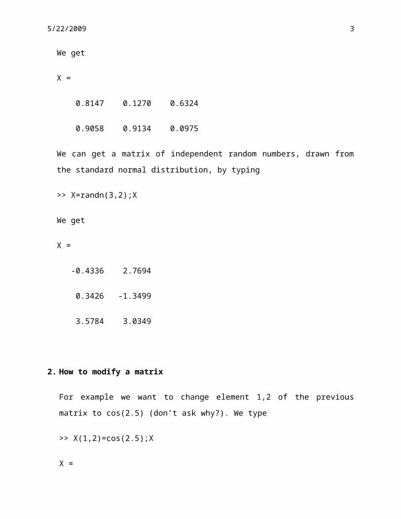
We can get a matrix of independent random numbers, drawn from a uniform distribution by

typing

>> X=rand(2,3);X

We get

X =

0.8147 0.1270 0.6324

0.9058 0.9134 0.0975

We can get a matrix of independent random numbers, drawn from the standard normal

distribution, by typing

>> X=randn(3,2);X

5/22/2009 3

We get

X =

-0.4336 2.7694

0.3426 -1.3499

3.5784 3.0349

2. How to modify a matrix

For example we want to change element 1,2 of the previous matrix to cos(2.5) (don’t ask

why?). We type

>> X(1,2)=cos(2.5);X

X =

-0.4336 -0.8011

0.3426 -1.3499

3.5784 3.0349

We want to set element 2,1 to the same value. We type

>> X(2,1)=X(1,2);X

X =

-0.4336 -0.8011

-0.8011 -1.3499

5/22/2009 4

3.5784 3.0349

We want to set the elements of column 2 to the value log(2). We type

>> X(:,2)=log(2);X

X =

-0.4336 0.6931

-0.8011 0.6931

3.5784 0.6931

Then, we want to set the elements of row 3 to exp(3). We type

>> X(3,:)=exp(3);X

X =

-0.4336 0.6931

-0.8011 0.6931

20.0855 20.0855

Of course, we can type

Y=X(1:2,2);Y

Y =

0.6931

0.6931

5/22/2009 5

3. Matrix algebra

Let us define the two squares matrices A and B (the random –number generator of MATLAB

is very useful for building examples)

>> A=rand(2,2); B=rand(2,2);A,B

A =

0.9572 0.8003

0.4854 0.1419

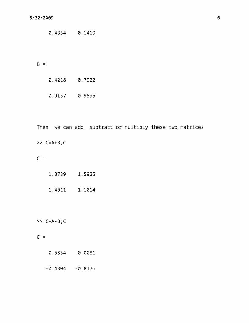
B =

0.4218 0.7922

0.9157 0.9595

Then, we can add, subtract or multiply these two matrices

>> C=A+B;C

C =

1.3789 1.5925

1.4011 1.1014

>> C=A-B;C

5/22/2009 6

C =

0.5354 0.0081

-0.4304 -0.8176

>> C=A*B;C

C =

1.1365 1.5261

0.3346 0.5207

We can also compute the transpose of matrix A, its inverse, its determinant, or put its

diagonal in a vector

>> C=A';C

C =

0.9572 0.4854

0.8003 0.1419

>> C=inv(A);C

C =

-0.5616 3.1678

5/22/2009 7

1.9213 -3.7888

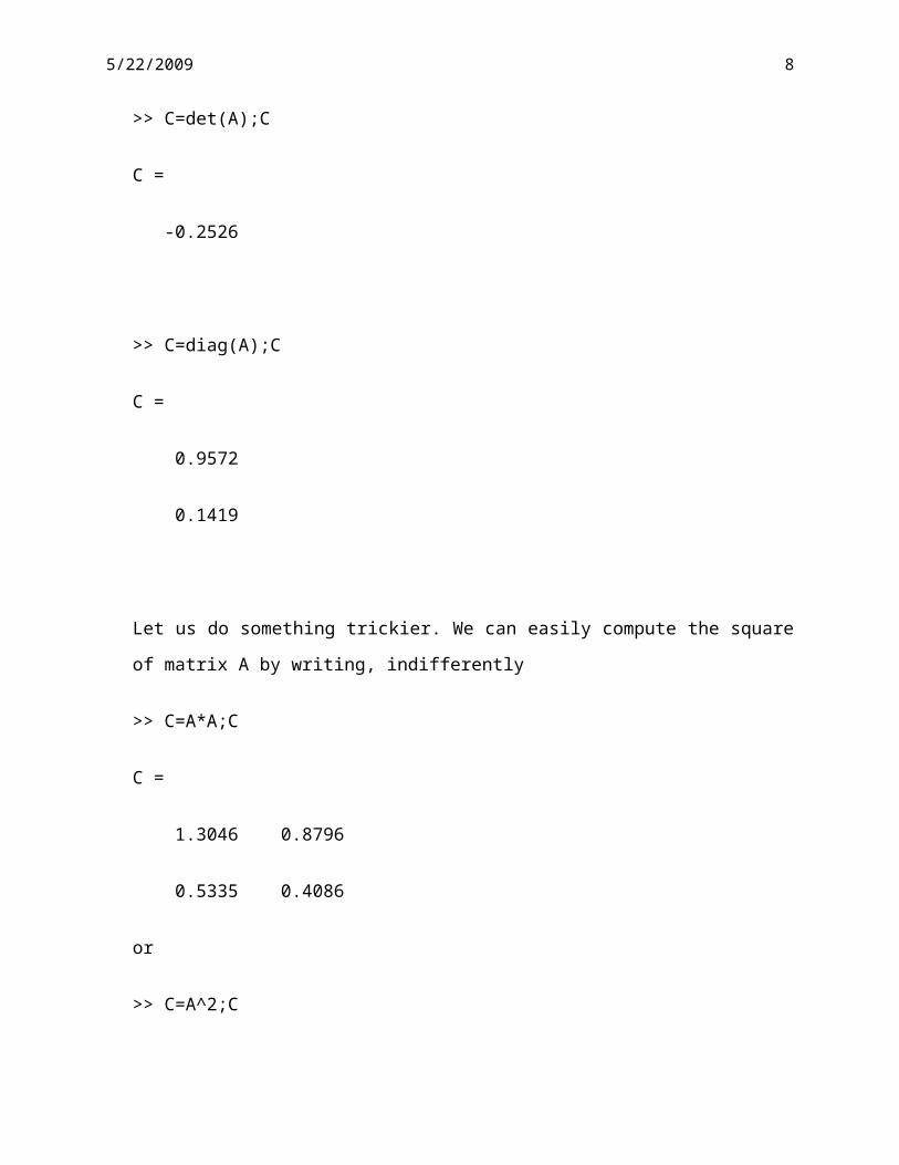
>> C=det(A);C

C =

-0.2526

>> C=diag(A);C

C =

0.9572

0.1419

Let us do something trickier. We can easily compute the square of matrix A by writing,

indifferently

>> C=A*A;C

C =

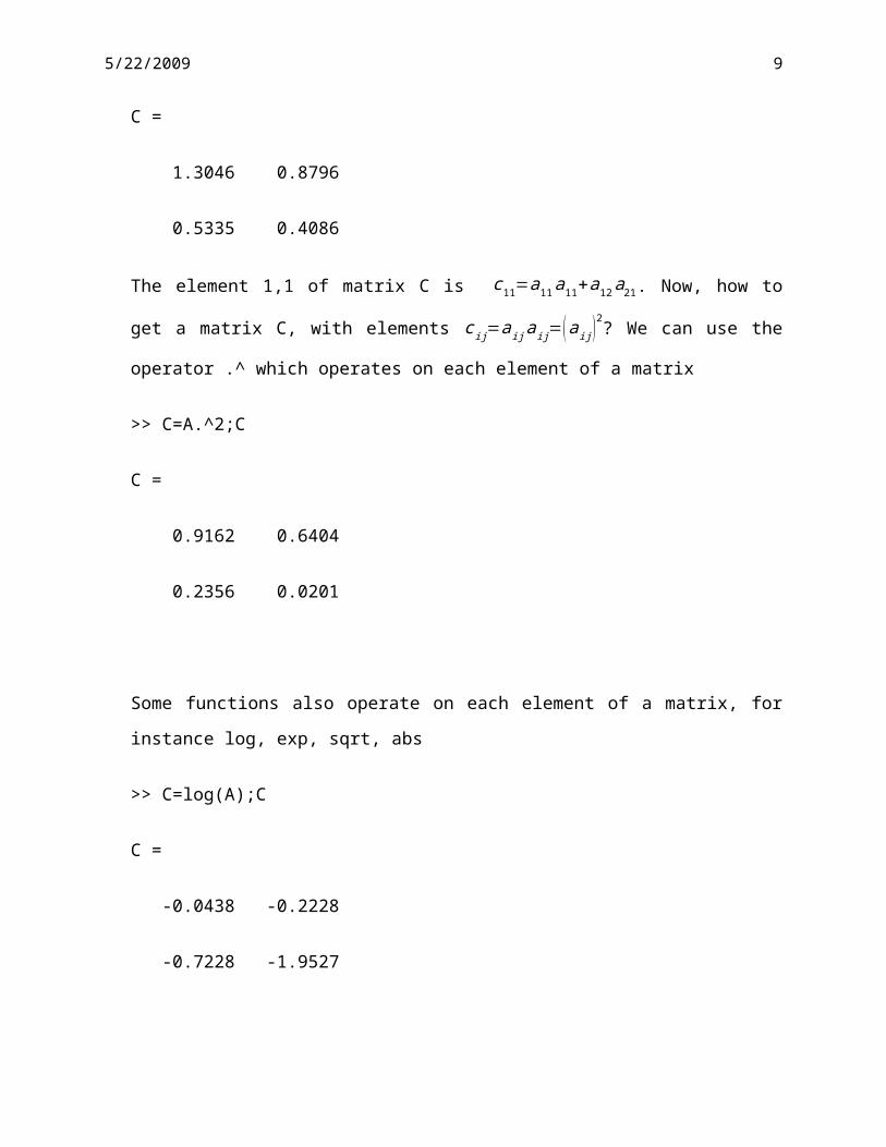
1.3046 0.8796

0.5335 0.4086

or

>> C=A^2;C

5/22/2009 8

C =

1.3046 0.8796

0.5335 0.4086

The element 1,1 of matrix C is c11=a11a11+a12 a21. Now, how to get a matrix C, with

elements c ij=a ij aij=( aij )2? We can use the operator .^ which operates on each element of a

matrix

>> C=A.^2;C

C =

0.9162 0.6404

0.2356 0.0201

Some functions also operate on each element of a matrix, for instance log, exp, sqrt, abs

>> C=log(A);C

C =

-0.0438 -0.2228

-0.7228 -1.9527

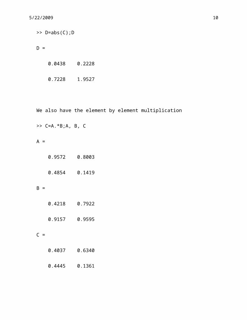
>> D=abs(C);D

D =

5/22/2009 9

0.0438 0.2228

0.7228 1.9527

We also have the element by element multiplication

>> C=A.*B;A, B, C

A =

0.9572 0.8003

0.4854 0.1419

B =

0.4218 0.7922

0.9157 0.9595

C =

0.4037 0.6340

0.4445 0.1361

And the element by element division

>> C=A./B;C

C =

2.2695 1.0102

5/22/2009 10

0.5300 0.1479

4. A few more tricks

If we type >> x=1:1:10;x

We get

x =

1 2 3 4 5 6 7 8 9 10

This command creates a vector of evenly spaced values. The first number in the command is

the starting value of the vector, the second number is the increment and the last number is the

smallest upper bound of the sequence consistent with the starting value and the increment.

If we type >> size(A)

We get

ans =

2 2

If we type >> size(x)

We get

ans =

1 3

5/22/2009 11

The first command gives the dimension of matrix A, and the second command the dimension of

vector x. I did not put a ; at the end of the command lines. So, the results were printed. But as I

did not give a name to the results of the commands, these results were called ans (short for

answer).

5. Conditional statements and looping

5.1. Conditional control

I introduce the two numbers A and B. Then, I write a little program (if I want to write several

lines without executing the program I type … at the end of each of these lines).

>> A=2; B=4;

>> if A > B

'greater'

elseif A < B

'less'

elseif A == B

'equal'

else

error('Unexpected situation')

5/22/2009 12

end

ans =

less

5.2. Loop control

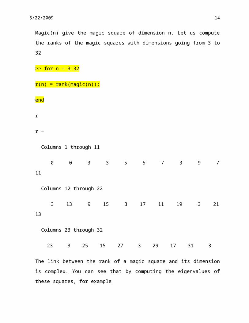
Magic(n) give the magic square of dimension n. Let us compute the ranks of the magic

squares with dimensions going from 3 to 32

>> for n = 3:32

r(n) = rank(magic(n));

end

r

r =

Columns 1 through 11

0 0 3 3 5 5 7 3 9 7 11

Columns 12 through 22

3 13 9 15 3 17 11 19 3 21 13

Columns 23 through 32

23 3 25 15 27 3 29 17 31 3

5/22/2009 13

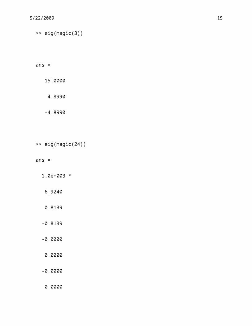
The link between the rank of a magic square and its dimension is complex. You can see that

by computing the eigenvalues of these squares, for example

>> eig(magic(3))

ans =

15.0000

4.8990

-4.8990

>> eig(magic(24))

ans =

1.0e+003 *

6.9240

0.8139

-0.8139

-0.0000

0.0000

-0.0000

0.0000

5/22/2009 14

-0.0000 + 0.0000i

-0.0000 - 0.0000i

-0.0000 + 0.0000i

-0.0000 - 0.0000i

0.0000 + 0.0000i

0.0000 - 0.0000i

0.0000

-0.0000 + 0.0000i

-0.0000 - 0.0000i

-0.0000 + 0.0000i

-0.0000 - 0.0000i

0.0000 + 0.0000i

0.0000 - 0.0000i

0.0000

-0.0000

0.0000 + 0.0000i

0.0000 - 0.0000i

5/22/2009 15

The first eigenvalue is the sum of the magic square (you can check by typing

sum(magic(24))).

The while loop repeats a group of statements an indefinite number of times under control of a

logical condition. A matching end delineates the statements. Here is a complete program,

illustrating while, if, else, and end, that uses interval bisection to find a zero of a polynomial:

>> a = 0; fa = -Inf;

b = 3; fb = Inf;

while b-a > eps*b

x = (a+b)/2;

fx = x^3-2*x-5;

if sign(fx) == sign(fa)

a = x; fa = fx;

else

b = x; fb = fx;

end

end

x

x =

5/22/2009 16

2.0946

Usually you use while for looping when you don’t know how many times the loop is to be

executed and use a for loop when you know how many times it will be executed.

6. Graphics

6.1. Plot

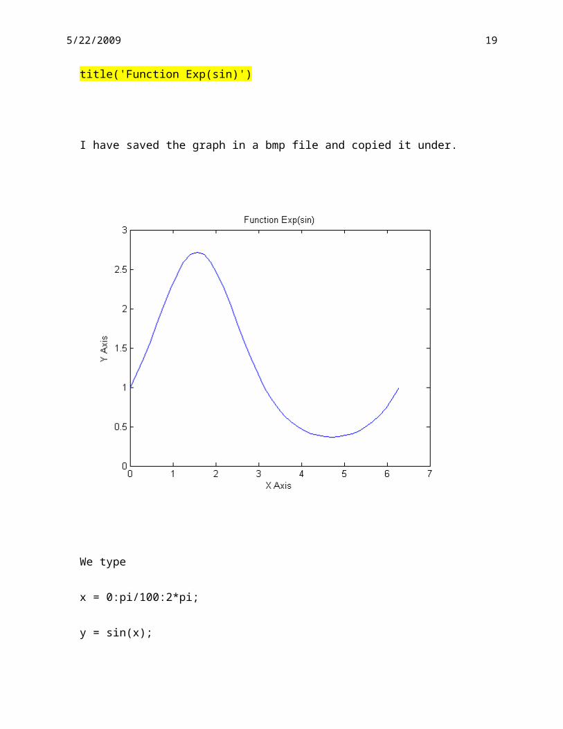
We type

t = 0:pi/20:2*pi;

y = exp(sin(t));

and without interrupting by Enter:

plot(t,y)

xlabel('X Axis')

ylabel('Y Axis')

title('Function Exp(sin)')

I have saved the graph in a bmp file and copied it under.

5/22/2009 17

We type

x = 0:pi/100:2*pi;

y = sin(x);

y2 = sin(x-.25);

y3 = sin(x-.5);

plot(x,y,x,y2,x,y3)

We get

5/22/2009 18

We type

>> [X,Y] = meshgrid(-8:.5:8);

R = sqrt(X.^2 + Y.^2) + eps;

Z = sin(R)./R;

mesh(X,Y,Z)

You can use the round arrow (jut under desktop) to rotate the graph and look for the best

view.

5/22/2009 19

7. Scripts and Functions

Files that contain code in the MATLAB language are called M-files. You create M-files using a

text editor, then use them as you would any other MATLAB function or command. There are

two kinds of M-files:

• Scripts, which do not accept input arguments or return output arguments. They operate on data

in the workspace. If you save a bunch of commands in a script file called MYFILE.m and then

type the word MYFILE at the MATLAB command file, the commands in that file will be

executed just as if you had run them from the MATLAB command prompt. For example, create

a file called magicrank.m that contains these MATLAB commands:

% Investigate the rank of magic squares

r = zeros(1,32);

5/22/2009 20

for n = 3:32

r(n) = rank(magic(n));

end

r

bar(r)

Then, execute the file, either by running it from the debug menu or by typing in the command

window magicrank.

• Functions, which can accept input arguments and return output arguments. Internal variables

are local to the function. Create with the MATLAB editor the file DiagReplace.m (NB.

MATLAB is case sensitive)

function Z = DiagReplace( X,v )

%DiagReplace Put vector v onto diagonal of matrix X

% SYNTAX: Z=DiagReplace(X,v);

n=size(X,1); %return the number of rows of the matrix

Z=X;

ind=(1:n:n*n)+(0:n-1);%The first diagonal element is the first element of the

matrix,

%the second diagonal element is the n+2th element of tye matrix, the third

%diagonal element is the 2*n+3th element of the matrix, etc.

Z(ind)=v;%All the diagonal elements of Z, the position of which was identified

by

%the last command, are substituted by vector v

Then, from the command line type

>> m=3;x=randn(m,m);v=rand(m,1);x,v,xv=DiagReplace(x,v)

You get

x =

-1.0689 1.4384 1.3703

-0.8095 0.3252 -1.7115

5/22/2009 21

-2.9443 -0.7549 -0.1022

v =

0.3816

0.7655

0.7952

xv =

0.3816 1.4384 1.3703

-0.8095 0.7655 -1.7115

-2.9443 -0.7549 0.7952