Embed Size (px)
Citation preview

4/21/2009
1
Package ReliabilityTKK 2009 L 3 P A & B1
James E. MorrisDept of Electrical & Computer Engineering
P l d S U i i
TKK 2009 Lecture 3 Parts A & B1
Portland State University
Package Reliability
A. Reliability TheoryR li bili (b h b ) PDF l i f il f iReliability (bathtub curve), PDF, cumulative failure functionHazard rate, mean time to failureExponential distributionWeibull distributionSystem reliabilityAccelerated testing
4/21/20092
gPlotting failure distributions
B. Package Failure Mechanisms

4/21/2009
2
Potential consequences of poor reliability
Customer Supplier/VendorLoss of Product Warranty claims
Loss of product capability Production downtime
Production downtime Test and repair cost
Spare parts and maintenance Diminished confidence and image
Loss opportunities Loss of future business
4/21/2009 3
Reliability & FailureReliability: The reliability of a product is the probability that the product will perform satisfactorily for a given time at a desired confidence level under specified operating and environmental conditions.Failure is defined as the loss of the ability of the product to perform a required operation in a specific environment.Three types of failure according to when a failure
4/21/20094
Three types of failure according to when a failure occurred during a product’s operating life:
• Infant mortality• “Useful” life• Wear-out failure

4/21/2009
3
The Bathtub CurveIf a plot of the rate failure of a product versus its operating life is constructed from data taken a large sample of identical products placed in operation at t=0
High level stress
Medium stress level
Low stress level
stressRate of failure
4/21/20095
Low stress level
Mission timeInfant mortality
(stress screening)Useful life
(random failures)Wear out
Reliability TheorySample size = Number failed at time =
ont )(tn fNumber failed at time =
Number still operating satisfactorily =
Reliability = and “Unreliability” = Probability device "ok”
t)(tns
osf ntntn =+ )()(
)(tn f
)(tR )(tQ
4/21/20096
Probability device ok)(tR
)(1 /)(1
/)()(
tRntn
ntntQ
os
of
−=−=
=
)(1
/)(1/)(
tQ
ntnntn
of
os
−=
−==

4/21/2009
4
Failure Probability Density Function (PDF)Failure probability function )(tf
)()/1()( tndtdntf fo=
dttdR
dttdQ )()( −==
Cumulative failure function
Similarly and
)()(
)()(0
tFn
tndftQ
o
ft
===∴ ∫ ττ
dt dtdt
∫∞
==t
dfn
tntR s ττ )()()(0
1)(0
=∫∞
ττ df
4/21/2009 7
F(t) here corresponds to the three regions of the bathtub curve
Hazard Rate (“force of mortality”)The Hazard Rate is defined as the number of failures per unit time per number of operational parts left.
tRdtdQtdnt f )]([1)(1)(1)( −
===λ)(tf
=
Note λ(t) = [dnf(t)/dt]/ns ≈ f(t) = [dnf(t)/dt]/n0 if ns ≈ n0i.e. if few failures yet
Cumulative Hazard Rate: )( ln)()( tRttHt
−== ∫λ
dttRdttRdttnt
s )()()()( ===λ )(tR
since R(0)=1Mean Time to Failure (MTTF):
if R(t)→0 for t « ∞.
0∫
4/21/2009 8
∫∞
=0
)(. dttftMTTF ∫∞
⇒0
)( dttR

4/21/2009
5
Function Definition General 2-parameter Weibull (γ=0)
Exponential (η=1, β=1)
Rayleigh (β=2, k=2/η2)
Probability density function
f(t)
kt.exp-½kt2
Reliability relationships, for nf(t) failed and ns(t) surviving at time t of an initial sample of n0.
Survivor function (reliability) R(t)
exp-½kt2
Cumulative failure function (unreliability)
Q(t)=1-R(t)=F(t)
1- 1-1- exp-½kt2
Hazard rate λ(t) kt
4/21/20099
Cumulative hazard rate H(t)
λ0t kt2
Mean time to failure MTTF
1/
Example: Exponential DistributionMost commonly used with wide application in electronic systems. It is a single parameter distribution.
)(exp)( )( tuttf oo
λλ −=
oλ)(tuwhere is the Heavyside step function andis called the chance hazard rate.
)(.exp)( tutf oλ=
∫∞
=t
dftR ττ )()( ]∞∞
−−=−=∫ t0 )exp( ).exp( τλττλλt
oo d )(exp 0tλ−=
and
4/21/2009 10
t t
)(1)( tRtQ −= 1)(0
=∫∞
ττ df

4/21/2009
6
Exponential Distribution
0.80
1.00
1.20Q (t)Q (t)
λ0
f (t)
Area Q (t)
Total Area = 10.00
0.20
0.40
0.60
0 1 2 3 4 5 6
R (t) time t
4/21/200911
0 1 2 3 4 5 6t
Area R (t)ttime
Hazard Rate ("force of mortality")
)()()()(
1
)()(
1)( )0(
tRdt
tdRdt
tdQtR
ndt
tdntn
t f
s
−=⇒
⎯⎯ →⎯= ÷λ
( )0
0
0
0
expexp λλ
λ
λ
=−
−⇒ −
−
t
t
)( dtdttR expfor exponential (Failure frequency at time t)
Mean Time to Failure MTTF∫∞
=0
)(. dttftMTTF0
)(⇒∞
∫ dttR
4/21/200912
00
0
0
1exp1 ] λλ
λ=⎟
⎠⎞
⎜⎝⎛ −=
∞
tfor exponential distribution
i.e. interpret Reliability ⎟⎠⎞
⎜⎝⎛ −
=MTTF
ttR exp)(

4/21/2009
7
Weibull Distribution
β
ηγβ
ηγ
ηβ
⎟⎟⎠
⎞⎜⎜⎝
⎛ −−
−
⎟⎟⎠
⎞⎜⎜⎝
⎛ −=
tttfw exp1
)(
)(tfw is Weibull probability distribution function, where"3-parameter distribution"
ηβγ)(t
exp)(−−
=tR
0=γ "2-parameter Weibull"
101 −λβ e ponential
4/21/200913
,0 , 1 === oληγβ exponential
Weibull Distributionβ > 0 is "shape factor"
0< β< 1 early failureβ =1 constant rateββ >1 wear out
η>0 is "scale factor"
γ is location parameter
4/21/200914
γ pγ < 0 pre-existing failure (storage, transport)γ = 0 failure begins t = 0γ > 0 failure free period t = 0

4/21/2009
8
Weibull Distribution1.4)(tfw
0.2
0.4
0.6
0.8
1
1.2
β=1
β=2
β=3γ=0
η=1
4/21/200915
0
0.2
0 0.5 1 1.5 2
mission time
Effect of shape parameter
Weibull Distribution
)(tf2,0 == βγ
0 80.9
1
)(tfw 1=η
2=η
3η =0 10.20.30.40.50.60.70.8
4/21/200916
t
Effect of scale parameter
00.1
0 0.5 1 1.5 2 2.5mission time

4/21/2009
9
0=γ 2=β 1=η
Weibull Distribution1)(tfw
0<γ0>γ
γ
0.2
0.4
0.6
0.8
4/21/200917Effect of location parameter
-0.2
00 0.5 1 1.5 2 2.5 3
mission time
Weibull Distribution: Hazard Rate(Bathtub Curve)
4
5
β=3
1
2
3
haza
rd r
ate
β=2
β=3/2
β=1
4/21/200918
00 0.5 1 1.5 2 2.5
time
β=1/2
Effects of shape parameter β

4/21/2009
10
Series ReliabilityFailure of a system if any components fails. It is function of the weakest link in the system.
n
n
iss RRRRRR ,..... 321==∏
ssss
n
iss
ni
iss
MTTFλ
λλ
11
3211
=
=∑
∏=
P ll l R li bilit
4/21/200919
Parallel ReliabilityIf there are redundant components
note: for n=2n )1(11
1∏=
−−=−=n
iipsps RQR
ttt
ttt
ps eeeeee)(
)(2121
2121
2121 )(λλλλ
λλλλ λλλλλ +−−−
+−−−
−++−+
=
Effect of series complexity on system reliability
No. ofC
36.60%90.48%99.01%99.90%100
90.44%99.004%99.90%99.99%10
99.00%99.90%99.99%99.999%
System reliability for individual component reliability ofComponentsin series
4/21/2009200.004%36.77%99.48%99.01%1000
0.66%60.64%99.12%99.50%500
8.1%77.87%99531%99.50%250

4/21/2009
11
Accelerated TestingFailure Mechanism (diffusion, corrosion, etc)
kTE /
So, accelerated at higher temperature
kTErr /0
0exp−=
/rα 1 failure totime
4/21/200921
So, Times to failure at , at1t 1T 2t 2T
)11(exp21
0
2
1
TTkE
tt
−= Acceleration factor1/ 21 >tt 21 TT <
Plotting :Weibull Distributionβαexp1)( )/(−= −tQ t ))](1/(1log[log tQ−
αββα β
lnln)](1ln[ln{)/()}(1ln{
exp1)(
−=−−−=−
=
ttQttQ
tQ
or use Cumulative Hazard ratet tlog
slope β
Intercept gives α
4/21/200922
)](ln[)()(0
tRdtttHt
−== ∫λ [ ])(1ln tQ−−=
plot )(log tH vs tlog
tlog
∴

4/21/2009
12
4/21/200923
Plotting: Exponential Distribution
)(1/1 tQ−
ttQ
tH
tQ t
λ
λ
=−
=∴
−= −
)(11ln)(
exp1)( 1000
100
10
1
)(Q
tslope =λ 1−MTTF
4/21/200924
0 100 200 300 4001 t

4/21/2009
13
B. Failure Mechanisms and Modeling1. Mechanical and Thermomechanical Degradation mechanisms
a. Fatigue (Fracture Mechanics) b. Creepc. Stress corrosion cracking
2.Thermo- and Electrotransport Fail Mechanisms. e o d ec o spo ec s sa. Electromigrationb. Thermomigration
3. Electrical and Thermal Degradation Mechanismsa. Dielectric degradation & breakdownb. Contact resistance degradation due to oxidation
4. MIL-HDBK-217 and Physics of Failure5. Chemical and electrochemical failure mechanisms
4/21/200925
a. Corrosionb. Wet and Dry Migration
6. Plastic Package Failuresa. Popcorningb. Dry Packing
7. Distributions of Failures
Plastic Package Failure Mechanisms
4/21/200926

4/21/2009
14
4/21/200927
1. Thermomechanical Deformation in solder joints
4/21/200928

4/21/2009
15
Maximum stress at the edge due to a large DNP(distance from neutral point)
4/21/200929
Nucleation and propagation of fatigue crack in solder joints
4/21/200930

4/21/2009
16
Fatigue life for MCM solder joints on the various substrate materials vs. material's CTE
4/21/200931
Mechanical and Thermo-mechanical Degradation Mechanisms
Mechanical Elastic and plastic deformation
stress
strainε
deformation
σ
4/21/200932
Ideal elastic material

4/21/2009
17
Stress control Strain control
Cyclic dependent hardeningTypical of soft fully annealed
metal samples
ε σ
4/21/200933
Cyclic dependent softening Typical of initially
hard cold worked metal
samples
σε
tcoefficienstrength fatigue'
)2('2
=
=Δ
= NE
f
bff
ea
σ
σεσ
Cyclic Mechanical Testing: Coffin-Manson EquationElasticElastic
exponentstrength failure
failure toreversals load of no. 2
fail tocycles
)"12( reversal load oneat intercept stress"
=
=
=
==
b
N
N
N
f
f
f
f
Pl i
4/21/200934
Plastic
4/21/2009
18
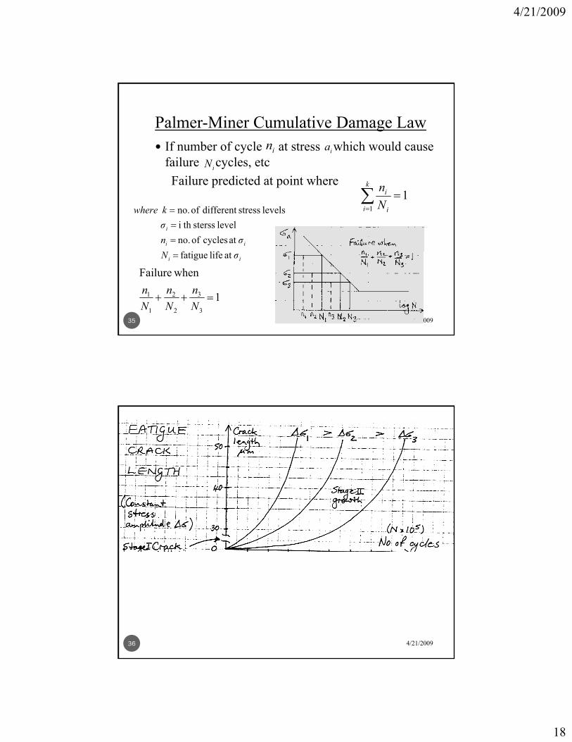
Palmer-Miner Cumulative Damage LawIf number of cycle at stress which would cause failure cycles, etc
iniN
iay ,
Failure predicted at point where1
1=∑
=
k
i i
i
Nn
iN
ii
i
σnσkwhere
liff iat cycles of no.
level sterss th i levels stressdifferent of no.
===
4/21/200935
ii σN at life fatigue =
1
whenFailure
3
3
2
2
1
1 =++Nn
Nn
Nn
4/21/200936


![Publication [IV] - TKK](https://img.pdfslide.us/doc/110x75/61f2fb971a17171fc95f7b67/publication-iv-tkk.jpg)