Embed Size (px)
Citation preview
1
INTRODUCTION TO
Machine LearningETHEM ALPAYDIN© The MIT Press, 2004
Edited for CS 536 Fall 2005 – Rutgers UniversityAhmed Elgammal
This is a draft version. The final version will be posted later
[email protected]://www.cmpe.boun.edu.tr/~ethem/i2ml
Lecture Slides for
CHAPTER 10:
Linear DiscriminationKernel MethodsSupport Vector Machines
2
Lecture Notes for E Alpaydın 2004 Introduction to Machine Learning © The MIT Press (V1.1)3
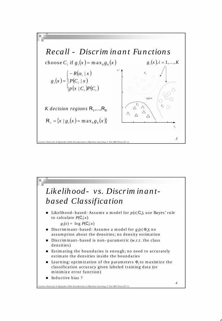
Recall - Discriminant Functions( ) K,,i,gi K1 =x( ) ( )xx kkii ggC maxif choose =
( ) ( ){ }xxx kkii gg max| ==R
K decision regions R1,...,RK
( )( )
( )( ) ( )
−=
ii
i
i
i
CPCpCPR
g||
|
xx
xx
α
Lecture Notes for E Alpaydın 2004 Introduction to Machine Learning © The MIT Press (V1.1)4
Likelihood- vs. Discriminant-based Classification
Likelihood-based: Assume a model for p(x|Ci), use Bayes’ rule to calculate P(Ci|x)
gi(x) = log P(Ci|x)Discriminant-based: Assume a model for gi(x|Φi); no assumption about the densities; no density estimationDiscriminant-based is non-parametric (w.r.t. the class densities)Estimating the boundaries is enough; no need to accurately estimate the densities inside the boundariesLearning: optimization of the parameters Φi to maximize the classification accuracy given labeled training data (or minimize error function)Inductive bias ?
3
Lecture Notes for E Alpaydın 2004 Introduction to Machine Learning © The MIT Press (V1.1)5
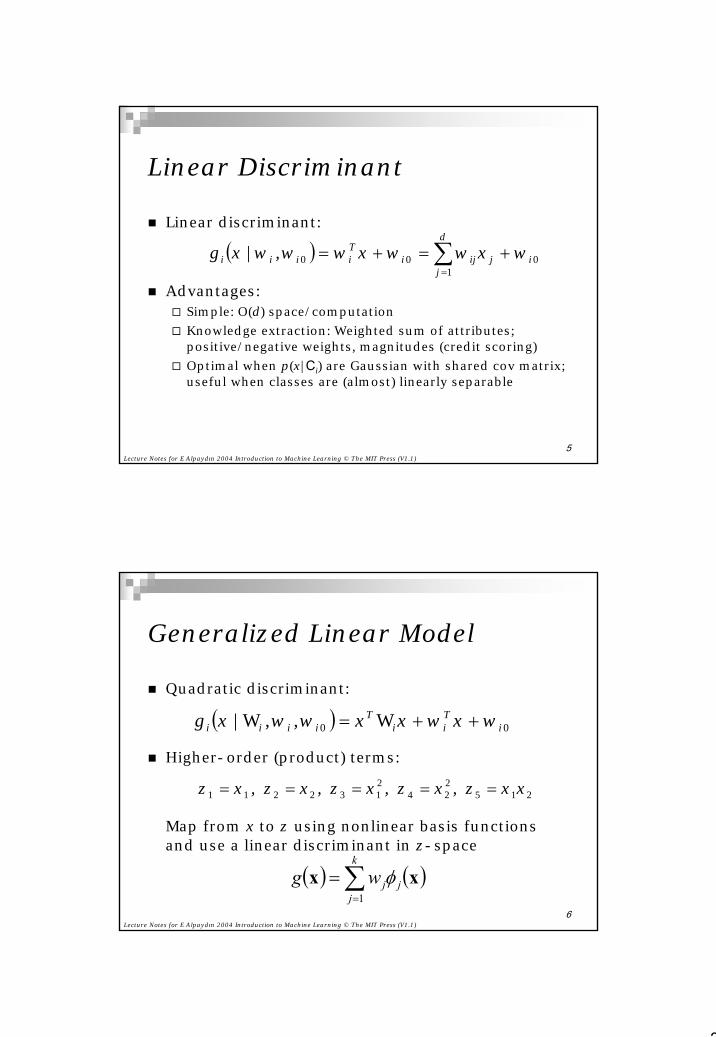
Linear Discriminant
Linear discriminant:
Advantages:Simple: O(d) space/computation Knowledge extraction: Weighted sum of attributes; positive/negative weights, magnitudes (credit scoring)Optimal when p(x|Ci) are Gaussian with shared cov matrix; useful when classes are (almost) linearly separable
( ) 01
00| ij
d
jiji
Tiiii wxwww,g +=+= ∑
=
xwwx
Lecture Notes for E Alpaydın 2004 Introduction to Machine Learning © The MIT Press (V1.1)6
Generalized Linear Model
Quadratic discriminant:
Higher-order (product) terms:
Map from x to z using nonlinear basis functions and use a linear discriminant in z-space
215224
2132211 xxz,xz,xz,xz,xz =====
( ) 00| iTii
Tiiii ww,,g ++= xwxxwx WW
( ) ( )∑=
=k
jjjwg
1
xx φ
4
Lecture Notes for E Alpaydın 2004 Introduction to Machine Learning © The MIT Press (V1.1)7
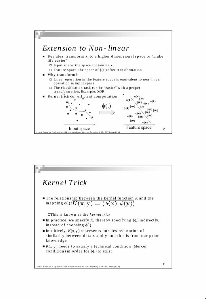
Extension to Non-linearKey idea: transform xi to a higher dimensional space to “make life easier”
Input space: the space containing xiFeature space: the space of φ(xi) after transformation
Why transform?Linear operation in the feature space is equivalent to non-linear operation in input spaceThe classification task can be “easier” with a proper transformation. Example: XOR
Kernel trick for efficient computationφ( )
φ( )
φ( )φ( )φ( )
φ( )
φ( )φ( )
φ(.) φ( )
φ( )
φ( )φ( )φ( )
φ( )
φ( )
φ( )φ( ) φ( )
Feature spaceInput space
Lecture Notes for E Alpaydın 2004 Introduction to Machine Learning © The MIT Press (V1.1)8
Kernel Trick
The relationship between the kernel function K and the mapping φ(.) is
This is known as the kernel trickIn practice, we specify K, thereby specifying φ(.) indirectly, instead of choosing φ(.)Intuitively, K(x,y) represents our desired notion of similarity between data x and y and this is from our prior knowledgeK(x,y) needs to satisfy a technical condition (Mercer condition) in order for φ(.) to exist
5
Lecture Notes for E Alpaydın 2004 Introduction to Machine Learning © The MIT Press (V1.1)9
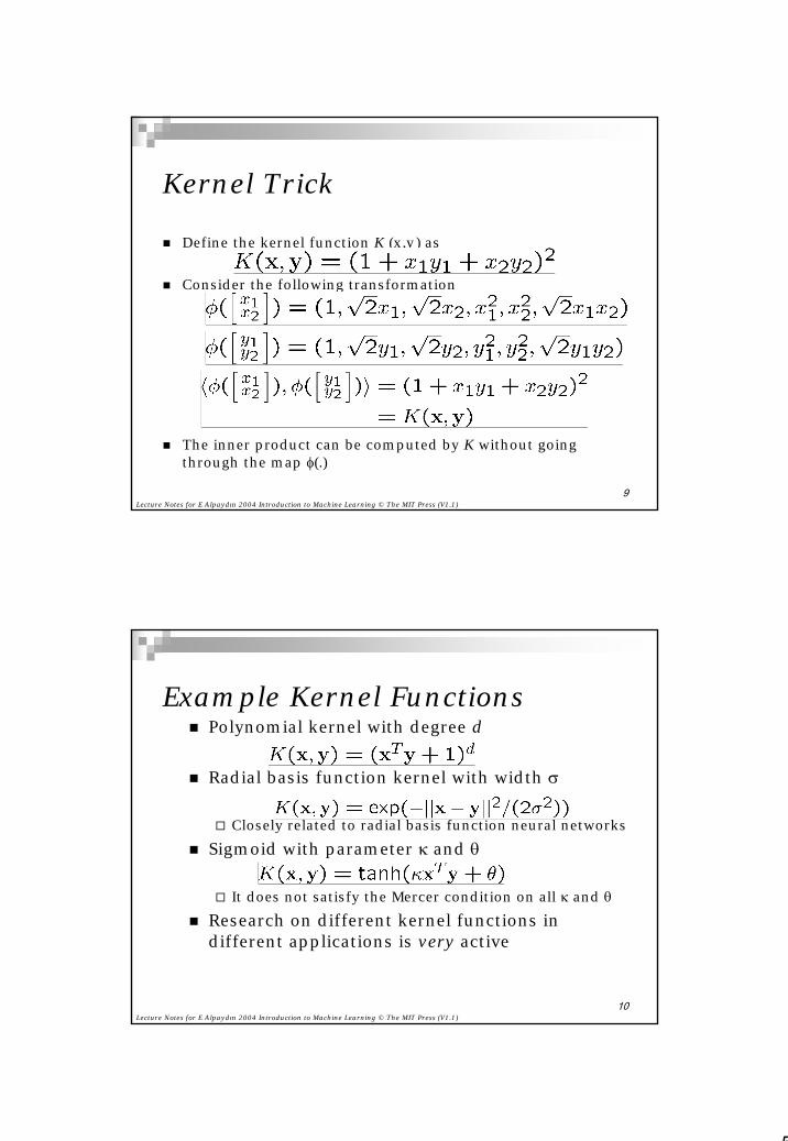
Kernel Trick
Define the kernel function K (x,y) as
Consider the following transformation
The inner product can be computed by K without going through the map φ(.)
Lecture Notes for E Alpaydın 2004 Introduction to Machine Learning © The MIT Press (V1.1)10
Example Kernel FunctionsPolynomial kernel with degree d
Radial basis function kernel with width σ
Closely related to radial basis function neural networksSigmoid with parameter κ and θ
It does not satisfy the Mercer condition on all κ and θResearch on different kernel functions in different applications is very active
6
Lecture Notes for E Alpaydın 2004 Introduction to Machine Learning © The MIT Press (V1.1)11
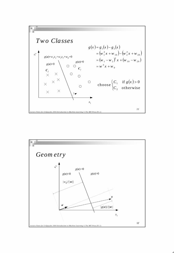
Two Classes( ) ( ) ( )
( ) ( )( ) ( )
0
201021
202101
21
www
wwggg
T
T
TT
+=
−+−=
+−+=
−=
xwxww
xwxwxxx
( ) >
otherwise0if
choose2
1
CgC x
Lecture Notes for E Alpaydın 2004 Introduction to Machine Learning © The MIT Press (V1.1)12
Geometry
7
Lecture Notes for E Alpaydın 2004 Introduction to Machine Learning © The MIT Press (V1.1)13
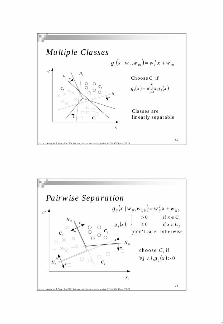
Multiple Classes( ) 00| i
Tiiii ww,g += xwwx
Classes arelinearly separable
( ) ( )xx j
K
ji
i
gg
C
1max
if Choose
==
Lecture Notes for E Alpaydın 2004 Introduction to Machine Learning © The MIT Press (V1.1)14
Pairwise Separation( ) 00| ij
Tijijijij ww,g += xwwx
( )
∈≤∈>
=otherwisecare tdon'if 0if 0
j
i
ij CC
g xx
x
( ) 0if choose>≠∀ xij
i
g,ijC
8
Lecture Notes for E Alpaydın 2004 Introduction to Machine Learning © The MIT Press (V1.1)30
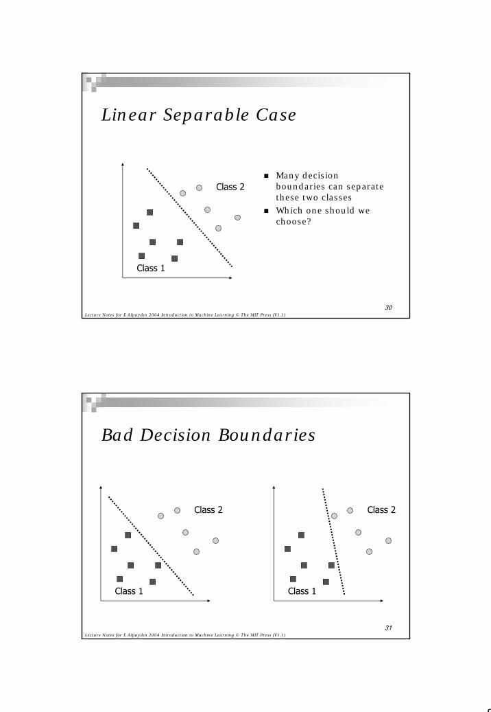
Linear Separable Case
Class 1
Class 2Many decision boundaries can separate these two classesWhich one should we choose?
Lecture Notes for E Alpaydın 2004 Introduction to Machine Learning © The MIT Press (V1.1)31
Bad Decision Boundaries
Class 1
Class 2
Class 1
Class 2
9
Lecture Notes for E Alpaydın 2004 Introduction to Machine Learning © The MIT Press (V1.1)32
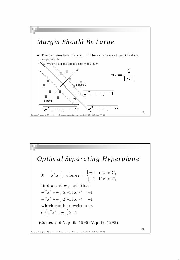
Margin Should Be Large
The decision boundary should be as far away from the data as possible
We should maximize the margin, m
Class 1
Class 2
m
Lecture Notes for E Alpaydın 2004 Introduction to Machine Learning © The MIT Press (V1.1)33
Optimal Separating Hyperplane
(Cortes and Vapnik, 1995; Vapnik, 1995)
{ }
( ) 1as rewritten be can which1 for 11 for 1
that such and findif 1if 1 where
0
0
0
0
2
1
+≥+
−=+≤+
+=+≥+
∈−∈+
==
wr
rwrw
wCCrr,
tTt
ttT
ttT
t
tt
ttt
xw
xwxw
wxxxX
10
Lecture Notes for E Alpaydın 2004 Introduction to Machine Learning © The MIT Press (V1.1)34
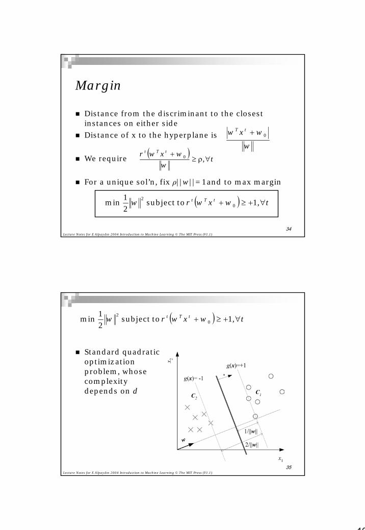
Margin
Distance from the discriminant to the closest instances on either sideDistance of x to the hyperplane is
We require
For a unique sol’n, fix ρ||w||=1and to max margin
wxw 0wtT +
( ) t,wr tTt
∀ρ≥+
wxw 0
( ) t,wr tTt ∀+≥+ 1 to subject 21 min 0
2 xww
Lecture Notes for E Alpaydın 2004 Introduction to Machine Learning © The MIT Press (V1.1)35
( ) t,wr tTt ∀+≥+ 1 to subject 21 min 0
2 xww
Standard quadratic optimization problem, whose complexity depends on d
11
Lecture Notes for E Alpaydın 2004 Introduction to Machine Learning © The MIT Press (V1.1)36
( )
( )[ ]
( )
00
0
21
121
,1 subject to 21 min
10
1
110
2
10
2
02
=⇒=∂∂
=⇒=∂∂
++−=
−+−=
∀+≥+
∑
∑
∑∑
∑
=
=
==
=
N
t
ttp
N
t
tttp
N
t
tN
t
tTtt
N
t
tTttp
tTt
rwL
rL
wr
wrL
twr
α
α
αα
α
xww
xww
xww
xww
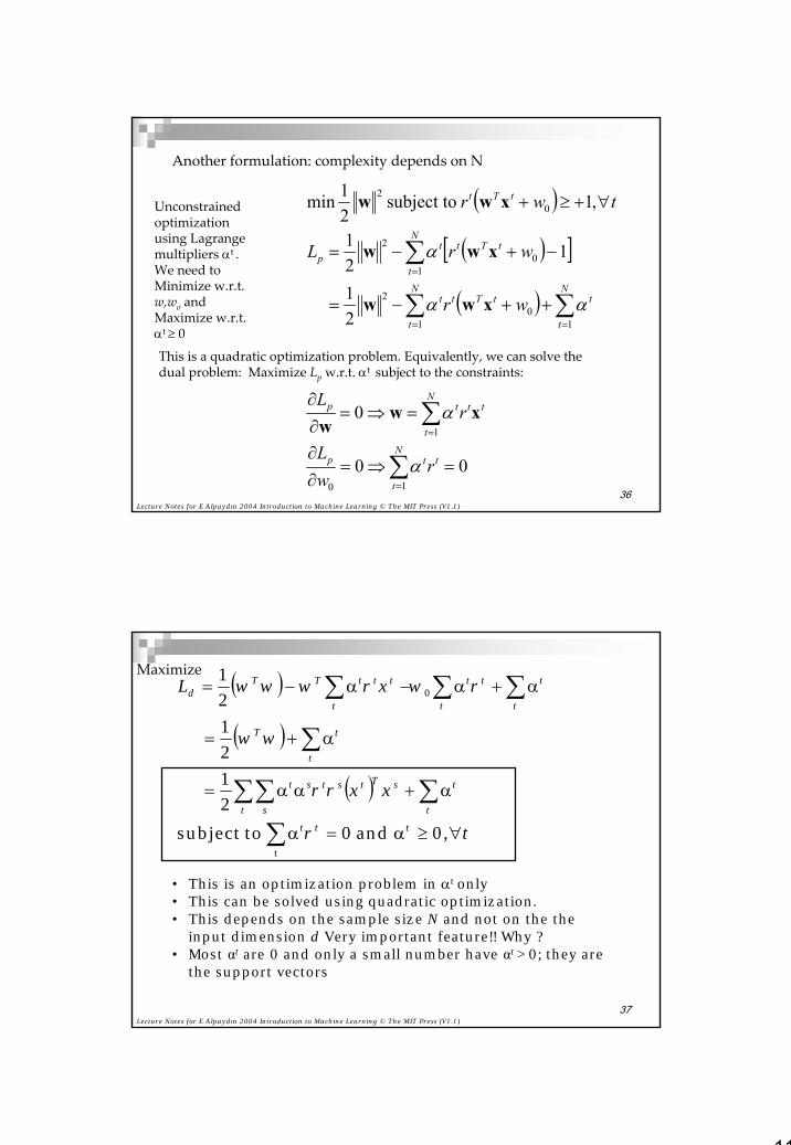
Another formulation: complexity depends on N
Unconstrained optimization using Lagrange multipliers αt .We need to Minimize w.r.t. w,wo andMaximize w.r.t.αt ≥ 0
This is a quadratic optimization problem. Equivalently, we can solve the dual problem: Maximize Lp w.r.t. αt subject to the constraints:
Lecture Notes for E Alpaydın 2004 Introduction to Machine Learning © The MIT Press (V1.1)37
• This is an optimization problem in αt only• This can be solved using quadratic optimization.• This depends on the sample size N and not on the the
input dimension d Very important feature!! Why ?• Most αt are 0 and only a small number have αt >0; they are
the support vectors
( )
( )
( )
∑
∑∑∑
∑
∑ ∑∑
∀≥α=α
α+αα=
α+=
α+α−α−=
t
0
0 and 0 to subject21
21
21
t,r
rr
rwrL
tttt
tsTtst
t s
st
t
tT
t t
ttt
t
tttTTd
xx
ww
xwwwMaximize
12
Lecture Notes for E Alpaydın 2004 Introduction to Machine Learning © The MIT Press (V1.1)38
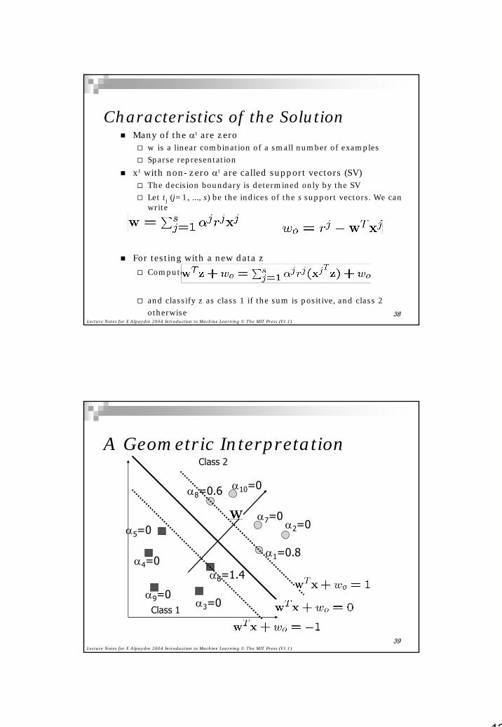
Characteristics of the SolutionMany of the αt are zero
w is a linear combination of a small number of examplesSparse representation
xt with non-zero αt are called support vectors (SV)The decision boundary is determined only by the SVLet tj (j=1, ..., s) be the indices of the s support vectors. We can write
For testing with a new data zCompute
and classify z as class 1 if the sum is positive, and class 2 otherwise
Lecture Notes for E Alpaydın 2004 Introduction to Machine Learning © The MIT Press (V1.1)39
α6=1.4
A Geometric Interpretation
Class 1
Class 2
α1=0.8
α2=0
α3=0
α4=0
α5=0α7=0
α8=0.6
α9=0
α10=0
13
Lecture Notes for E Alpaydın 2004 Introduction to Machine Learning © The MIT Press (V1.1)40
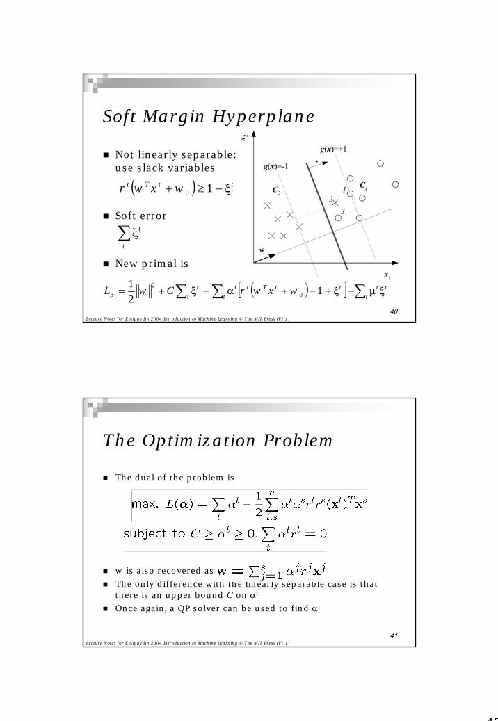
Soft Margin Hyperplane
Not linearly separable: use slack variables
Soft error
New primal is
( ) ttTt wxr ξ−≥+ 10w
∑ξt
t
( )[ ] ∑∑∑ ξµ−ξ+−+α−ξ+=t
ttt
ttTttt
tp wxrCL 1
21
02 ww
Lecture Notes for E Alpaydın 2004 Introduction to Machine Learning © The MIT Press (V1.1)41
The Optimization Problem
The dual of the problem is
w is also recovered asThe only difference with the linearly separable case is that there is an upper bound C on αt
Once again, a QP solver can be used to find αi
14
Lecture Notes for E Alpaydın 2004 Introduction to Machine Learning © The MIT Press (V1.1)42
( )
( ) ( ) ( ) ( )
( ) ( )∑
∑
∑∑
α=
α==
α=α=
t
tttt
TtttT
t
ttt
t
ttt
,Krg
rg
rr
xxx
xφxφxφwx
xφzw
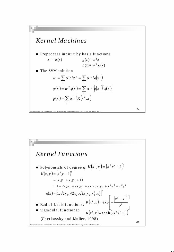
Kernel Machines
Preprocess input x by basis functionsz = φ(x) g(z)=wTz
g(x)=wT φ(x)The SVM solution
Lecture Notes for E Alpaydın 2004 Introduction to Machine Learning © The MIT Press (V1.1)43
Kernel Functions
Polynomials of degree q:
Radial-basis functions:Sigmoidal functions:
( ) ( )qtTt ,K 1+= xxxx
(Cherkassky and Mulier, 1998)
( ) ( )( )
( ) [ ]T
T
x,x,xx,x,x,
yxyxyyxxyxyxyxyx
,K
22
212121
22
22
21
2121212211
22211
2
2221
22211
1
=φ
+++++=
++=
+=
x
yxyx
( )
σ
−−= 2
2
expxx
xxt
t ,K
( ) ( )12tanh += tTt ,K xxxx
15
Lecture Notes for E Alpaydın 2004 Introduction to Machine Learning © The MIT Press (V1.1)44
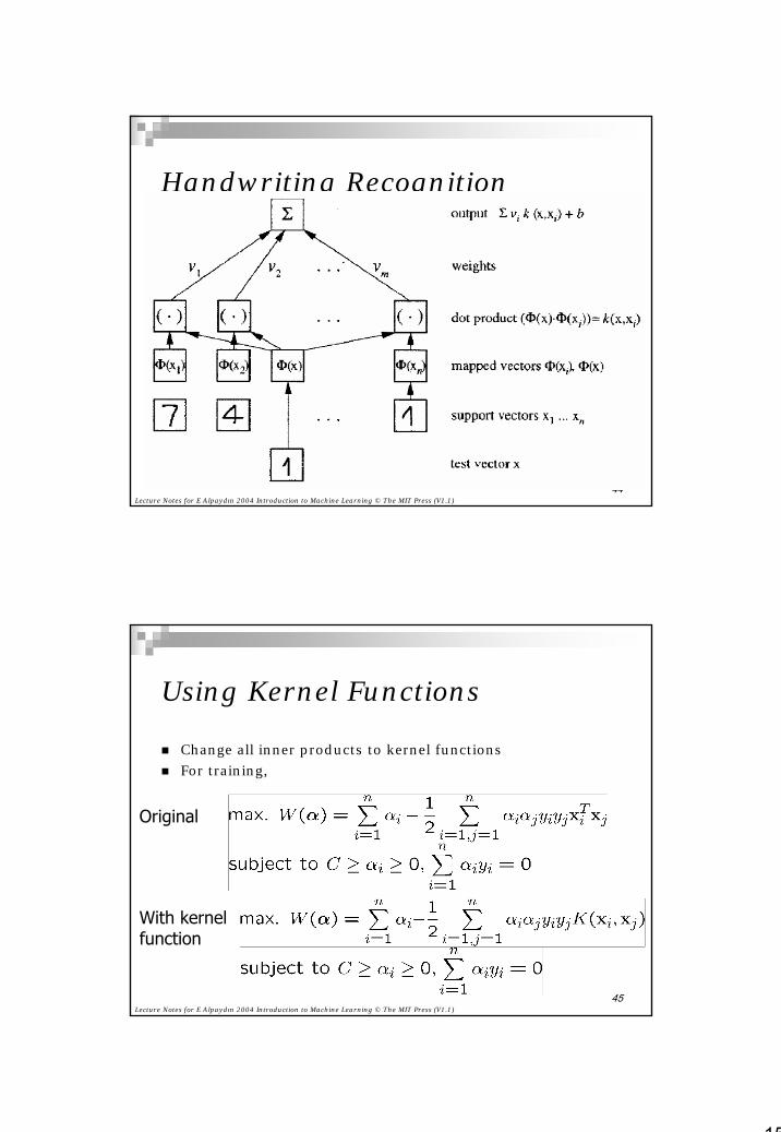
Handwriting Recognition
Lecture Notes for E Alpaydın 2004 Introduction to Machine Learning © The MIT Press (V1.1)45
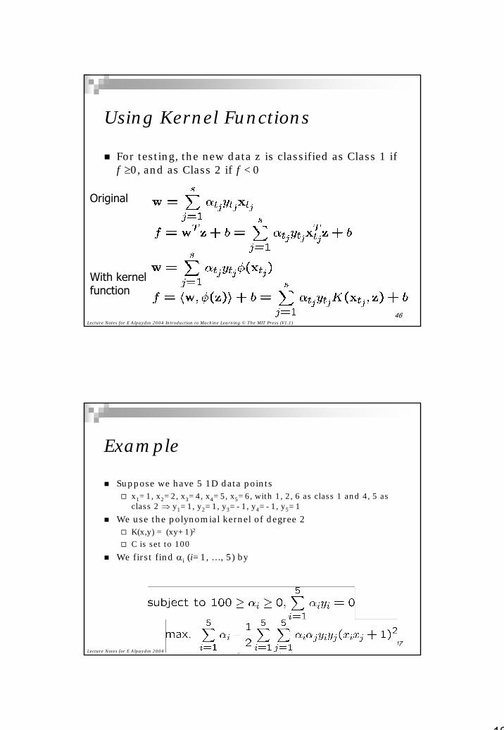
Using Kernel Functions
Change all inner products to kernel functionsFor training,
Original
With kernel function
16
Lecture Notes for E Alpaydın 2004 Introduction to Machine Learning © The MIT Press (V1.1)46
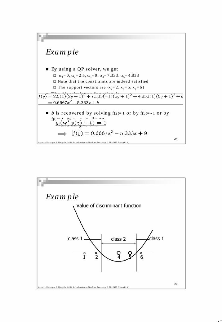
Using Kernel Functions
For testing, the new data z is classified as Class 1 if f ≥0, and as Class 2 if f <0
Original
With kernel function
Lecture Notes for E Alpaydın 2004 Introduction to Machine Learning © The MIT Press (V1.1)47
Example
Suppose we have 5 1D data pointsx1=1, x2=2, x3=4, x4=5, x5=6, with 1, 2, 6 as class 1 and 4, 5 as class 2 ⇒ y1=1, y2=1, y3=-1, y4=-1, y5=1
We use the polynomial kernel of degree 2K(x,y) = (xy+1)2C is set to 100
We first find αi (i=1, …, 5) by
17
Lecture Notes for E Alpaydın 2004 Introduction to Machine Learning © The MIT Press (V1.1)48
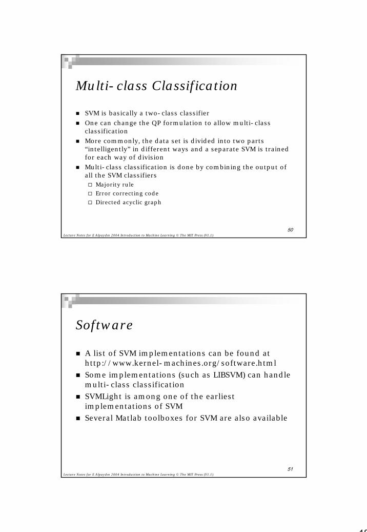
Example
By using a QP solver, we getα1=0, α2=2.5, α3=0, α4=7.333, α5=4.833
Note that the constraints are indeed satisfiedThe support vectors are {x2=2, x4=5, x5=6}
The discriminant function is
b is recovered by solving f(2)=1 or by f(5)=-1 or by f(6)=1, as x2, x4, x5 lie on
and all give b=9
Lecture Notes for E Alpaydın 2004 Introduction to Machine Learning © The MIT Press (V1.1)49
ExampleValue of discriminant function
1 2 4 5 6
class 2 class 1class 1
18
Lecture Notes for E Alpaydın 2004 Introduction to Machine Learning © The MIT Press (V1.1)50
Multi-class Classification
SVM is basically a two-class classifierOne can change the QP formulation to allow multi-class classificationMore commonly, the data set is divided into two parts “intelligently” in different ways and a separate SVM is trained for each way of divisionMulti-class classification is done by combining the output of all the SVM classifiers
Majority ruleError correcting codeDirected acyclic graph
Lecture Notes for E Alpaydın 2004 Introduction to Machine Learning © The MIT Press (V1.1)51
Software
A list of SVM implementations can be found at http://www.kernel-machines.org/software.htmlSome implementations (such as LIBSVM) can handle multi-class classificationSVMLight is among one of the earliest implementations of SVMSeveral Matlab toolboxes for SVM are also available
19
Lecture Notes for E Alpaydın 2004 Introduction to Machine Learning © The MIT Press (V1.1)52
Steps for Classification
Prepare the pattern matrixSelect the kernel function to useSelect the parameter of the kernel function and the value of C
You can use the values suggested by the SVM software, or you can set apart a validation set to determine the values of the parameter
Execute the training algorithm and obtain the αi values Unseen data can be classified using the αi values and the support vectors
Lecture Notes for E Alpaydın 2004 Introduction to Machine Learning © The MIT Press (V1.1)53
SVM Strengths & Weaknesses
StrengthsTraining is relatively easy
No local optimal, unlike in neural networksIt scales relatively well to high dimensional dataTradeoff between classifier complexity and error can be controlled explicitlyNon-traditional data like strings and trees can be used as input to SVM, instead of feature vectors
WeaknessesNeed a “good” kernel function
20
Lecture Notes for E Alpaydın 2004 Introduction to Machine Learning © The MIT Press (V1.1)54
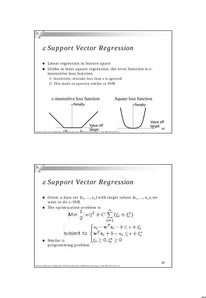
ε Support Vector Regression
Linear regression in feature spaceUnlike in least square regression, the error function is ε-insensitive loss function
Intuitively, mistake less than ε is ignoredThis leads to sparsity similar to SVM
ε−εValue offtarget
Penalty
Value offtarget
Penalty
Square loss functionε-insensitive loss function
Lecture Notes for E Alpaydın 2004 Introduction to Machine Learning © The MIT Press (V1.1)55
ε Support Vector Regression
Given: a data set {x1, ..., xn} with target values {u1, ..., un}, we want to do ε-SVRThe optimization problem is
Similar to SVM, this can be solved as a quadratic programming problem
21
Lecture Notes for E Alpaydın 2004 Introduction to Machine Learning © The MIT Press (V1.1)56
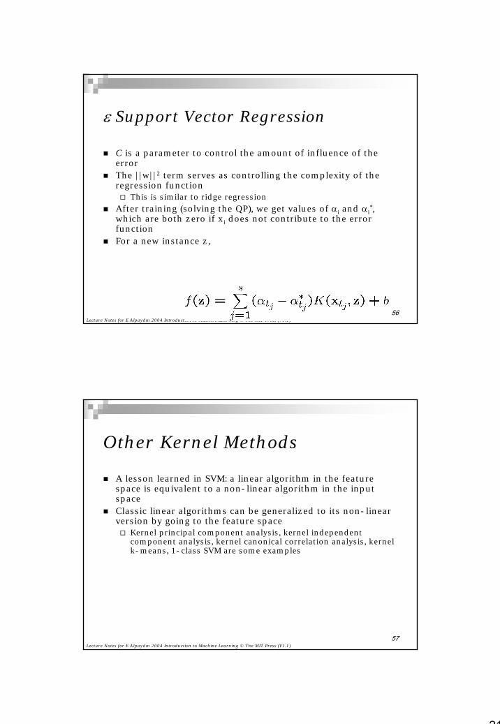
ε Support Vector Regression
C is a parameter to control the amount of influence of the errorThe ||w||2 term serves as controlling the complexity of the regression function
This is similar to ridge regressionAfter training (solving the QP), we get values of αi and αi
*, which are both zero if xi does not contribute to the error functionFor a new instance z,
Lecture Notes for E Alpaydın 2004 Introduction to Machine Learning © The MIT Press (V1.1)57
Other Kernel Methods
A lesson learned in SVM: a linear algorithm in the feature space is equivalent to a non-linear algorithm in the input spaceClassic linear algorithms can be generalized to its non-linear version by going to the feature space
Kernel principal component analysis, kernel independent component analysis, kernel canonical correlation analysis, kernel k-means, 1-class SVM are some examples
22
Lecture Notes for E Alpaydın 2004 Introduction to Machine Learning © The MIT Press (V1.1)58
Conclusion
SVM is a useful method for classificationTwo key concepts of SVM: maximize the margin and the kernel trickMuch active research is taking place on areas related to SVMMany SVM implementations are available on the web for you to try on your data set!
Lecture Notes for E Alpaydın 2004 Introduction to Machine Learning © The MIT Press (V1.1)59
Resources
http://www.kernel-machines.org/http://www.support-vector.net/http://www.support-vector.net/icml-tutorial.pdfhttp://www.kernel-machines.org/papers/tutorial-nips.ps.gzhttp://www.clopinet.com/isabelle/Projects/SVM/applist.html
23
Lecture Notes for E Alpaydın 2004 Introduction to Machine Learning © The MIT Press (V1.1)60
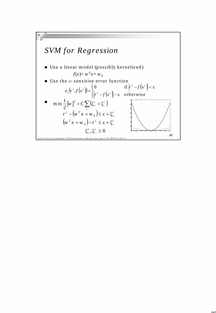
SVM for Regression
Use a linear model (possibly kernelized)f(x)=wTx+w0
Use the є-sensitive error function
( )( ) ( )( )
ε−−
ε<−=ε otherwise
if 0tt
tttt
frfr
f,rex
xx
( )( )
00
0
≥ξξ
ξ+ε≤−+
ξ+ε≤+−
−+
−
+
tt
ttT
tTt
,rw
wrxw
xw
( )∑ −+ ξ+ξ+t
ttC2
21min w