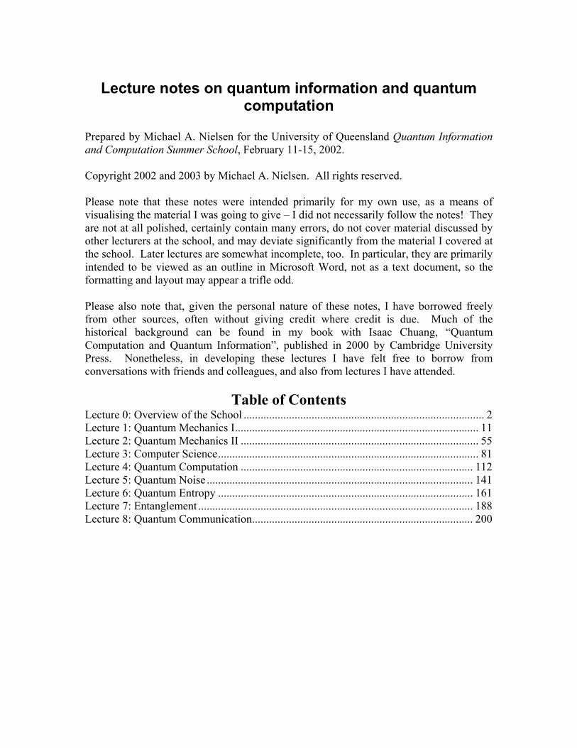
Lecture notes on quantum information and quantum computation

Prepared by Michael A. Nielsen for the University of Queensland Quantum Information and Computation Summer School, February 11-15, 2002. Copyright 2002 and 2003 by Michael A. Nielsen. All rights reserved. Please note that these notes were intended primarily for my own use, as a means of visualising the material I was going to give – I did not necessarily follow the notes! They are not at all polished, certainly contain many errors, do not cover material discussed by other lecturers at the school, and may deviate significantly from the material I covered at the school. Later lectures are somewhat incomplete, too. In particular, they are primarily intended to be viewed as an outline in Microsoft Word, not as a text document, so the formatting and layout may appear a trifle odd. Please also note that, given the personal nature of these notes, I have borrowed freely from other sources, often without giving credit where credit is due. Much of the historical background can be found in my book with Isaac Chuang, “Quantum Computation and Quantum Information”, published in 2000 by Cambridge University Press. Nonetheless, in developing these lectures I have felt free to borrow from conversations with friends and colleagues, and also from lectures I have attended.

Table of Contents

Lecture 0: Overview of the School ..................................................................................... 2 Lecture 1: Quantum Mechanics I...................................................................................... 11 Lecture 2: Quantum Mechanics II .................................................................................... 55 Lecture 3: Computer Science............................................................................................ 81 Lecture 4: Quantum Computation .................................................................................. 112 Lecture 5: Quantum Noise .............................................................................................. 141 Lecture 6: Quantum Entropy .......................................................................................... 161 Lecture 7: Entanglement ................................................................................................. 188 Lecture 8: Quantum Communication.............................................................................. 200

Lecture 0: Overview of the School

Slide: Title

Welcome Welcome, everybody, to the University of Queensland Quantum Information and Computation Summer School.

My own personal feelings about the school I’m very happy that so many of you are here today, and am looking forward to a productive week.

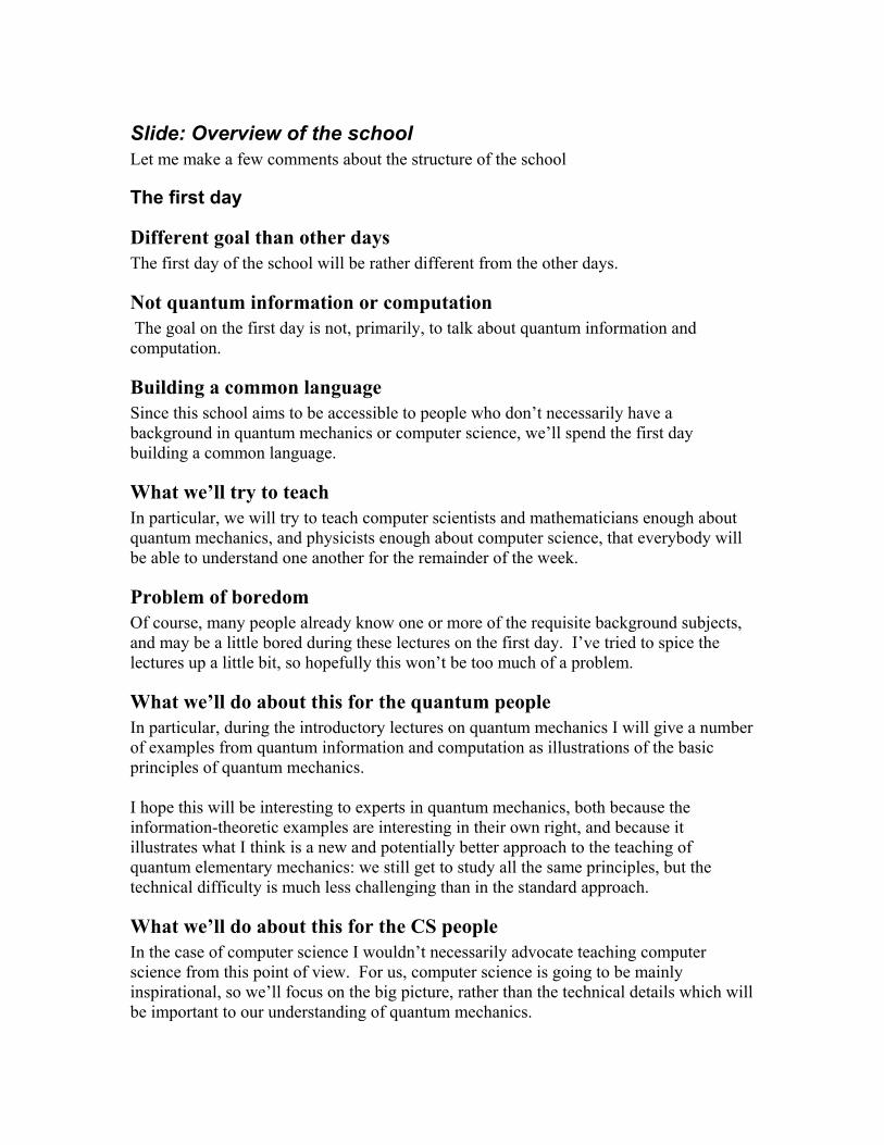
Slide: Overview of the school Let me make a few comments about the structure of the school

The first day

Different goal than other days The first day of the school will be rather different from the other days.

Not quantum information or computation The goal on the first day is not, primarily, to talk about quantum information and computation.

Building a common language Since this school aims to be accessible to people who don’t necessarily have a background in quantum mechanics or computer science, we’ll spend the first day building a common language.

What we’ll try to teach In particular, we will try to teach computer scientists and mathematicians enough about quantum mechanics, and physicists enough about computer science, that everybody will be able to understand one another for the remainder of the week.

Problem of boredom Of course, many people already know one or more of the requisite background subjects, and may be a little bored during these lectures on the first day. I’ve tried to spice the lectures up a little bit, so hopefully this won’t be too much of a problem.

What we’ll do about this for the quantum people In particular, during the introductory lectures on quantum mechanics I will give a number of examples from quantum information and computation as illustrations of the basic principles of quantum mechanics. I hope this will be interesting to experts in quantum mechanics, both because the information-theoretic examples are interesting in their own right, and because it illustrates what I think is a new and potentially better approach to the teaching of quantum elementary mechanics: we still get to study all the same principles, but the technical difficulty is much less challenging than in the standard approach.

What we’ll do about this for the CS people In the case of computer science I wouldn’t necessarily advocate teaching computer science from this point of view. For us, computer science is going to be mainly inspirational, so we’ll focus on the big picture, rather than the technical details which will be important to our understanding of quantum mechanics.

Nonetheless, I hope that even experts in computer science may find there to be something interesting in our rather physically-motivated presentation and revisiting of some of the fundamental ideas of computer science.

Pedagogy through the rest of the week Most of the remainder of the week will be spent on pedagogical lectures covering various aspects of quantum information and computation, as described in more detail in your program.

Tutorials On each of the first three afternoons there will be one hour tutorial sessions, in small groups. During the day’s lectures a number of simple exercises will be posed. You are encouraged to work on those exercises. Then, in the tutorial, you can discuss those problems with the tutor and with other members of the tutorial group, followed by a general question and answer session. Your tutorial group allocation and room location should be found in your summer school pack.

Bob Clark’s lecture One Wednesday evening I’m very pleased to say that Bob Clark will be giving a public lecture about the work on quantum computation in solid-state that is currently being researched by the Centre for Quantum Computer Technology, especially the group at the University of New South Wales.

Research Seminars Finally, on Thursday and Friday afternoon we will have approximately 8 half hour research seminars, designed to give you a feel for some of the research going on in the field.

Slide: Required background Just so we’re all on the same wavelength, let me start out by talking about what background we’ll be assuming. So that we’re all on the same wavelength, let me make a few comments about the background

Restress: don’t need to know quantum mechanics, computer science, or information theory First, let me stress again that you won’t need to know quantum mechanics, computer science or information theory. Please, don’t be concerned if you don’t know all these things, we will attempt to cover the absolute basics of these topics on the first day, and then pick up other material as we go along.

Benefits of a wide variety of backgrounds My personal belief is that quantum information and computation is one of the fields that benefits most from the creative interaction of mathematicians, physicists, computer scientists, and others.

Princeton story Let me tell you a story to illustrate this point. In 1997 I was attending a tutorial workshop at Princeton University. On the first night I had dinner with a friend of mine, and her PhD supervisor. Over dinner, her PhD supervisor confided to me that this week was actually his first week in the field, and that he was a computer scientist who knew almost nothing about quantum mechanics, and was hoping to learn something about quantum mechanics at the workshop. Well, four days later, on the last day of the workshop, I was at a coffee shop, and noticed that this person, the PhD supervisor was busily explaining something to a group of people on a set of napkins. I enquired as to what it was, and it turned out that he had had an idea during the workshop applying his knowledge of computer science to develop a new application of quantum information. That idea has since been written up in a seminal paper about quantum information theory.

The point The point, of course, is not that we are all going to be this lucky. However, I do think it is fair to say that in a field that has just started, like quantum information and computation, there is tremendous scope for people from other fields to leverage their specialist knowledge to gain deep new insights that can greatly enrich the field.

What you do need Having said what you don’t need, I should now say that what you do need is two things. First, you should have a pretty good understanding of elementary linear algebra, vectors, matrices and so forth. We’re going to cover this material again, but we’ll go pretty fast, so today might be a good time to brush up on your linear algebra. Second, you’ll need a fair amount of mathematical maturity. Certainly, beginning postgraduate students in computer science, mathematics and physics should all have the required background. Good third and fourth year undergrads in those disciplines should also be able to cope.

Slide: Philosophy of the school A few words on the philosophy and goals of the school.

Small number of lecturers: unified, coherent, and in-depth, without redundancy First, a relatively small number of lecturers are involved. The intention in doing this is to make the presentation unified, and to eliminate the danger of one lecturer assuming concepts that have not been adequately covered earlier in the week. We’ve worked hard to make sure this does not happen, and I hope that we shall succeed.

Focus on theory rather than implementations Second, the focus of the pedagogical lectures is on fundamental theory, rather than the proposed experimental implementations of that theory. There are several reasons for this. First, it’s a fact that, worldwide, theoretical ideas are currently ahead of experimental implementations, so there are perhaps more theoretical ideas that are of long-lasting value. Second, in Australia experiment is ahead, in the sense that there is a tremendous amount of top-quality experiment going on, but relatively little theoretical work. One of the goals of the summer school, therefore, is to stimulate work, both theoretical and experimental, but especially research work on the theoretical side. To that end a number of open problems in theory will be posed during the school, in the hope that it will stimulate researchers in theory. Third, there are, in fact, too many experimental proposals to really do justice in the limited time we have available. Describing even one of these proposals in details would require several days. Rather than do this, the approach we are going to take is for there to be a general pedagogical talk on the fundamental principles underlying experimental implementations, given by Andrew White, tomorrow. Then, during the research seminars, some of my experimental colleagues will give an overview of the experimental work that is being done in Australia.

Research Networks Another aim of the school is to bring together people with a common interest in quantum information and computation. To that end, at the end of this week we will put all the names and email addresses of people attending the school up on the school web page. Please let us know if you would prefer this not to occur.

Goal of the school Finally, the general aim of the school is to bring you, the audience, up to the cutting edge of research in some aspects of quantum information and computation, and to make it easier to get to that cutting edge in other aspects of the field.

Slide: Miscellany Notes on this viewgraph to be added.

Slide: People involved

Who’s who at the school Let me conclude this introduction by pointing out to you some of the people involved in the school. If you’re having difficulties and need help, these are the people to go to for assistance.

Me You are, of course, always welcome to come to me for assistance.

The organizing committee You should also feel free to contact members of the organizing committee. (Introduce those people by name).

The tutors For many inquiries, it is likely best to start by talking to one of the tutors. (Introduce those people by name.)

The speakers Finally, let me mention also the speaker’s names. I won’t introduce all those people now, as you will see them later in the week.

Lecture 1: Quantum Mechanics I

Slide: Title

What these first two lectures do The goal of this and the next lecture is to introduce _all_ the basic elements of quantum mechanics, using examples drawn from quantum information science.

The umbrella term “quantum information science” Notice, by the way, my use of the umbrella term “quantum information science”. Over the next few days, I’ll continue to use this term as a catch-all for all aspects of quantum information and quantum computation.

Usual, fearsome image Quantum mechanics has a fearsome popular image. Huge, two-volume works on the subject are written. Yet I’m telling you that we can learn quantum mechanics in a couple of days.

Why this is the case My belief is that the reason for this fearsome reputation and the enormous tomes is that the mathematics required to apply quantum mechanics to traditional problems like determining the spectra of molecules and calculating scattering cross-sections is extremely forbidding.

Contrast with quantum information science By contrast, the mathematics used in applications to quantum information science is quite simple. Thus, quantum information science provides a wonderful laboratory for the understanding of all the basic principles of quantum mechanics in a simple and relatively painless way, without the technical difficulties involved in more traditional applications like those studied in traditional texts.

Advantage: don’t need to read those texts A major advantage, of course, is that when you’re just getting into the field, you don’t need to wade through 1500 pages texts, like this one.

Slide: What is quantum mechanics?

Opening question Let me begin by answering, in broad terms, the question “what is quantum mechanics?”

Strategy: clear up a misconception I will begin my explanation by attempting to clear up what I think is a common misconception about quantum mechanics.

Explain the misconception That misconception is that quantum mechanics is a complete physical theory of the world.

State my belief that this is wrong It is not.

Explain how quantum mechanics should really be viewed Quantum mechanics is merely a framework for the development of physical theories, it is not a complete physical theory in its own right.

Analogy of the operating system and applications software

Explain the analogous situation An analogous situation occurs in computing, where useful software consists of two parts, the operating system, which is common to all software, and which sets up a basic framework for doing things like input and output, and the applications software, which builds on the operating system to accomplish useful tasks.

Explain how it works in quantum mechanics In a similar way, the laws of quantum mechanics set up a basic framework for the construction of physical theories, but in any given instance they don’t tell you what those rules are. Those have to be added in.

Example of electrons and photons Let me give you an example. The rules of quantum mechanics don’t tell us how electrons should interact with photons, the particles of light. Indeed, the rules of quantum mechanics don’t even tell us that things like electrons or photons should exist. However, the best theory we have describing the interaction of electrons and photons, called quantum electrodynamics, consists of a set of rules, all phrased within the rules of quantum mechanics, and telling us how electrons and photons should be described, and how they interact.

What quantum mechanics is

Change of topic I’ve told you what quantum mechanics is not. Now let me tell you what it is.

Assertion: it’s a set of four mathematical postulates It is, simply, a set of four mathematical postulates. That’s all it is – four surprisingly simple postulates which lay the ground rules for our description of the world.

My goal in the next two lectures My goal in the next two lectures is to explain those postulates to you, and to work through enough examples of those postulates in action that you’ll be able to apply them independently.

Conclusion of the slide

How I intend to conclude the slide: re-emphasizing this fundamental point about quantum mechanics Let me conclude this slide with another analogy to emphasize the point that quantum mechanics is not a complete physical theory in its own right, but rather needs additional rules to obtain a complete physical theory.

Newtonian mechanics analogy The analogy is to Newtonian mechanics, as you have all seen in your high-school physics courses.

The basic rules; they don’t specify a complete physical theory Newton’s three laws of motion set up a framework governing the laws of physics. However, they don’t determine how two bodies will interact in any given situation.

Need for laws of force For that, we need additional laws like Newton’s law of universal gravitation, describing how massive bodies interact.

Comparison to quantum mechanics The analogy with quantum mechanics is particularly good in this case: quantum mechanics plays a role analogous to Newton’s laws of motion, but there is still the need for additional laws to determine how physical systems will actually behave.

Slide: How successful is quantum mechanics?

Raise the question: How successful is quantum mechanics? How successful is quantum mechanics?

Answer the question! The answer is that it is simply unbelievably successful.

Describe the range of phenomena described by quantum mechanics People often misleadingly describe quantum mechanics as being just about the microscopic world, but in fact quantum mechanics forms the basis for our description of an absolutely remarkable range of phenomena, including things like how stars shine, how the Universe formed, and why matter, including the chairs you’re sitting on, is stable.

The fact that no deviations have been found No deviations from quantum mechanics have ever been found.

Note how hard people have tried to find deviations I should note, by the way, that it is now 80 or so years since the original formulation of quantum mechanics, and an incredible number of people have tried very hard to find a deviation from quantum mechanics. Finding such a deviation will mean a certain Nobel prize and scientific immortality. Nobody has ever found one, despite all this effort.

Belief that a theory of everything will be quantum mechanical Because of this spectacular success, most physicists believe that a so-called “theory of everything”, should one ever be found, will be an essentially quantum-mechanical theory – that is, it will be a theory built within the framework of quantum mechanics.

Question: are there any failures for qm? Given all this stunning success, are there any clouds darkening the horizon for quantum mechanics?

Two clouds on the horizon I would be remiss if I did not mention two clouds that are there, and which have been known since the earliest days of quantum mechanics.

First cloud: the measurement problem The first of these clouds is a conceptual issue related to the basic principles of quantum mechanics, often known as the “measurement problem”. I will describe the measurement problem later in this lecture.

Second cloud: failure to unify gravitation and quantum mechanics The second cloud is that, so far, gravitation has resisted all attempts to be incorporated into the framework of quantum mechanics. All the other fundamental forces of nature

can be described within the quantum mechanical framework, but nobody has yet succeeded in doing so with gravitation.

Slide: The structure of quantum mechanics Having said a little about what quantum mechanics is and isn’t, let me now give an overview of the main components of quantum mechanics.

Three basic elements There are three basic elements you need to master in order to learn quantum mechanics.

First element: linear algebra The first of these elements is elementary linear algebra. Quantum mechanics is phrased in terms of concepts like vectors, matrices, and inner products, which come from linear algebra. The best preparation you can have for doing quantum mechanics is a strong background in linear algebra.

This background is assumed I will mostly assume that you have you such a background in what follows, although I will give you reminders about the basic definitions.

Second element: the Dirac notation The second element is a notation known by physicists as the Dirac notation.

The appearance of the Dirac notation If you don’t know quantum mechanics, and see the Dirac notation in a paper or a book, you could be forgiven for finding it rather forbidding. It certainly appears rather strange and complicated.

The reality of the Dirac notation This is unfortunate, for the Dirac notation is really a very simple notation used by physicists for the notions of linear algebra, such as vectors and matrices.

Natural question: why introduce the notation? Now, you might wonder why physicists go to the trouble of introducing all this strange notation for linear algebraic concepts, when you’ve already learnt a perfectly good notation for it from mathematicians in your undergraduate classes.

Good point, and how we’re going to deal with it This is, I must admit, a good question. However, the fact of the matter is that pretty much all people working in quantum information science use this notation, so we’d better master it too. I’m going to spend quite a bit of time today explaining this notation, and giving some detailed examples to help you get comfortable.

How the audience should deal with it

However, if you haven’t seen the notation before, I highly recommend that you work through some examples on your own. Later in the week you’ll need to find using the Dirac notation as easy as breathing in order to follow those arguments.

Third element: the postulates of quantum mechanics The third and most important element that we need to master is the four basic postulates of quantum mechanics.

Connect to the notion of quantum mechanics as a mathematical framework I said that quantum mechanics is a mathematical framework for the construction of detailed physical theories. In fact, all it contains is four postulates which set the framework for the construction of other physical theories.

Example of QED We say that a theory like quantum electrodynamics is “quantum mechanical” precisely because it fits into this framework of four postulates.

Simplicity of the postulates It may surprise you to learn that each of the four postulates is actually quite simple.

Form of the postulates Indeed, the basic form of each postulate is the same. Namely, each postulate takes a physical concept, and asserts that the correct way to describe that concept is in terms of some mathematical concept. It just so happens that the mathematical concepts used are all drawn from linear algebra, which is why having a good mastery of linear algebra is so important to the study of quantum mechanics.

Overview To illustrate these ideas, let me quickly give you an overview of what each of the four postulates says. I’m just going to run quickly through these; rather than looking at the details now, you should be trying to get a feel for the overall form. I’m also going to give you a list of buzzwords to watch for later – these are important.

Postulate 1: states Postulate 1 is all about how we describea quantum system.

Analogy to weather In most areas of science there is some standard way of describing systems. In meteorology, for example, we use temperature, pressure, and humidity to describe the state of the atmosphere. In quantum mechanics postulate one prescribes for us what the analogous way of describing the state of a quantum system is.

Postulate 2: dynamics The second postulate is all about the allowed dynamics, or time evolution, that may occur in a quantum system. It turns out that not just any dynamics can occur; we can’t have quantum states moving arbitrarily to other quantum states. Instead, there is a so-called “unitarity” restriction placed on the dynamics.

Postulate 3: measurement The third postulate is a little unusual. In most areas of science we’re used to being able to determine the state of a system without too much difficulty.

Example For example, in meteorology, you can just go and measure the temperature, pressure and humidity.

The situation in quantum mechanics The situation in quantum mechanics is rather different. It turns out to be impossible to determine the quantum state of a system directly. Instead, a restricted amount of information can be read out from a quantum system system. The third postulate prescribes exactly what types of information can be read out by measurement.

Postulate 4: composite systems The first postulate told us how to describe the state of a quantum system. The fourth postulate provides a way of relating the state of a composite of two or more quantum systems to the states of the individual systems.

What I’m now going to do Over the next few viewgraphs I’m going to explain each of these postulates in detail, and give some examples. My second lecture today will be almost entirely simple examples of these postulates in action, designed to make you feel comfortable.

Fact that this is all there is to quantum mechanics It may surprise you to learn that this is all there is to quantum mechanics. There’s nothing more to learn, and most of the remainder of this week will be spent working out consequences of these postulates.

Slide: qubits

What I’m going to describe on this viewgraph Postulate 1 is all about how we describe the state of quantum systems. So I’m going to start of my explanation of postulate one by telling you now how we describe the state of the simplest possible quantum system.

Disclaimer on the difficulty of understanding Don’t be worried if the description I’m about to give you seems rather strange. Quite the converse. If you don’t find this description strange then it’s probably a good idea to worry.

History Quantum mechanics took twenty-five years to develop from its initial form to the form in which it is used today, and many of the world’s finest minds struggled with the problem of finding the right formulation of the postulates. In the final years of the struggle, one of the main contributors, Wolfgang Pauli, wrote to a friend that he was finding physics far too difficult at that time, and wished that he had a job as an entertainer, instead.

Status today Even today, eighty or so years later, there is nobody in the world who can really claim to have a good intuitive understanding of these postulates.

How to approach this The way to approach this is to open your mind, simply accept these postulates at face value, and then to begin exploring consequences of the postulates, trying to develop a good feel for them.

What that simple system is: the “qubit” The simplest possible quantum system is known as the “qubit”, which is short for “quantum bit”. Physicists would call this system a “two-level quantum system”, although I’m not going to use that terminology much.

How does this connect to physics? Many of you are probably wondering what on earth a qubit is, physically. If you walk into a lab, you’ll hear people talking about electrons, about photons, and about other particles. But you won’t usually hear them talking about the qubits they find in their labs.

The reason for this The reason for this is that the qubit is not actually a physical system at all. Instead, a qubit is an idealization, a type of model system. According to the rules of quantum mechanics, it is the simplest possible type of physical system.

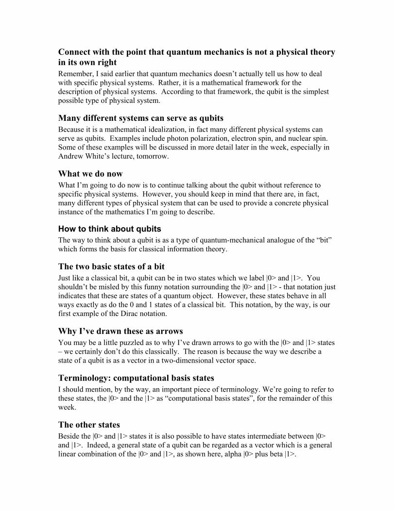
Connect with the point that quantum mechanics is not a physical theory in its own right Remember, I said earlier that quantum mechanics doesn’t actually tell us how to deal with specific physical systems. Rather, it is a mathematical framework for the description of physical systems. According to that framework, the qubit is the simplest possible type of physical system.

Many different systems can serve as qubits Because it is a mathematical idealization, in fact many different physical systems can serve as qubits. Examples include photon polarization, electron spin, and nuclear spin. Some of these examples will be discussed in more detail later in the week, especially in Andrew White’s lecture, tomorrow.

What we do now What I’m going to do now is to continue talking about the qubit without reference to specific physical systems. However, you should keep in mind that there are, in fact, many different types of physical system that can be used to provide a concrete physical instance of the mathematics I’m going to describe.

How to think about qubits The way to think about a qubit is as a type of quantum-mechanical analogue of the “bit” which forms the basis for classical information theory.

The two basic states of a bit Just like a classical bit, a qubit can be in two states which we label |0> and |1>. You shouldn’t be misled by this funny notation surrounding the |0> and |1> - that notation just indicates that these are states of a quantum object. However, these states behave in all ways exactly as do the 0 and 1 states of a classical bit. This notation, by the way, is our first example of the Dirac notation.

Why I’ve drawn these as arrows You may be a little puzzled as to why I’ve drawn arrows to go with the |0> and |1> states – we certainly don’t do this classically. The reason is because the way we describe a state of a qubit is as a vector in a two-dimensional vector space.

Terminology: computational basis states I should mention, by the way, an important piece of terminology. We’re going to refer to these states, the |0> and the |1> as “computational basis states”, for the remainder of this week.

The other states Beside the |0> and |1> states it is also possible to have states intermediate between |0> and |1>. Indeed, a general state of a qubit can be regarded as a vector which is a general linear combination of the |0> and |1>, as shown here, alpha |0> plus beta |1>.

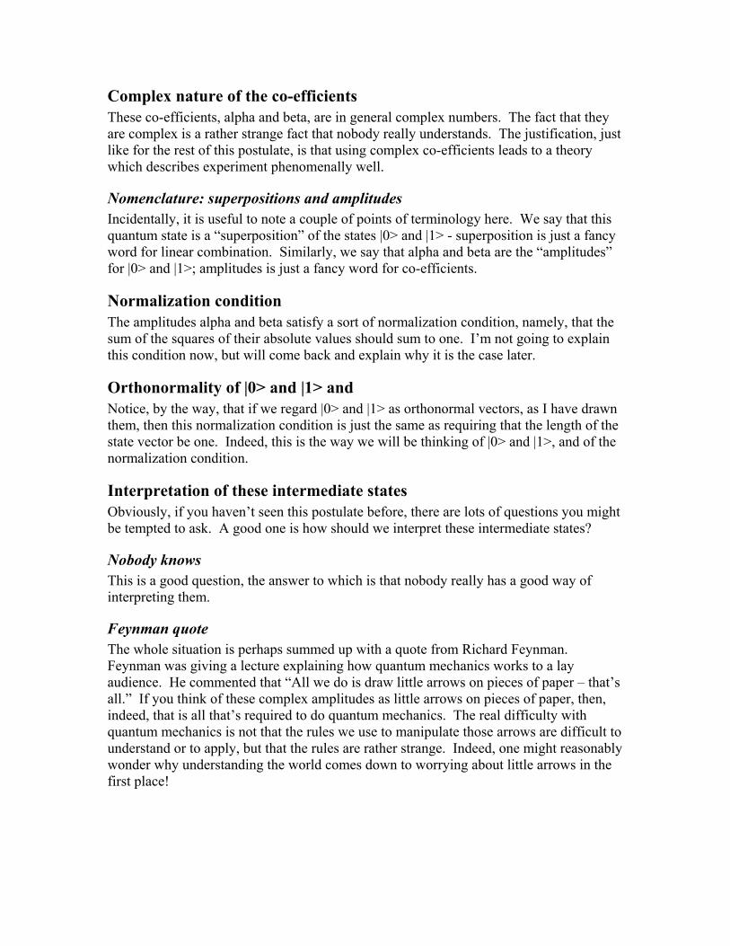
Complex nature of the co-efficients These co-efficients, alpha and beta, are in general complex numbers. The fact that they are complex is a rather strange fact that nobody really understands. The justification, just like for the rest of this postulate, is that using complex co-efficients leads to a theory which describes experiment phenomenally well.

Nomenclature: superpositions and amplitudes Incidentally, it is useful to note a couple of points of terminology here. We say that this quantum state is a “superposition” of the states |0> and |1> - superposition is just a fancy word for linear combination. Similarly, we say that alpha and beta are the “amplitudes” for |0> and |1>; amplitudes is just a fancy word for co-efficients.

Normalization condition The amplitudes alpha and beta satisfy a sort of normalization condition, namely, that the sum of the squares of their absolute values should sum to one. I’m not going to explain this condition now, but will come back and explain why it is the case later.

Orthonormality of |0> and |1> and Notice, by the way, that if we regard |0> and |1> as orthonormal vectors, as I have drawn them, then this normalization condition is just the same as requiring that the length of the state vector be one. Indeed, this is the way we will be thinking of |0> and |1>, and of the normalization condition.

Interpretation of these intermediate states Obviously, if you haven’t seen this postulate before, there are lots of questions you might be tempted to ask. A good one is how should we interpret these intermediate states?

Nobody knows This is a good question, the answer to which is that nobody really has a good way of interpreting them.

Feynman quote The whole situation is perhaps summed up with a quote from Richard Feynman. Feynman was giving a lecture explaining how quantum mechanics works to a lay audience. He commented that “All we do is draw little arrows on pieces of paper – that’s all.” If you think of these complex amplitudes as little arrows on pieces of paper, then, indeed, that is all that’s required to do quantum mechanics. The real difficulty with quantum mechanics is not that the rules we use to manipulate those arrows are difficult to understand or to apply, but that the rules are rather strange. Indeed, one might reasonably wonder why understanding the world comes down to worrying about little arrows in the first place!

Slide: Postulate 1: Rough form Let’s abstract away from the description of the qubit, and present postulate one in its general form, for an arbitrary quantum system. The description I will give now is a little rough, but I’ll fix up the roughness later in this lecture.

Description of the postulate The first postulate comes in two parts.

Part I of the postulate The first part of the postulate states that associated to any quantum system is a vector space known as that system’s state space.

What state space is You should think of state space as the arena in which possible states of the system can live.

Part II of the postulate The second part of the postulate says that the state of any closed quantum system is just a unit vector in that system’s state space.

Example: the qubit So, for example, for a qubit the state space is just the two-dimensional complex vector space, and the quantum state is just a unit vector in that space.

Column format Note, by the way, that I’ve written the vector here in column form, using |0> and |1> as the basis vectors; this is often a very handy way to think of quantum states.

Comment on the fact that this is only true of a closed quantum system Note an important point about the second part of the postulate. Only closed quantum systems necessarily have state vectors. By a closed quantum system I mean one which is isolated from the rest of the world.

For most of the cases we will discuss we can treat systems as closed Now, in practice, of course, no system is completely closed, except perhaps the entire universe. Nonetheless, to a good degree of approximation many systems can be regarded as closed, and have state vectors. For now, I will usually assume that this is the case.

The fact that the first part applies even for systems which are not closed, and what this means for us Note also that the first part of the postulate applies even for systems which are not closed – all quantum systems have state spaces. Later on, when we begin looking at systems

which are not closed, our strategy will be to study them as just a part of a larger, closed system, which has its own state space and state vector.

What the postulate does not say It’s very important to notice what this postulate does not say. Given a particular physical system it neither tells us what the state space of that system is, nor what the state vector is. That’s the job of specific physical theories, like quantum electrodynamics, which describes the state spaces and quantum states of particles like electrons and photons.

Difficulty I should note, by the way, that determining these things is, in general, a really hard problem!

History Many of the most important discoveries in twentieth century physics involved determining just these things. Physicists would discover a new particle in a particle accelerator, and straight away theorists would set to work, trying to guess what the appropriate state space and state vectors for that particle were, and comparing the results of their theoretical models with experiment.

Slide: A few conventions Let me just quickly describe a few conventions that we will commonly use through these lectures.

The ket notation The way we’ll write vectors in state space is using the notation shown here, which is known as a ket.

Part of the Dirac notation This is actually the first, and probably the most important, part of the Dirac notation.

The angled bracket The angled bracket part of the ket simply indicates that this is a ket, that is, a vector.

The label The argument of the ket, in this case “psi”, is simply a label that lets us distinguish one ket from another.

Convention: normalized Usually when I write kets I will implicitly be assuming that they have unit norm. Sometimes this won’t be the case; hopefully I’ll remember to tell you when that’s the case!

Comparison with the standard vector notation It may help, when you see a ket, to just keep in mind that it’s something you’ve all been familiar with for many years – the brackets are no more than just another way of indicating that something is a vector, just like the little arrow on top of this vector here.

Finite-dimensional assumption The second convention I will use is that I will assume that all my quantum systems have finite-dimensional state spaces.

Why we do this This will simplify the discussion a great deal, as there are a lot of technical complications associated with dealing with infinite-dimensional state spaces. Furthermore, we lose almost nothing, in the sense that most physical systems are very well described as having finite-dimensional state spaces.

Caveat that it’s not always done I should, however, add the caveat, that some physical systems are pretty well described by state spaces which are infinite-dimensional. It’s a topic of some controversy amongst physicists whether this is ever actually necessary, and since it would add little of

significance to our discussion but technical difficulties, I’ve decided to avoid the issue altogether.

Qudits Just to be explicit, therefore, the quantum systems I will consider have state spaces which are just d-dimensional complex vector spaces, for some number d.

Expansion of a state Thus, the state for such a system can be expanded as a linear combination of states |0> through |d-1>, with corresponding amplitudes alpha 0 through alpha d-1.

Computational basis states Once again, the states |0> through |d-1> are called computational basis states, and can be thought of as being like classical states of a d-ary classical system.

Nomenclature Such a system is usually called a “qudit”, with a “d”, as opposed to a “qubit”, with a “b”.

Slide: Dynamics: quantum logic gates

Philosophy I’ve talked about how we describe the state of a quantum system. Something I haven’t talked about the changes that state can undergo as the system evolves in time. Over the next few viewgraphs I’m going to describe postulate 2, which prescribes how the evolution of a quantum system should be described.

Start with an example from quantum computation I’m going to start with an example of the sort of dynamics that can occur on a qubit.

Quantum logic gates This example is actually drawn from the theory of quantum computation. What I’m going to describe is a very simple “quantum logic gate” that could occur during a quantum computation.

Point of view: qubits as a type of information, and dynamics as a type of logic Thus, the point of view I’m taking in this viewgraph is to treat qubits as a type of information, and their time evolution as a type of “logical operation” on the system.

Unconventional This is perhaps slightly unconventional, but it fits in well with our later emphasis on quantum computation.

Generalizability Another major advantage is that the principles I describe for single-qubit quantum logic gates generalize very well to the description of more general quantum systems.

The quantum circuit explained Without further ado, let me put up my first example of a quantum computation.

Quantum circuits This example is a type of “quantum circuit”, analogous to the classical circuits you have all seen before.

Read from left to right The circuit should be read from left to right – at the left hand end, we have the input to the circuit, which is a single qubit.

Quantum wires The qubit is carried along by this “quantum wire”, until it reaches the quantum not gate, denoted here by this X in a box, which is for historical reasons.

Action of the gate That gate causes a change in the state of the qubit.

Output After the gate, the qubit is carried along further by the wire, and results in some output.

Nomenclature: how to understand quantum wires Note, incidentally, that when I say that the quantum wire “carries” a qubit, I don’t necessarily mean that it carries it through space. This wire could equally well represent a stationary qubit which is simply sitting there, passing through time until the not gate is applied.

How the not gate acts on |0> and |1> It probably won’t surprise you that the effect of the quantum not gate on the computational basis states, |0> and |1>, is simply to interchange them. In this sense it is analogous to the classical not gate.

How does the not gate act on other states? However, as we have seen, a qubit can have many states intermediate between |0> and |1>. How does the quantum not gate act on such intermediate states?

Answer The answer to this question is that it acts linearly. That is, it takes alpha |0> plus beta |1> to the corresponding state with |0> and |1> interchanged.

Status as a general principles This turns out to be a general principle – all closed quantum systems, sealed off from their environments, turn out to have this kind of linear evolution.

Surprising fact a priori Now, a priori it is a rather surprising fact that this kind of linear evolution occurs, and it is good to ask why. There are many answers to this question, of varying degrees of quality. However, the fundamental answer to this question is because by making this assumption we seem to come up with a theory that agrees with experiment. That is, we don’t have any really good a priori reason for making this assumption, but it works.

Matrix representation Because the not gate acts linearly it can be given a matrix representation. I’ve written the matrix representation of the not gate here with respect to the |0>, |1> basis. Thus, the first column of the matrix represents the action of the not gate on the |0> state, outputting a |1>, and the second column represents the action on the |1> state, outputting a |0>.

More general quantum logic gates More generally, because the dynamics of a closed quantum system is always linear, it can always be written in such a matrix form. Indeed, even more is true: it turns out that the matrices are a special type of matrix known as a unitary matrix.

Slide: Unitary matrices Let me remind you what a unitary matrix is.

Introduce the matrix I’ll explain the definition with a two-by-two matrix example.

Adjoint or Hermitian conjugate First I need to explain an operation known as “taking the adjoint” or “taking the Hermitian conjugate” of a matrix. This operation, which physicists represent by a dagger, involves first taking the complex conjugate of the matrix elements, and then taking the transpose of the matrix. Thus, the action on our two by two example is as shown here. Note that mathematicians do not always use this dagger notation for the adjoint, but it is universally in use in the quantum information science literature.

Definition of unitarity A matrix is defined to be unitary if the matrix times its adjoint, and the adjoint times the matrix, are both equal to the identity matrix.

Connect back to the more physical picture This definition may look abstract, but keep in mind that it is of great physical importance – unitary matrices correspond to the allowed dynamical operations in closed quantum systems.

Example As an example of the definition of unitarity in action, we can easily check that the matrix representation of the X or not gate is unitary, as shown here.

Slide: Nomenclature tips As you have no doubt realized by now, we’re going to be making a lot of use of matrices, so before we go any further I thought I’d mention some nomenclature tips in connection with matrices. A lot of different terms are used interchangeably with the term matrix in the quantum information science literature. In the literature and, sometimes, in my talks, this interchange is going to be rather sloppy, so I thought I’d warn you now that the terms matrix, operator, transformation and map are all often used interchangeably. People also often put the word “linear” in front of the last three of these.

Special case: quantum gates The term “quantum gate” is also sometimes used interchangeably with the term matrix, with it implicitly understood that the matrix is unitary.

Slide: Postulate 2 We’re now in position to state postulate 2 of quantum mechanics, namely, that the evolution of a closed quantum system is described by a unitary transformation.

Restate, being more specific about the times That is, if the state of the system at some initial time is |psi>, then the state at a later time will be U times |psi>, where U is a unitary matrix acting on the state space of the system. Note that the unitary depends only on the initial and final times; it does not depend in any way on the identity of the state psi.

Comment, again, on the fact that the dynamics is not prescribed by quantum mechanics As for quantum states and state spaces, it is important to note that quantum mechanics does not prescribe this unitary evolution for particular systems. Instead, physicists have to figure it out by a complex interplay between theory and experiment. In our work, by contrast, we’ll typically just assume that we’re given the ability to do some small library of quantum gates at will, and ask what else that library will allow us to do.

Contrast discrete and continuous-time points of view I should mention, by the way, that the point of view I’m presenting here is rather closer to the spirit of computer science than it is to the usual way in which this postulate is presented. The reason I say this is because physicists usually think of quantum systems as evolving in discrete time, whereas this postulate involves only a discrete state change between two distinct times. The reason I have done this is partly because it is just closer to our overall philosophy, and partially because I do not want us to have to worry overly much about the differential equations that arise when you give this postulate in its continuous time form. Although I will discuss that form later on today, we will be able to ignore it for most of our purposes.

Comment on the usage “we apply a unitary gate” A second comment is also in order. It’s very common usage, and I will certainly use this terminology, to speak of “applying” a unitary logic gate to a qubit. That is, we imagine our qubit interacting with some external system, maybe a laser, which causes the quantum gate to occur. But, according to the postulate, unitary evolution can only be guaranteed for closed quantum systems, and a qubit which is being very strongly coupled to a laser is hardly closed! The resolution of this dichotomy is actually rather deep and complex, and we won’t have time to fully discuss it this week. However, suffice to say that it is not only closed quantum systems that undergo unitary evolution. In a fairly wide range of situations quantum systems which are coupled to the outside world can also be described as undergoing unitary evolution, at least, to some good approximation. We’ll come back to this point later in the discussion of implementations of quantum computation, and also in the discussion of quantum noise.

Slide: Why unitaries? An important question that I’d like to address a little further is why unitary transformations are used?

Compare with earlier comments As I commented earlier, there is no really good answer to this question, however some insight may be obtained from the fact that unitary maps are the only linear maps that preserve the normalization of state vectors. That is, is psi is a state vector with norm one, then so too will U psi, as we expect.

Exercise I am not going to prove this, but will instead leave it to you to show that unitary transformations preserve normalization. To do this you might find it helpful to use some of the notions introduced later in this lecture, especially the notion of a dual vector.

Slide: Pauli gates Haven described the general form of postulate 2, let me now describe a few more important single qubit quantum logic gates, known for historical reasons as the Pauli gates, or sometimes as the Pauli sigma matrices. All of these quantum logic gates are very frequently used, and it is a good idea to do some exercises with them, to build familiarity.

Sigma X The first of these is a gate that we’ve already met, the not gate, or X gate. The X nomenclature comes from the fact that this gate was originally introduced under the name of the sigma x gate, or sometimes as sigma 1. As described before, the action of the Pauli sigma x gate is to interchange |0> and |1>.

Sigma Y The second gate is a new gate. It is known as the Y gate, or Pauli sigma y, or sometimes as the sigma 2 gate. It is similar to the not gate in that it interchanges |0> and |1>, however with some additional factors out the front. In particular, |0> is taken to I times |1>, and |1> is taken to minus I times |0>. We can therefore write this as a matrix in the computational basis as shown here: the first column, representing the output when |0> is input, corresponds to the state I times |1>, and the second column, representing to the output when |1> is input, corresponds to the state minus I times |0>. A simple calculation shows that the Y gate is unitary.

Sigma Z The third and final Pauli gate is the Z gate, or Pauli sigma z, or sometimes the sigma 3 gate. It leaves |0> alone, and takes |1> to minus |1>, and thus has matrix representation as shown here. Once again, it is a simple calculation to check that the Z gate is unitary.

The “other” Pauli gate Finally, I should mention that there is a sort of “fourth” Pauli gate that is sometimes included in the set of Pauli gates, and sometimes is not. That is the two by two identity matrix I, which is sometimes denoted as sigma 0 and included in the list of the four Pauli matrices.

Slide: Exercises The Pauli gates are very important, to it’s a good idea to do some exercises with them to build a feeling for it.

Exercise 1 One good exercise to go through is simply to work out the multiplication table for the Pauli matrices. For example, you should go through and show that X times Y yields I times Z. Ideally, you should also work out all the other products as well. I should perhaps mention that my students can probably tell you the multiplication table of the Pauli matrices as easily, if not more so, than their seven times tables; the same is true of many other people working on quantum computing

Exercise 2 A second good exercise is to show that all the Pauli matrices square to the identity. This is a very important fact, and you should at least memorize it, and preferably explicitly verify it.

Slide: Measuring a qubit: a rough and ready prescription Having talked about how to describe quantum states and quantum dynamics, I will now turn to the subject of the third postulate, which is how to measure a quantum system.

Closed versus open The first two postulates described closed quantum systems, whereas a system which is being measured is, by definition, being measured by some other system, and thus must be open, at least temporarily. The third postulate of quantum mechanics explains how this measurement process may be described.

We cannot determine the state exactly The first point I’d like to make is that given a quantum state, it is not possible to perform a measurement determining the state of that qubit exactly. For example, given a qubit in the state alpha |0> plus beta |1> it is not possible to determine alpha and beta exactly.

Limited information Quantum mechanics does, however, allow us to determine some limited information about the identity of the state.

Example: measuring in the computational basis Let me give you one example of the sort of measurement that is allowed by the rules of quantum mechanics. It is just one example among many, but for us it is probably the most important example. It is known as “performing a measurement in the computational basis”.

Probabilities of the outcomes When such a measurement is performed on the qubit, it yields one of two outcomes, either zero or one. The respective probabilities for these outcomes are the magnitude of alpha squared, and the magnitude of beta squared. From these probabilities you can see why we demanded that the amplitudes squared should add up to one – if they didn’t, the measurement probabilities wouldn’t add up to one.

State after the measurement Furthermore, it turns out that performing a measurement in the computational basis unavoidably disturbs the state of the qubit, leaving it in either the state |0> or the state |1>, depending on which measurement outcome occurred.

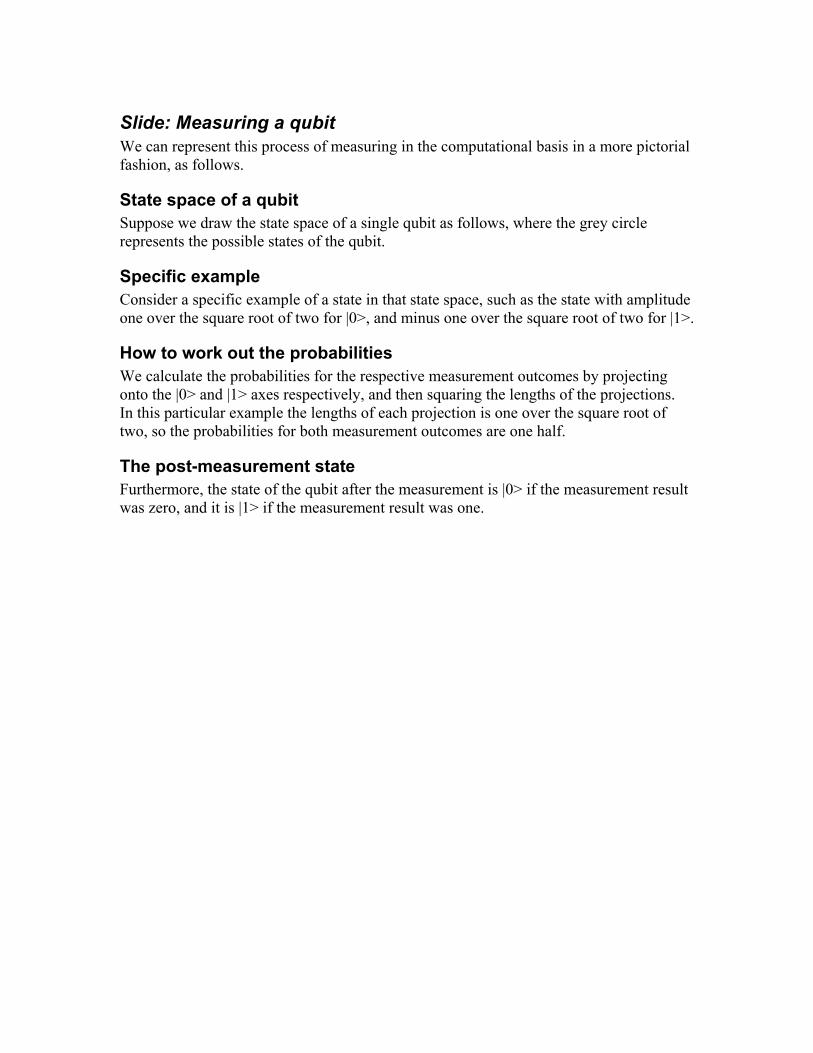
Slide: Measuring a qubit We can represent this process of measuring in the computational basis in a more pictorial fashion, as follows.

State space of a qubit Suppose we draw the state space of a single qubit as follows, where the grey circle represents the possible states of the qubit.

Specific example Consider a specific example of a state in that state space, such as the state with amplitude one over the square root of two for |0>, and minus one over the square root of two for |1>.

How to work out the probabilities We calculate the probabilities for the respective measurement outcomes by projecting onto the |0> and |1> axes respectively, and then squaring the lengths of the projections. In this particular example the lengths of each projection is one over the square root of two, so the probabilities for both measurement outcomes are one half.

The post-measurement state Furthermore, the state of the qubit after the measurement is |0> if the measurement result was zero, and it is |1> if the measurement result was one.

Slide: More general measurements More generally, for a general quantum system it is possible to do a measurement which is a natural generalization of the description I’ve just given for qubits.

Introduce the orthonormal basis In particular, suppose we have quantum system with d-dimensional state space, and |e_1> through |e_d> is some orthonormal basis for the state space.

The rule for determining measurement probabilities Then, given a quantum state |psi> for that system, quantum mechanics tells us that it is possible to do what is called a “measurement of |psi> in the basis |e_1> through |e_d>”. The outcome of the measurement is a number j in the range 1 through d. Outcome j occurs with probability that is given by the magnitude squared of the inner product of the corresponding vector |e_j> with the quantum state |psi>, and squaring it.

Reminder of the rule for taking an inner product In this expression the inner product is just the usual inner product. In particular, if we write the quantum state |psi> with respect to the computational basis, as I’ve done here for the case of a qubit, then the inner product is just as shown. Note that some mathematicians use the reverse convention where the complex conjugate is applied to the components of the second vector; in quantum information science the complex conjugate is invariably applied to the components of the first vector.

Disturbance of the system Furthermore, just as in the case of measuring in the computational basis of a qubit, more general measurements unavoidably disturb the state of the system, leaving it in the state |e_j> corresponding to the measurement outcome.

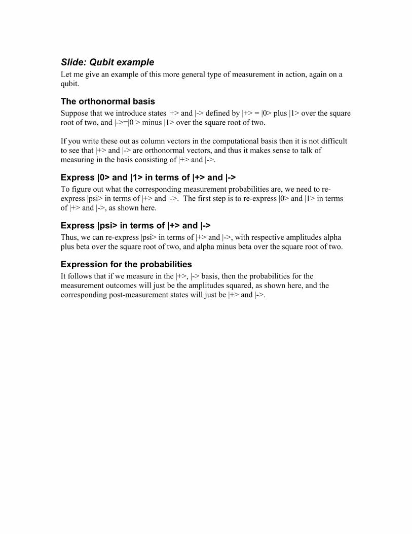
Slide: Qubit example Let me give an example of this more general type of measurement in action, again on a qubit.

The orthonormal basis Suppose that we introduce states |+> and |-> defined by |+> = |0> plus |1> over the square root of two, and |->=|0 > minus |1> over the square root of two. If you write these out as column vectors in the computational basis then it is not difficult to see that |+> and |-> are orthonormal vectors, and thus it makes sense to talk of measuring in the basis consisting of |+> and |->.

Express |0> and |1> in terms of |+> and |-> To figure out what the corresponding measurement probabilities are, we need to re-express |psi> in terms of |+> and |->. The first step is to re-express |0> and |1> in terms of |+> and |->, as shown here.

Express |psi> in terms of |+> and |-> Thus, we can re-express |psi> in terms of |+> and |->, with respective amplitudes alpha plus beta over the square root of two, and alpha minus beta over the square root of two.

Expression for the probabilities It follows that if we measure in the |+>, |-> basis, then the probabilities for the measurement outcomes will just be the amplitudes squared, as shown here, and the corresponding post-measurement states will just be |+> and |->.

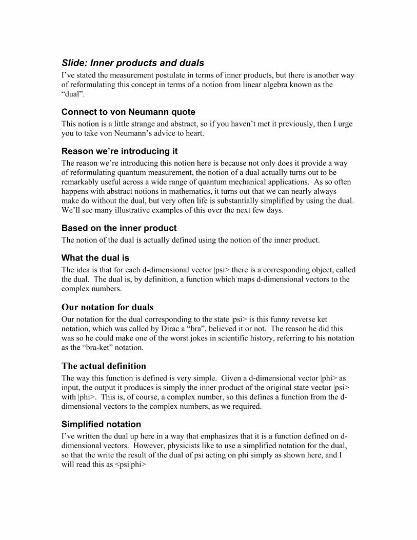
Slide: Inner products and duals I’ve stated the measurement postulate in terms of inner products, but there is another way of reformulating this concept in terms of a notion from linear algebra known as the “dual”.

Connect to von Neumann quote This notion is a little strange and abstract, so if you haven’t met it previously, then I urge you to take von Neumann’s advice to heart.

Reason we’re introducing it The reason we’re introducing this notion here is because not only does it provide a way of reformulating quantum measurement, the notion of a dual actually turns out to be remarkably useful across a wide range of quantum mechanical applications. As so often happens with abstract notions in mathematics, it turns out that we can nearly always make do without the dual, but very often life is substantially simplified by using the dual. We’ll see many illustrative examples of this over the next few days.

Based on the inner product The notion of the dual is actually defined using the notion of the inner product.

What the dual is The idea is that for each d-dimensional vector |psi> there is a corresponding object, called the dual. The dual is, by definition, a function which maps d-dimensional vectors to the complex numbers.

Our notation for duals Our notation for the dual corresponding to the state |psi> is this funny reverse ket notation, which was called by Dirac a “bra”, believed it or not. The reason he did this was so he could make one of the worst jokes in scientific history, referring to his notation as the “bra-ket” notation.

The actual definition The way this function is defined is very simple. Given a d-dimensional vector |phi> as input, the output it produces is simply the inner product of the original state vector |psi> with |phi>. This is, of course, a complex number, so this defines a function from the d-dimensional vectors to the complex numbers, as we required.

Simplified notation I’ve written the dual up here in a way that emphasizes that it is a function defined on d-dimensional vectors. However, physicists like to use a simplified notation for the dual, so that the write the result of the dual of psi acting on phi simply as shown here, and I will read this as <psi|phi>

This is our default notation for the inner product In fact, this notation has become the physicist’s default notation for the inner product. Very rarely will you see an explicit inner product between two vectors written in quantum mechanics. Instead, inner products are invariably written in terms of the dual of a state |psi> acting on the vector |phi>.

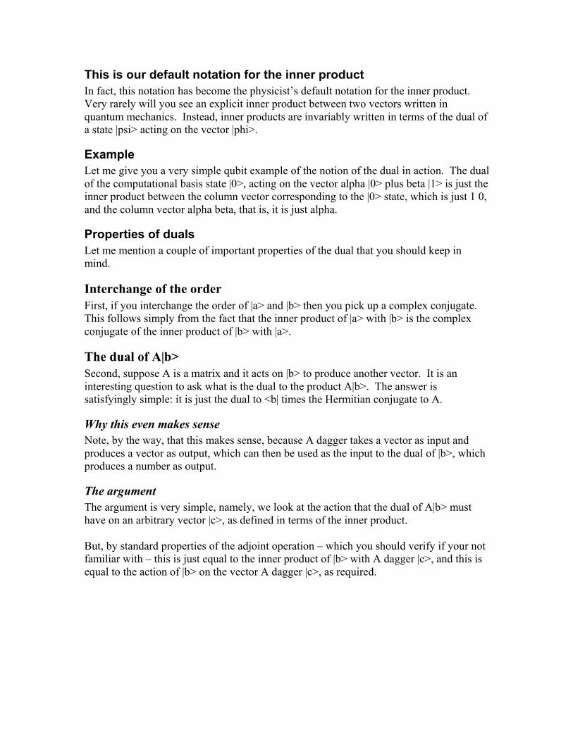
Example Let me give you a very simple qubit example of the notion of the dual in action. The dual of the computational basis state |0>, acting on the vector alpha |0> plus beta |1> is just the inner product between the column vector corresponding to the |0> state, which is just 1 0, and the column vector alpha beta, that is, it is just alpha.

Properties of duals Let me mention a couple of important properties of the dual that you should keep in mind.

Interchange of the order First, if you interchange the order of |a> and |b> then you pick up a complex conjugate. This follows simply from the fact that the inner product of |a> with |b> is the complex conjugate of the inner product of |b> with |a>.

The dual of A|b> Second, suppose A is a matrix and it acts on |b> to produce another vector. It is an interesting question to ask what is the dual to the product A|b>. The answer is satisfyingly simple: it is just the dual to <b| times the Hermitian conjugate to A.

Why this even makes sense Note, by the way, that this makes sense, because A dagger takes a vector as input and produces a vector as output, which can then be used as the input to the dual of |b>, which produces a number as output.

The argument The argument is very simple, namely, we look at the action that the dual of A|b> must have on an arbitrary vector |c>, as defined in terms of the inner product. But, by standard properties of the adjoint operation – which you should verify if your not familiar with – this is just equal to the inner product of |b> with A dagger |c>, and this is equal to the action of |b> on the vector A dagger |c>, as required.

Slide: Duals as row vectors There is a very useful way of understanding the dual in terms of row vectors.

Go through the calculation Suppose we expand vectors |a> and |b> in terms of the computational basis using amplitudes a_j and b_j. Then a straightforward calculation of the inner product shows that the action of the dual of |a> on |b> is the same as multiplying the row vector with components a_j^* by the column vector with components b_j.

Identification This suggests that we identify the dual of |a> with this row vector, and this is a point of view that we will frequently adopt.

Slide: Postulate 3: Rough form We’re now in position to describe the rough form of the third postulate of quantum mechanics. We will generalize this postulate a bit later, but for now it’s a good working approximation.

Two parts The postulate comes in two parts.

State the postulate: first part The first part states that if a quantum state |psi> in a d-dimensional state space is measured in the orthonormal basis |e_1> through |e_d>, then the probability of getting outcome j is given by this formula, namely the squared magnitude of the action of the dual of |e_j> acting on |psi>. Restating in terms of inner products, the probability is just the magnitude squared of the inner product between |e_j> and |psi>.

State the postulate: second part The second part of the postulate states that after the measurement, the state of the quantum system will be the state |e_j> corresponding to the measurement result obtained from the measurement.

Why this postulate causes problems This postulate has probably caused more problems and concerns than any other element of quantum mechanics. It is the main reason you hear people complain about the conceptual difficulties in quantum mechanics. People worry about questions like “what physical processes constitute a measurement?”, “what is a measuring device, anyway”, and “why is there randomness present in the postulates?”

How we’re going to respond These are all good questions, however in practice it has been found that they don’t affect how we use the theory very much. Nobody has ever found a concrete, specific situation where there is any difficulty in using the theory. For that reason, for most of the rest of this week we’re going to ignore the conceptual difficulties some people have with this postulate, and simply plough on ahead. The exception to this plan is that right now I’m going to explain where I think the conceptual difficulty lies, as best I can.

Slide: The measurement problem The problem I’m about to describe is often called the “measurement problem”, because it pertains to the status of the measurement postulate. I should stress, once again, that this problem has never caused anybody any difficulty in applying quantum mechanics to real problems. It’s just a question that many of us would like answered.

The process Imagine that you’ve got a quantum system. You want to perform a measurement on this system, so you bring it into contact with another system, the measuring apparatus. Those two systems now interact in the measurement process, producing some outcome.

What postulate 3 gives us Now, postulate 3 gives us a framework to describe this process in, according to dual vectors and so forth.

Expanded view However, the measuring device is just a quantum system, as was our original system. If we also include the rest of the universe in our description, then what we have is simply a very large closed quantum system. But postulates 1 and 2 prescribe a way of describing the evolution of such a closed quantum system.

Conclusion: quantum mechanics gives us two different ways of describing the process Thus quantum mechanics apparently gives us two different ways of describing this process.

The measurement problem The way I usually state the measurement problem is that it is to show that postulates 1 and 2 actually imply postulate 3.

A common response Some people will tell you that this has been done. I’ve had people tell me, point blank, that von Neumann and other people solved this problem back in the 1920s. However, if one goes and looks at those arguments, I believe they show nothing of the sort. All those old arguments attempt to do is show that the description given by postulate 3 is not inconsistent with that given by postulates 1 and 2, but this is hardly the same as deriving postulate 3 from postulates 1 and 2.

Caveat about my formulation of the measurement problem I should note, by the way, that I don’t really think that postulates 1 and 2 alone are sufficient to deduce postulate 3. For one thing, everything in postulates 1 and 2 is completely deterministic, and it is difficult to see how the probabilistic nature of postulate 3 could ever emerge from such postulates. So maybe something else needs to be added into the mix to solve the measurement problem.

Research Problem: solve the measurement problem In any case, as the first and likely most difficult problem of the week, I suggest that you solve the measurement problem. I should make it clear that this is likely a very difficult problem – some of the best minds in physics have spent a long time thinking about this problem, and they have not conspicuously succeeded.

What it has to recommend it as a problem On the other hand, I believe it has two major points in its favour as a research problem. First, it’s very important. Second, I believe that the eventual solution will be simple, but profound. That makes for a nice problem, in my opinion!

Slide: Revised postulate 1 That’s as much as I want to say for now about measurement in quantum mechanics. However, I’d like to briefly revisit postulate 1 and make it a little more precise.

Revised postulate The revised postulate states that to any quantum system there is associated a complex inner product space known as state space, and that the state of a closed quantum system is a unit vector in state space.

How it differs from the original This differs from the original definition in that I’ve replaced the term “vector space” with “inner product space”. I’m making the replacement to stress the point that the inner product is a very important part of the structure of quantum mechanics, since measurement is described in terms of inner products.

Viewpoint that this is merely quibbling This may seem like mere quibbling, because in finite dimensions vector spaces can always be equipped with an inner product. But in infinite dimensions that is not always the case.

Terminology: Hilbert space A related point has to do with terminology – physicist’s will often talk of the “Hilbert space” of their system. All they mean when they say this is state space. Once again, in infinite dimensions there are some additional technical niceties associated with Hilbert spaces, but we won’t need to worry about these niceties. For our purposes the way to think of state space is as a complex vector space with an inner product on it.

Slide: Multiple-qubit systems

Bridge from what we’ve done to what we’ll do We’ve talked a lot about single qubits. I want to talk now about how we can describe multiple-qubit quantum systems. How can we put the state spaces of those qubits together to form the state space for a two- or more- qubit system?

How to describe two-qubit systems The answer probably won’t surprise you very much. For a two-qubit system, what we do is to take all the possible two-bit strings, and we use them as computational basis states for the two-qubit space. A two-qubit quantum state is then a superposition over the four possible two-bit strings. Once again, the way to think of these computational basis states is as being essentially classical.

Measurement Of course, the computational basis states form an orthonormal basis, so in accordance with postulate 3 we can imagine measuring the system in that basis. If we do, then the usual rules tell us that the corresponding probability for getting the bit string (x,y) as the measurement outcome is just the modulus squared of the amplitude alpha_xy.

General state of n qubits These ideas generalize easily to n qubits. A general state of n qubits can be written as a superposition over computational basis states corresponding to every possible n-bit string.

What’s interesting: the classical description of such a state is very big Something that is very interesting about this is the fact that to specify a quantum state, it therefore requires specifying 2 to the power n different amplitudes. Even if we only specify them very roughly, this will still require an enormous amount of memory on a classical computer – at least 2 to the power n bits, and probably quite a bit more, to get a reasonable precision.

The intuition: it takes a lot more classical information to describe a quantum state than it does qubits This observation has led many people to believe that qubits in some sense “store more information than classical bits”, even though it is possible to prove that you can’t recover more than one bit of information per qubit. This idea was summed up most memorably by Carl Caves in his saying, “Hilbert space is a big place.”

This intuition as the basis for the idea that quantum computers might be more powerful than classical This idea was also the original basis for the idea that quantum computers might be more powerful than classical. The observation is usually attributed to Feynman, although the

idea had actually been proposed at least once before, by the Russian mathematician Yu Manin. In a book he wrote in 1980 Manin has a passage on exactly this subject, where he makes the point that we might need a mathematical theory of quantum automata, since the quantum state space grows exponentially, compared with the linear growth of the classical state space, and he proposes that the behaviour of the system might be much more complex than its classical simulation. There’s an amusing postscript to this story. I first heard about this quote of Manin’s from Alesha Kitaev, who had read Manin’s book. A long time after the book was written, Kitaev pointed the quote out to Manin, who had forgotten that he’d ever made such a comment in print, despite the fact that in the last few years he had become interested in the theory of quantum computation!

Slide: Postulate 4

What the fourth postulate tells us More generally, the fourth postulate of quantum mechanics tells us how to combine the state spaces of different quantum systems to get the state space of the composite system.

How I want to approach this: not to get too hung up on tensor products Now, before I state the fourth postulate I want to warn you that it contains a notion from linear algebra, the so-called “tensor product”, that some of you may not be familiar with. I don’t really want to get too hung up on describing the tensor product in detail. If you’ve never seen the tensor product before, rather than give you a rigorous definition, I’d rather became familiar with it simply by watching the way I work with it over the next lecture or so. You can then go back and study the rigorous definition to your heart’s content, if you so desire.

State the fourth postulate Without further ado, the fourth postulate states simply that the state space of a composite quantum system is just the tensor product of the state spaces of the individual systems.

Example: Two-qubits Let me give you an example of what this means. If we take two qubits then the state space is just the tensor product of the state spaces of the individual qubits, that is, it is the tensor product of two two-dimensional complex vector spaces. It turns out that this is essentially just the four-dimensional vector space I described on the previous viewgraph.

Computational basis states The way to think about the tensor product is by looking at a basis for the state space. The way an orthonormal basis for the tensor product space is formed is by forming objects which we call “tensor products” of orthonormal bases for the individual systems. The tensor product symbol is this funny times sign with a circle around it, shown here. Thus, for two qubits, the basis states for the two qubits correspond to these four objects, |0> tensor |0>, |0> tensor |1>, |1> tensor |0>, and |1> tensor |1>. A variety of shorthand notations are used, as I’ve shown here, including the notation I used on the last viewgraph, just writing the tensor product of |0> with |0> as |00>. The reason the tensor symbol is often written is simply to remind people that the tensor product is the construction being used, and that it has some very specific properties.

Properties Exactly what those properties are is not something you should worry too much about at this point – if you’re not familiar with the tensor product you should glance at this list now, and then look back if you’re ever uncertain. Let me run quickly through the list. First, we can pull complex numbers out of the tensor product to stand in front of the tensor product of two vectors. Second and third, the tensor product distributes across both the first and second entries. That’s a quick survey of the properties; the thing to do is to work through some examples of the tensor product in action, and get a feel for it that way.

Slide: Some conventions implicit in Postulate 4

State the fact There are some conventions implicit in postulate 4 that need to be spelt out in order for it to be possible to apply the postulate to problems. These implicit conventions are extremely natural, and are not usually stated in the postulate, but they form a kind of unwritten coda to the postulate that you should be aware of.

From components to Alice and Bob Rather than continuing to talk about the different components of the composite system, I’m now going to switch to more anthropomorphic language, and refer to the systems belonging to Alice and Bob. Of course, Alice and Bob are just labels – we don’t really need human observers around. However, they are easier to talk about than system A, system B, and so on. Furthermore, as David Mermin has pointed out, they also make available the rather nice apparatus of personal pronouns that English makes available.

First convention The first convention is that if Alice prepares he system in the state |a> and Bob prepares his system in the state |b>, then the state of the joint system is |a> |b>, that is, |a> tensor |b>.

Second convention The second convention is the converse of the first, namely, that if the state of the joint system is |a> tensor |b>, then we say that Alice’s system is “in” the state |a> and Bob’s system is “in” the state |b>.

Note on the phase ambiguity Notice, incidentally, that there is a phase ambiguity inherent in this convention, since |a> tensor |b> is also equal to e to the power I theta |a> tensor e to the power minus I theta |b> Of course, as we have already noted, a global phase is irrelevant in quantum mechanics, so this ambiguity is okay.

Third convention The third convention arises when Alice performs some dynamics on her system, described by a unitary operator U. The corresponding dynamics on the joint system is just U tensor the identity, where we define the tensor product for matrices as follows, namely the matrix A tensor the matrix B acting on the tensor product |v> tensor |w> is just A|v> tensor B|w>. The action of A tensor B on other states is just the linear extension of this definition.

Slide: Examples

Worked example To give you a better feel for this postulate, let me work through an extremely simple example. Suppose the quantum not gate is applied to the second qubit of the state root point 4 |00> plus root point 3 |01> plus root point 2 |10> plus root point 1 |11>. Then the resulting state may be found by applying the not gate to the second qubit of each of these states, giving root point 4 |01> plus root point 3 |00> plus root point 2 |11> plus root point 1 |10>.

Worked exercise In a similar vein, let me pose to you the worked exercise for this lecture. Suppose we have a quantum system in the state 0.8|00> plus 0.6 |11>. A not gate is applied to the second qubit and a measurement is performed in the computational basis. What are the probabilities for the different possible measurement outcomes?

Slide: Entanglement

Introduce the phenomenon There is a remarkable phenomenon associated with postulate 4 known as quantum entanglement.

Why we’re stopping Entanglement is going to be one of the key topics of these lectures, so it makes sense to introduce the concept here before coming back to revisit it later in the lectures.

Scenario Imagine Alice and Bob are each in possession of a single qubit. The joint state of these two qubits is the state |00> plus |11> over the square root of two.

Validity This state is, according to postulate 4, a perfectly valid state for the joint system of 2 qubits.

Peculiarity What’s peculiar about the state, however, is that it turns out to be absolutely impossible to write it in the form of a tensor product of a state |a> for Alice’s system, and a state |b> for Bob’s system.

Restate in more physical terms That is, it turns out to be impossible to understand this state as being a composite of a state of Alice’s system, and a state of Bob’s system.

The proof The proof of this fact is trivial: we suppose that psi can be written as a tensor product of such states, as shown here. Multiplying out, we see that the state must be of the form alpha gamma |00> plus beta gamma |10> plus alpha delta |0> plus beta delta |11>. The only way this can equal to |psi> is if this second co-efficient is zero, that is, either beta = 0 or gamma = 0. But in the first case the last co-efficient would vanish, and in the second case the first co-efficient would vanish, so this must be impossible. From this we conclude that psi cannot be written as a tensor product.

How we describe such states We describe such states as being “entangled states”, since they cannot be understood in terms of Alice’s and Bob’s individual systems, but rather embody some joint property of the system.

Our label for this particular state We will call this particular state the “Bell state”, or “EPR state”, for historical reasons.

Why this phenomenon is strange when viewed from a classical perspective From the point of view of our classical intuition entanglement is very strange. Given a physical object like a chair or a table we’re used to being able to give, at least in principle, a detailed description of the physical state of the chair. The phenomenon of entanglement indicates that it may not be able to assign a precise state to the chair, that it may only make sense to assign a precise state to a larger entangled system including the chair as just a component.

Schroedinger’s comment The phenomenon of entanglement was first pointed out in a paper by Erwin Schroedinger in the 1930s. He was so impressed by it that he called it not one, but rather the characteristic trait of quantum mechanics, the one that enforces its entire departure from classical lines of thought.

Our point of view Our point of view will not be far from this. Entanglement is one of the key concepts at the heart of quantum information science, and is exploited in many quantum information processing protocols. We’ll be seeing a lot of this “Bell state”, and of more complex entangled states.

Slide: Summary of the postulates Let me conclude this lecture with a single viewgraph summarizing all the postulates of quantum mechanics. There are only four. The first tells us where quantum states live, and what they are, for closed systems. The second postulate tells us how the quantum state of a closed system evolves in time. The third postulate tells us how we can measure the state of a quantum system. Finally, the fourth postulate tells us how the state space of a composite system is related to the state spaces of its components. These four postulates are all there is to quantum mechanics. Everything else depends upon the details of specific physical situations. I’ve taken you on a bit of a whirlwind tour of quantum mechanics up to this point. What I’m going to do in the next lecture is work through some examples of these postulates in action. These examples will hopefully be both interesting in their own right, and also useful as concrete examples of how to apply the postulates of quantum mechanics.

Lecture 2: Quantum Mechanics II

Slide: Overview of the lecture

What we’ve just done We’ve just spent a lot of time discussing the basic postulates of quantum mechanics, without giving a lot of examples.

What we’re now going to do: examples I want to remedy that now, by working through some simple, illustrative examples of quantum mechanics in action, as applied to the quantum information science. In particular, I’m going to discuss two of the most basic and important protocols of quantum information science, superdense coding and quantum teleportation.

Revised form of the postulates I’m also going to revisit postulate 2, about the dynamics of closed quantum systems, and postulate 3, about measurement, and present them in a slightly more refined form.

More Dirac notation I will also take this opportunity to introduce a few more conventions and examples of the Dirac notation.

Philosophy of quantum information science Finally, I want to talk a little about the philosophy underlying quantum information science: what it hopes to achieve, and how it hopes to achieve that.

Slide: Superdense coding Without further ado, let me introduce superdense coding.

Motivation in terms of Alice and Bob The motivation for superdense coding comes from the following scenario.

Alice and Bob Two parties, usually known as Alice and Bob, live a long way away from one another.

The information Alice has in her possession Alice has in her possession 2 classical bits of information, that I shall denote a and b.

The qubit Alice has in her possession Alice also has a single qubit in her possession. This is an isolated qubit, that has never been in contact with the rest of the world.

Question: can both bits be sent on the qubit? Consider the following question: is it possible for Alice to perform an operation on her qubit, determined by the two classical bits a and b, then transmit the qubit to Bob, and have Bob perform a measurement on the qubit that reveals to Bob the value of the two bits in Alice’s possession.

Succinct version of the question That is, can Alice and Bob transmit 2 classical bits of information using only one quantum bit?

Answer Unfortunately, the answer to this question is no. It turns out that we can prove that it is not possible to transmit more than one classical bit of information per quantum bit. This is perhaps slightly surprising, given that it took two complex numbers to describe the state of a qubit, but it is nonetheless true, and a consequence of the restrictions postulate 3 places on the measurements we can perform on the qubit.

Slide: Superdense coding

What superdense coding is Despite this impossibility, the superdense coding protocol is a protocol that enables something very similar to be done.

The resolution I’m going to use in discussing the protocol On this viewgraph I’m going to explain what the protocol accomplishes, and to give you a rough description of how the protocol works. On the next viewgraph I’ll give you the full quantum mechanical details.

How the protocol starts The protocol starts with two qubits in Bob’s possession. Bob locally prepares the two qubits in some joint state of his choosing.

Bob sends his qubit to Alice Bob sends his qubit over to Alice

What Alice does Alice then applies a local operation to the single qubit now in her possession, which changes the joint state of the system. The operation she chooses to do is determined by the values of a and b.

Sending it back and measuring Alice then sends the qubit back to Bob, who is now able to perform a measurement that reveals the value of a and b.

Summarizing The process I’ve just described is actually possible, and the procedure used to do it is called superdense coding. It’s a remarkable procedure, because Alice only ever comes in contact with one qubit, yet still manages to convey two bits of classical information. It’s also a very good but simple example of quantum information processing in action.

Slide: Superdense coding

What we’re now going to do Let me now describe the superdense coding procedure in detail.

The state Bob creates Bob creates the two qubit state which is an equal superposition of |00> and |11>, with amplitude one over the square root of two for each state.

Name the state and emphasize its important This state, by the way, is quite an important quantum state, and we’ll be seeing a lot of it. It’s often called the Bell state, or sometimes the EPR state, after Einstein, Podolsky and Rosen. These were four of the first people to realize what interesting properties states like this one can have. Qubits prepared this way are called a Bell pair or EPR pair.

Sending of the qubit Bob now sends one half of the Bell pair over to Alice.

What Alice does What Alice does to the qubit depends on what value of a and b she has.

Case: a=0, b=0 The first case is when a=0 and b=0, in which case Alice does nothing to her qubit, leaving the joint state as it was.

Case: a=0, b=1 The second case is when a=0 and b=1, in which case Alice applies the Z gate to her qubit. Recall that the Z gate takes the |0> state to |0>, while it takes the |1> state to minus |1>. To understand the action of the Z gate on this state then, we simply need to apply it to the first qubit of this state, in a linear fashion. We see that the first term is left alone, because Z acting on |0> does not change anything, while the second term picks up a minus sign, because Z acting on a |1> gives minus |1>.

Case: a=1, b=0 When a =1 and b=0, Alice applies the X gate to her qubit. Recall that this is just the not gate, which interchanges |0> and |1>. Thus, the first term |00> becomes |10>, and the second term |11> becomes |01>.

Case: a=1, b=1 In the final case, a = 1 and b=1, Alice applies first the Z gate, then the X gate to her qubit, and you can easily go through this to see that resulting state is |10> minus |01> over the square root of two.

Sending the qubit back The next step of the protocol is simply for Alice to send the qubit back to Bob, so that both qubits are in his possession.

The measurement step Bob now introduces a measuring device, and performs a measurement of the quantum state.

Why these four states can be distinguished Now, it is not necessarily obvious that Bob can perform a measurement that distinguishes these four states. However, a simple calculation will show that these four states are, in fact, orthonormal to one another, and thus can be distinguished by a quantum measurement.

Name: the Bell basis Indeed, these four states come up so frequently that they are given a name: they are known as the “Bell basis” of four qubits, and it is by measuring in the Bell basis that Bob is able to distinguish these four states, and thus to determine the value of Alice’s two bits of classical information.

Slide: Superdense coding and the interchangeability of physical resources

The significance of superdense coding Now that we’ve seen how superdense coding works, I want to talk a little more about why it’s significant. In itself it’s not that significant – it’s quite likely that it will never be terribly important as a scheme for communication. But we can learn important things about how to think about quantum information from superdense coding.

Interchangeability of physical resources One way of thinking of superdense coding is as a statement about the interchangeability of different physical resources.

Statement of the inequality In particular, the superdense coding protocol tells us that having a shared “ebit” of entanglement, that is, the Bell state, together with the ability to send a single qubit of communication, will always allow us to communicate two bits of classical information.

Disclaimer It is, perhaps, dangerous to take such inequalities too seriously, however, they are a useful way of thinking about processes such as superdense coding. We’ll come back and explore this point of view further with quantum teleportation.

Slide: Worked exercise on superdense coding Let me now state the worked exercise for this lecture, namely, to determine what happens if the initial state shared by Alice and Bob in the superdense coding protocol is changed to the state |01> minus |10> over square root of 2. All the actions performed by Alice and Bob are kept the same, including Bob’s final measurement.

Slide: Revised form of postulate 3

Bridge between superdense coding and teleportation In order to describe quantum teleportation, however, I’m first going to need to revisit the third postulate of quantum mechanics, and refine it a little. You might recall that in the last lecture I said that we’d left the postulate in a slightly rough form. We’re now going to remove that roughness.

Recall the first part of the postulate Recall that the postulate tells us that if we measure the state |psi> in an orthonormal basis |e_1> through |e_d>, then the outcome of the measurement will be j with probability given by the squared magnitude of the inner product between |e_j> and |psi>.

Recall the second part of the postulate Furthermore, if that measurement outcome occurs, then the post-measurement state of the system is just |e_j>.

What’s wrong with this formulation of the postulate? What’s wrong with this formulation of the postulate? The answer is, nothing, as far as it goes. The problem is that it doesn’t go far enough in describing the class of measurements that can be performed in quantum mechanics.

Explain the problem In particular, imagine that we have a quantum system in our possession, which we’ll call system A, and we perform a measurement on that system in the basis |e_1> through |e_d_A>, where d_A is the dimension of system A. Imagine, however, that system A is just part of a larger quantum system, containing two components, system A and system B. The question is, how do we describe the measurement in terms of the joint system AB. With the measurement postulate as currently formulated, there is no way of doing this, since the number of outcomes of a measurement on a quantum system must always be

exactly equal to the number of dimensions in that system’s state space, as we have currently formulated the postulate.

Slide: Revised measurement postulate

How the solution works The solution to this problem is to replace postulate 3 with a slightly revised postulate in which, instead of measuring a quantum state and resolving it into one of a set of orthonormal states, we resolve it into one of a set of orthonormal subspaces.

Example of what I mean by this I’ll be more precise about what I mean by this in a minute, but for now you can understand the principle by imagining that I have a quantum system with a three-dimensional state space, and an orthonormal basis |e_1>, |e_2>, |e_3>.

Expanding the state Now, of course, an arbitrary state |psi> can be expanded in terms of this orthonormal basis, as shown here.

How an old measurement would work The way I’ve been describing things up to now, a quantum measurement would determine which of these three states the system was in.

How the revised measurement would work: breaking up the state space However, with the revised postulate, it becomes possible to do another type of measurement. In particular, we can break the state space up into two parts, one part spanned by |e_1> and |e_2>, and the other part spanned by |e_3> alone.

How the revised measurement would work: doing the measurement It would then be possible to do a measurement checking to see whether the quantum system was in the space spanned by |e_1> and |e_3>, or if it was in the space spanned by |e_3> alone.

More generally More generally, given a decomposition of the state space into subspaces V_1 through V_m of this sort, it would become possible to ask which of those subspaces are we in?

Slide: Revised measurement postulate Material to be added, as the exact content is still uncertain.

Slide: Revised measurement postulate Material to be added, as the exact content is still uncertain.

Slide: Example of a two-outcome measurement on a qutrit Material to be added, as the exact content is still uncertain.

Slide: Example: Measuring the first of two qubits Material to be added, as the exact content is still uncertain.

Slide: Example: Measuring the first two of three qubits Material to be added, as the exact content is still uncertain.

Slide: Teleportation

Segue We are now in position to discuss the quantum teleportation protocol.

Alice’s qubit, and transmission to Bob The basic idea is that Alice has in her possession a single quantum system that she wants to transmit to Bob.

No quantum communication channel Unfortunately, transmitting quantum states is hard, and there is no quantum communications channel that will allow Alice and Bob to do this transmission.

Why doesn’t Alice just tell Bob what her state is? Why doesn’t Alice just tell Bob what her state is? There are two answers to this question. The first is that describing the state of even a single qubit means specifying two complex amplitudes, to arbitrary precision, which requires an infinite amount of classical information. Second, Alice may not even know what her state is, in which case the laws of quantum mechanics prevent her from determining the state.

What can Alice and Bob do? What can Alice and Bob do? An answer is provided by the quantum teleportation protocol.

How I will describe teleportation I will describe teleportation using a similar approach to that I took for superdense coding, first outlining the steps of the procedure, and then returning for a second pass, describing the procedure in detail.

Victor and the preparation of entanglement step The idea is that there is another party, Victor. A long time in the past, Victor has prepared two qubits locally in a quantum state, and transmitted one of those qubits to Alice and one to Bob.

Slide: Teleportation

Alice’s measuring device Alice now introduces a measuring device and performs a joint measurement on her two qubits, producing a two-bit measurement outcome, which I’ve shown here as 01. It may not surprise you to learn that the basis we’re going to measure in is actually the Bell basis of the two qubits in Alice’s possession.

Transmission of the measurement result She then transmits the measurement result over to Bob. She can do that without a quantum communications channel; all she needs is a radio transmitter, or some other form of classical communications channel.

Final step of the protocol The final step of the protocol is for Bob to apply some operation to his qubit, with the operation applied depending on which measurement result Alice sent to him.

Resulting state The result of this final operation by Bob is that his qubit ends up in exactly the same state as Alice originally had in her possession! That is, Alice and Bob have successfully teleported a qubit from Alice to Bob.

Slide: Teleportation

More detailed description Let me now give a more detailed description of the teleportation protocol.

Restriction to qubits I am going to suppose, for simplicity, that all the systems involved in the protocol are qubits, but the protocol is easily generalized to higher-dimensional systems.

Alice’s state I will suppose that Alice’s state is an arbitrary single-qubit state, alpha |0> plus beta |1>.

Victor’s preparation Victor’s initial state preparation is to take two qubits and prepare them in the Bell state |00> plus |11> over the square root of two.

Sending the qubits off He then sends the respective qubits off to Alice and Bob.

Rewriting the state Let me now rewrite the joint state of Alice and Bob’s system all in one location.

Expand the state out Furthermore, using the distributive property of the tensor product we can expand this out in the following form.

Why we rewrite the state Well, Alice is going to do a measurement of her two qubits in the Bell basis, so it would be good to rewrite this state in terms of the Bell basis on the first two qubits.

The case of |00> In the case of |00>, it can be rewritten as a linear combination of two elements of the Bell basis, with equal amplitudes one over the square root of two.

Other cases Similarly, it is a simple exercise to go through and rewrite all the other computational basis states in terms of the Bell basis.

Next idea is to substitute The next step is to substitute these expressions for the computational basis states to rewrite this state in terms of the Bell basis on the first two qubits.

Slide: Teleportation

What happens when we rewrite in terms of the Bell basis When we do this substitution, we get the following rather remarkable expression.

What we’ve done up to this point Notice that, up to this point, we haven’t actually done anything except for algebra.

The measurement What happens next is that Alice performs a measurement of her two qubits, in the Bell basis?

Equal probability, independent of the state Alice is going to send Well, first of all, notice that measurement probability for each Bell state is just the square of the amplitudes, which happen to be one half in each case, so all the probabilities are the same, ¼, independent of the state being teleported.

Case: Second element of the Bell basis Suppose Alice finds that her qubits are in the second state of the Bell basis, corresponding to this second term, here.

What Bob’s conditional state is Well, in this case, the conditional state of Bob’s system is just alpha |0> minus beta |1>.

Bob applies Z But suppose Bob were to apply the Z gate to his system. Recall that the Z gate leaves |0> alone, and changes |1> to minus |1>. Thus, the sign of |1> will be flipped around, and Bob will end up with the state alpha |0> plus beta |1>, which was the original state of Alice’s system.

Case: other elements of the Bell basis Similar things happen in the other three cases. For example, when Alice gets the measurement outcome corresponding to the first element of the Bell basis, it turns out that Bob’s conditional state is exactly Alice’s original state, and he doesn’t need to do anything to complete the teleportation. If Alice gets the third Bell state, then Bob can fix up his state by applying an X gate, while if Alice gets the fourth, then Bob completes teleportation by applying first X then Z to his qubit.

Summary In any case, no matter what the outcome of Alice’s measurement, Bob will end up in possession of the state originally belonging to Alice.

Comment on the interesting features of teleportation Teleportation has many interesting and remarkable features

Apparent violation of light-speed limit First, you might be tempted to wonder whether or not teleportation violates the rule saying that information can’t be transmitted faster than light. After all, doesn’t Alice’s measurement cause Bob to instantaneously obtain Alice’s state |psi>, or, at least, something related to it. It turns out that, in fact, it is not possible for Alice and Bob to use this effect to communicate faster than light. In particular, it can be shown – and we will do this explicitly later in the week – that unless Alice transmits the result of her measurement to Bob, then it is impossible for Bob to extract any information out of his qubit. Thus, the speed of information transmission using teleportation is limited by the speed with which Alice can transmit her measurement result to Bob, and so far as we know, that is only light speed, so there is no possibility of using teleportation to do something faster.

“Infinite information” with only two classical bits Another interesting feature of teleportation is that it only involves two bits of classical communication. That’s rather remarkable, when you consider that giving a classical description of Alice’s quantum state would require an infinite amount of classical information.

Blind nature of the protocol It’s even more remarkable when you consider that Alice didn’t even need to know what her quantum state was to perform the protocol. The rules of quantum mechanics prevent her from ever determining the state of her system, yet she and Bob still succeed in transmitting that state, using just two bits of classical information and a pre-shared Bell state.

The fact that no information about the state is carried by the two classical bits Another remarkable feature of teleportation is that the probabilities for the measurement outcomes don’t depend upon the state being teleported. This is really rather remarkable: it means that a person who intercepted the classical communication from Alice to Bob would not be able to infer anything about the identity of the state being teleported from that information. That is, the classical message from Alice to Bob contains, in some sense, no information about identity of the state being teleported!

Utility later in the week That’s a rather long list of remarkable and somewhat mysterious features. I’d like to be able to give you a pat explanation of why this should all be rather expected, but at the present point I can’t, and I don’t think anybody else can. What is the case is that teleportation is certainly important, both because of remarkable properties like those I’ve just listed, and also because it turns out to be incredibly useful in a wide variety of other contexts. In particular, later in the week we’ll actually see that teleportation can be used as a key primitive operation in both quantum computation, and quantum error-correction.

Slide: Teleportation and the interchangeability of physical resources

Analogy with superdense coding I’d like now to talk about teleportation from a slightly different point of view, just as I did earlier with superdense coding, as a statement about the interchangeability of different physical resources.

Statement of the inequality In particular, we learn from the teleportation protocol that a shared ebit of entanglement, together with the ability to send two bits of classical information, enables the transmission of a single qubit.

Comparison with superdense coding We can compare this inequality with that we wrote earlier, for superdense coding, namely, that one ebit together with one qubit of communication allows two bits of classical communication.

Summary in one equation Comparing these two inequalities, we can even write a beautiful equality, namely, that, modulo having a shared ebit, one qubit of communication is completely equivalent to two bits of classical communication.

The utility of this point of view: algebraic inspiration The utility of this inequality-based point of view is that it can inspire us to think in an interesting way about quantum information processing – basically, using our “algebraic intuition” about inequalities and equalities to motivate the study of quantum information processing.

Motivation for a theory of entanglement and quantum information Indeed, if one is going to take such inequalities seriously, one might well ask questions like “what would correspond physically to a fraction of an ebit of entanglement?” and “what would a fraction of an ebit allow me to do?” Such questions motivate the quantitative theory of entanglement, and more generally, of quantum information theory, as we shall discuss later in the week.

Slide: the fundamental program of information science

How these questions fit into a larger program for doing information science These sorts of questions are really all part and parcel of a more general program for doing information science both quantum and classical.

My name: the “fundamental program of information science” I’m going to give this program a rather grandiose name, the “fundamental program of information science”. I should mention, by the way, that the following formulation is actually due to Ben Schumacher; other people have also proposed similar ways of looking at information science in the past, but I’m borrowing this specific formulation from Schumacher.

What the program is, in broad terms The program abstracts a framework that, with variations, can be used to understand how information science progresses. It is

The first step The first step of the program is to identify a physical process, like energy, time, bits, space, or perhaps shared entangled pairs, that can be used to do information processing.

The second step The second step is to identify an information processing task. In a classical context that might be something like data compression. In both classical and quantum contexts it could be information transmission. In a quantum context alone it might be teleportation, broadly defined to be the transmission of a quantum state using pre-shared entanglement and classical communication.

The third step The third step is to identify a criterion for successful completion of the information processing task.

The question Once we’ve done all three of these things we can ask the basic question of information science, how much of 1 is needed to do 2, while satisfying 3?

Examples Examples of this program abound.

Classical data compression For example, the classical theory of data compression identified a physical resource – bits – an information processing task – compressing the output from an information source – and a criterion for success – the ability to recover the original information from the

compressed version. Shannon then asked how much of 1 was needed to accomplish 2 while satisfying 3? Asking this question led directly to the concept of entropy, which is the fundamental concept of classical information theory.

Algorithms Or to take a much more complex example, in the theory of quantum computation, we start with a physical resource – qubits and quantum logic gates, and an information processing task, like factoring a large number, and ask how much of the physical resource is required to achieve the information processing task, with a high probability of success?

What this leads to History has shown that pursuing this program, and allowing quantum resources, has inspired the discovery of many interesting new ways of doing information processing, some of them quite superior to classical ways of doing information processing. Quite likely, this will continue in the future.

What is good about this Well, this is good news, of course, and the purely utilarian benefits of following the program are obvious – inventing new ways of doing information processing is certainly interesting, and probably of benefit to society.

“How to write a quant-ph” However, after describing this fundamental program in another lecture, another researcher in quantum information made some rather thoughtful remarks about the program. He felt that it captured the essence of much of the work in quantum information science very well, but summed his thoughts up in the half-admiring, half-disparaging phrase that this program is exactly what one needs to “write a quant-ph”.

Does this have a scientific benefit Underlying that remark was another question – is this program just about finding neat ways of doing information processing, or are we addressing fundamental scientific questions?

My answer My answer to this question is that the methodology of quantum information science is, in fact, a very powerful way to approach fundamental scientific questions, and I will point out numerous examples over the coming week.

Slide: What fundamental problems can be addressed by quantum information science?

Broad explanation of the answer to this question I’d like now, however, to explain in broad terms what fundamental problems can be addressed by quantum information science.

The story of the chess player To explain what quantum information science is all about, I want you to imagine that you’re one of the world’s great chess players, like Gary Kasparov, shown here.

Your challenger You’re introduced to a disreputable looking character who claims to know all about chess.

The fact that they do know the rules When you play a game against this person, you find that, indeed, they do know all the rules of the game, for the moves they make are always according to the rules of the game.

But their moves are absurd Nonetheless, their moves are absurd – they do things like sacrificing their queen for a pawn, and their rook for no apparent reason at all.

Your conclusion Thus, although the person knows the rules of chess, you conclude that they do not truly understand chess, (picture) in the sense that they are not familiar with any of the high-level principles, heuristics and rules of thumb that constitute a true understanding of chess, and which are familiar to any chess master.

Slide: Knowing the rules of quantum mechanics doesn’t mean we understand it

Make the analogy Similarly, just because humanity has known the rules of quantum mechanics for 80 odd years doesn’t mean that we truly understand quantum mechanics.

My claim My claim today is that, just as in chess, there are high-level principles implicit in quantum mechanics, and we must discover these principles before we can claim a reasonable understanding of quantum mechanics.

How to view quantum information science One way of viewing quantum information science is as an approach to the problem of discovering these principles.

Digression to Laughlin’s Nobel Prize Lecture Before I explain why that is the case, let me remind you of another field where some high-level principles of quantum mechanics have been discovered, with a quote from Robert Laughlin’s 1998 Nobel Prize Lecture.

Slide: quote from Laughlin’s Nobel Prize Lecture

Introduction Laughlin states that “I give my class of extremely bright graduate students, who have mastered quantum mechanics but are otherwise unsuspecting and innocent, a take-home exam in which they are asked to deduce superfluidity from first principles.”

His remarkable assertion He goes on to make the remarkable assertion that “There is no doubt a special place in hell being reserved for me at this very moment for this mean trick, for the task is impossible.”

Explanation of the assertion He explains this assertion with the remark that “Superfluidity, like the fractional quantum Hall effect, is an emergent phenomenon – a low-energy collective effect of huge numbers of particles that cannot be deduced from the microscopic equations of motion in a rigorous way and that disappears completely when the system is taken apart”, a viewpoint that he attributes to Phil Anderson’s well-known 1972 paper in Science, which argues that “More is different”.

Comment on the validity of the claim This is a remarkable claim, and not one whose validity I want to argue today, although I am sympathetic to it.

What everybody can agree on What I’m sure everybody can agree on is that phenomena like superfluidity and the fractional quantum Hall effect are not at all obvious from the principles of quantum mechanics, and that they are examples of complex quantum systems governed by a set of high-level principles implicit in the underlying rules of quantum mechanics.

Slide: How quantum information science offers an approach to the study of complex quantum systems

Bridge from the existence proof to the question of what quantum information science offers Having offered you my “existence proof” for complex emergent principles in quantum systems, I now want to discuss how quantum information science offers a general approach to the study of such complex quantum systems.

Difference from condensed matter physics Obviously, this approach is rather different to the methods of condensed matter physics used to study phenomena like the fractional quantum Hall effect, and I’d like to describe the path I see for quantum information science to offer an approach to the study of complex quantum systems.

Picture of all possible quantum processes Consider this heuristic picture of the space of all quantum processes.

Notion of complexity In this picture, moving from left to right indicates an increase in the notional “complexity” of a process.

Left-hand end: communication, crypto, and teleportation At the left-hand end we have relatively simple quantum processes, such as quantum communication, quantum cryptography, and quantum teleportation.

What happens when we follow the fundamental program of quantum information science Suppose now that we take these processes and follow the fundamental program of information science that I identified earlier – that is, we identify the physical resources that are being consumed by these process, and attempt to quantify the minimal resources that are required to successfully perform those processes.

How this leads to unifying concepts like entropy By following this program with relatively simple processes, like data compression, we are led to concepts such as the Shannon entropy, which have since been used to build up an understanding of more complex processes, like communication in the presence of noise, and networks of communication channels.

In the quantum case: concepts like entanglement In a similar way, in the quantum case following this program leads to the development of unifying concepts, of which I’ll mention just one right now – the quantitative theory of entanglement that I’ll speak about on Thursday.

The hope: that by understanding these we can gain insight into still more complex processes The hope, then, is that by following the fundamental program of information science we will develop many such insight-giving tools, like the quantitative theory of entanglement, and that these will then be used as a basis to gain insight into even more complex processes, like quantum algorithms, quantum error-correction, and maybe even processes not traditionally thought of as being information processing, like quantum phase transitions.

A few such connections have even been made A few such connections have already been made. Attempts have been made, with partial success, to explain the speed-up of quantum algorithms by the utilization of entanglement. The success of quantum error-correction is intimately related to the entangled properties of the states constituting the error-correcting code. And, as I will

briefly describe on Thursday, the theory of entanglement has resulted in new insights into quantum phase transitions.

Summary Thus, the hope is that by following the program of quantum information science we will gradually build up an arsenal of unifying concepts that will greatly enhance our general understanding of the behaviour of complex quantum systems.

Slide: A few quanta of miscellanea That just about wraps up the things I want to say about elementary quantum mechanics. There are just a few miscellaneous bits and pieces that I need to add.

What these things are, broadly These bits and pieces fall into two categories: bits of mathematical formalism that we will need later this week, and minor refinements or variations on the postulates of quantum mechanics.

How important is it that people master all this I realize that it’s been a long lecture already, and some of this material is a little overwhelming if it’s the first time you’ve encountered it. For that reason, let me say that it’s not all that important that you assimilate all this material in this one go. Just absorb as much as you can now, and then tonight attempt some of the exercises I will give you. It’s pretty basic stuff, but there is a lot of notation to absorb all at once.

Outer product notation for matrices The first thing I’m going to describe is a very useful and widely used piece of notation for matrices called the “outer product” notation. This is the last major piece of the Dirac notation that we shall need.

Spectral theorem With the outer product notation in hand, I’ll use it to describe a very useful representation theorem from mathematics about Hermitian matrices, known as the spectral theorem.

The trace operation I’ll also briefly remind you about a standard matrix operation, the trace operation, and some of its properties.

Digression: measurement I’ll also take this opportunity to go on a slight digression into the history of quantum mechanics, revisiting the measurement postulate from a slightly different angle. In particular, I’m going to present to you the form of the measurement postulate as you’ll see it given in older quantum mechanics textbooks. This form is equivalent to the form I’ve described. I’m describing it to you both for historical interest, and because in the

next lecture I’m going to use this revised form to ask an interesting question about physics, motivated by computer science.

Quantum mechanics in continuous time Finally, I’ll finish the lecture off by describing the second postulate of quantum mechanics to you in a slightly different form. The way I described it to you earlier today it describes how to relate the quantum state of a closed quantum system at two different points in time, namely, by a unitary operation on state space. Of course, physicists usually think in continuous time, and the more usual formulation of that postulate is in terms of a differential equation giving the continuous time behaviour. I’ll describe that form of the postulate.

Slide: The outer product notation

Purpose of the notation Let me describe for you an extremely useful notation for matrices known as the outer product notation.

Basic definition

|Psi> and <phi| Suppose |psi> and |phi> are two vectors, not necessarily quantum states.

Define |psi><phi| Then we can define a linear operation, that is, a matrix, acting on state space, which is denoted as |psi><phi|, as shown here.

The action By definition, the action of this operation on an arbitrary state |gamma> is to return the vector |psi>, but multiplied by the inner product of |phi> and |gamma>, as shown here.

Comment on the beauty of the notation We see here the beauty of the Dirac equation, in that the action of the outer product |psi><phi| is more or less obvious from the notation.

Comment on how we abuse notation Indeed, this leads us to abuse notation quite a bit: it is usual to regard this expression on the right-hand side in two different ways, either as the action of the outer product matrix |psi><phi| on the vector |gamma>, or else just as |psi> times the inner product between |phi> and |gamma>.

Example Let me give you a very simple example of the outer product in action. Consider the outer product |1><0| acting on an arbitrary state of a qubit. It just returns the state |1> multiplied by the inner product between |0> and the state of the qubit, in this case, alpha.

Connection to matrices It is helpful for understanding to connect the outer product to the matrix picture.

Write |a> and |b> in the computational basis In particular, suppose |a> and |b> are vectors which, when written in the computational basis, have amplitudes a_j and b_j, respectively.

Action on a computational basis state Then the action of the outer product |a><b| on a computational basis state which I denote |l> is just to return the lth amplitude for |b>, times |a>.

Compare with matrix notation Imagine, however, that we consider the matrix formed by doing regular matrix multiplication of the column vector with amplitudes a_l, and the row vector with entries b_l^*. If we consider the action of this matrix on a column vector with just a single 1 entry in the lth component, and zeroes everywhere else, then it returns b_l^* times the vector |a>

Conclusion Thus, we conclude that the matrix representation for the outer product |a><b| is just the matrix product of the column vector representing |a> and the row vector representing the dual <b|.

Slide: The outer product notation

Topic of the slide is examples We can now work through some illustrative examples of the outer product. Work through examples, as per the viewgraph.

Slide: The outer product notation

Advantages of the outer product notation One of the advantages of the outer product notation is that it provides a convenient tool to describe projectors, and thus, to describe quantum measurements.

Example To see this, recall the earlier example of a projection onto a two-dimensional subspace of a three-dimensional space spanned by orthonormal vectors |e_1>, |e_2> and |e_3>. The projector simply eliminates the component of any vector in the |e_3> direction.

See that |e_1><e_1|+|e_2><e_2| works the same way To see the connection to the outer product, just notice that the outer product |e_1><e_1| acting on this state returns alpha |e_1>, while the outer product |e_2><e_2| returns beta |e_2>.

Conclusion From this, we conclude that in fact the projector P must be equal to the sum of the outer product |e_1><e_1| with the outer product |e_2><e_2|

General result More generally, it is not difficult to prove that the projector P onto an m-dimensional vector space spanned by |e_1> through |e_m> is just given by the sum over all the outer products |e_j><e_j|.

Finally: two exercises Let me conclude this discussion of the outer product representation with two exercises for you to consider.

First exercise The first exercise is to find an outer product representation for the Pauli Y matrix introduced in the last lecture.

Second exercise The second exercise is to prove that if we take the Hermitian conjugate of the outer product |a><b| then we obtain the outer product |b><a|.

Slide: The spectral theorem

What the spectral theorem is There is a very useful representation theorem, the so-called spectral theorem, that is often very handy when dealing with Hermitian matrices.

What the theorem states What the theorem tells us is that any Hermitian matrix, A, may be diagonalized. That is, there is a unitary matrix U such that A is equal to U times a diagonal matrix times U dagger, where the entries of the diagonal matrix are just the eigenvalues of A.

Why this is useful The reason this theorem is useful is because it gives us an explicit representation for Hermitian matrices, a representation that is not possible for a generic matrix.

Why we’re going to put it in a slightly different form We’re going to use the outer product notation to put this theorem in a slightly different form, a form that is often better adapted to the needs of quantum mechanics.

Put diagonal matrices in the outer product form To translate the spectral theorem into the language of the outer product, observe first that the diagonal matrix appearing in the theorem can be written in the form the sum on j lambda j times the outer product |j><j|, where the vector |j> is just the jth computational basis state.

Substitution Substituting this expression into the spectral theorem, we see that A can be written as the sum on j lambda j times the outer product |e_j><e_j|, where |e_j> is defined to be U times the computational basis state |j>. Notice, however, that from this form, if we consider the action of A on |e_j> then we just get lambda_j |e_j> back, so |e_j> is just the eigenvector of A corresponding to the eigenvalue lambda_j.

Comment on the utility of this form and nomenclature This form, shown here, is a very useful form. Quantum information scientists often say that they are writing a matrix “in its diagonal form” when they write it in this form.

Write things in terms of projectors Finally, if collect up all the terms |e_j> corresponding to the same eigenvalue, then we see that this expression can be rewritten as the sum on j lambda_j times P_j, where P_j projects onto the eigenspace of lambda_j, and j now labels the distinct eigenvalues.

Comment on the utility of these two forms These last two forms are very frequently used in quantum information science.

Slide: Examples of the spectral theorem Let me run quickly through a couple of examples of the spectral theorem.

Z example First is the example of the Pauli Z operator which, in addition to being unitary, is also easily seen to be Hermitian.

Spectral form We showed earlier that the Pauli Z can be written in the form |0><0| minus |1><1|; this is, in fact, also the spectral decomposition of Z.

X example As another example, consider the X matrix. It is not so obvious what the spectral decomposition of X is. However, if we observe that the eigenvectors of X are given by the two states |plus / minus> defined to be either |0> plus |1> over the square root of two, or |0> minus |1> over the square root of two, then it is easy to check that the corresponding eigenvalues of plus and minus 1.

How it all works out According to the spectral theorem X should therefore be equal to the outer product |+><+| minus the outer product |-><-|. I will not go through the details here explicitly, but you are welcome to run through them later.

Slide: The trace operation Another piece of mathematical technology that we’ll need is the trace operation. I assume that most of you have already met the trace, and will just briefly run over its basic properties now.

Definition By definition, the trace of a matrix is just the sum of its diagonal elements.

Example: X For example, the trace of the X matrix is just zero plus zero, which is zero.

Example: I While, for the two by two identity matrix, the trace is just one plus one, which is two.

Cyclicity A very important property of the trace is the so-called cyclicity property, which states that the trace of AB is equal to the trace of BA, for any two matrices A and B. The proof of this is a simple algebraic exercise, that you can follow through later.

Trace of an outer product Another important formula is for the trace of an outer product. I leave it to you as an exercise to prove that the trace of the outer product of |a> and <b| is just the inner product between |a> and |b>.

Slide: A revised form of postulate 2 Let me change topics now and talk about a slightly different form of postulate two.

Recall the postulate Recall that the second postulate of quantum mechanics stated that the time evolution of a closed quantum system is described by a unitary transformation.

Restate That is, if the state at time t_1 is |psi> then the state |psi’> at a later time t_2 will be related to the initial state by a unitary transformation U. That unitary transformation depends only on the times t_1 and t_2, and not on the states |psi> and |psi’>.

This will be fine for most of our applications This form of the postulate is fine for most of the applications we’ll be concerned with.

Difficulty and the resolution: need for a continuous-time description However, physicists currently believe that time is a continuous variable, and it would be nice to have a form of the postulate that is better adapted to the description of quantum systems evolving in continuous time.

What we’re going to do, and when this will be useful Over the next couple of viewgraphs I’m going to explain how this postulate can be formulated in continuous time. This is both interesting in its own right, and will be useful in the discussion of real physical systems, in tomorrow’s lecture by Andrew White, and later in the week in the research lectures.

Slide: A revised form of postulate 2

State the revised postulate According to the revised form of the postulate, the evolution of the state vector of a closed quantum system is controlled by an equation known as Schroedinger’s equation.

Schroedinger’s equation Schroedinger’s equation is a differential equation relating the time rate of change of the state vector to the state vector itself, but with a multiplying prefactor, known as the Hamiltonian of the system.

What the Hamiltonian does You can think of the Hamiltonian as capturing the dynamics of the system. It plays a similar role to the unitary operation appearing in the other formulation of postulate 2.

Quantum mechanics does not specify the Hamiltonian Note that quantum mechanics does not specify the exact form of the Hamiltonian – that is a job for specific physical theories.

What quantum mechanics does do What quantum mechanics does do is to constrain the class of allowed Hamiltonians to be Hermitian matrices acting on the state space of the system.

Figuring out the Hamiltonian is hard In general, figuring out the Hamiltonian for any specific system is actually pretty difficult, but physicists have a lot of rules of thumb for doing so.

How to approach all of this In fact, two of the major things that physicists have done over the last 80 years is (a) figure out Hamiltonians for systems of interest; and (b) figured out how to solve this equation. I can’t hope to teach you how to do this in a week, and am not going to try. What you should do is appreciate the conceptual structure underlying all this: physicists figure out Hamiltonians for systems, whose time evolution is then governed by the Schroedinger equation.

Terminology: energy Let me explain a very interesting and perhaps slightly confusing piece of terminology to you. The eigenstates of the Hamiltonian H are often referred to as the “energy eigenstates” of that system, and the correspond eigenvalues are referred to as energies.

What does this have to do with energy? What on earth does this have to do with our familiar, everyday notion of energy, you might ask? That’s a good question, and it’s not one that I’m going to answer. Instead, I want you to take it on faith that the allowed energies for a quantum system correspond exactly to the eigenvalues of that Hamiltonian, and when we say that a system is in a state with a particular energy, we mean that it is in the corresponding energy eigenstate.

Example: a qubit Hamiltonian Let me give you a very simple example of the sorts of Hamiltonians that often arise.

State the Hamiltonian It is a Hamiltonian for a single qubit, and it is just a number, omega, times the Pauli X operator. Notice that the Hamiltonian is Hermitian, and it has eigenvalues plus and minus omega, which we refer to as the “energy levels” for this system. The corresponding energy eigenstates are just the eigenstates of X, |0> plus |1> over the square root of two, and |0> minus |1> over the square root of two.

Slide: Connection to the old form of postulate 2 Let me finish up this lecture by explaining how this new form of postulate 2 connects to the old form of postulate 2 that I gave in the last lecture.

State the solution to Schroedinger’s equation Because the Hamiltonian is a constant matrix, it’s not difficult to solve Schroedinger’s equation exactly. When we do this, we discover that the state of a system at time t is related to the state at time 0 by the exponential of minus I times H times t.

What use is this solution? Well, I say solve, but in fact it’s difficult to get much information out of this solution unless you can compute this matrix exponential exactly, which is quite difficult, in general.

The good news: this matrix is unitary! However, the good news is that if we define U to be the matrix relating the initial to the final state, then it is, in fact, possible to prove that U is unitary, which provides the connection to the old form of postulate 2.

How we should think about postulate 2 For most of this week, the way we’re going to think about postulate 2 is in terms of the unitary formulation. For applications to quantum information and computation you mostly don’t need to worry about Hamiltonians. The reason is because in theoretical

quantum information science you just assume as given the ability to perform certain unitary operations, and see what else this enables you to do. I did this in superdense coding and teleportation, for example, where I just assumed that Alice and Bob can apply the Pauli gates to their qubits. For this reason we won’t need to worry much about a problem that worries physicists a lot, namely, finding explicit solutions to Schroedinger’s equation.

Lecture 3: Computer Science

Slide: Title slide

Focus of this lecture The purpose of this lecture is to introduce some fundamental notions of computer science. The focus of this lecture will be rather different from this morning’s lecture. Quantum mechanics is fundamental to everything we do, so it is important to understand in detail the basics of quantum mechanics. By contrast, notions from conventional computer science are mainly interesting as a source of inspiration; we don’t actually need to know all the details in order to draw inspiration. Thus, this lecture will focus more on some big picture ideas related to computer science, and less on specific technical details.

Notion of computational complexity That said, there are two things you should come away from the lecture having understood. The first is an understanding of what we mean when we talk about the computational complexity of a problem, and an understanding of the so-called computational complexity classes, which are just collections of problems all of which share some common feature in terms of the computing resources required to solve those problems.

Reversible computation Second, you should come away with some understanding of how a classical computer can be constructed in such a way that the computations done on the computer are reversible. That is, every step of the computation can actually be inverted, unlike a regular computer, where information is being lost all the time, so it is impossible to reverse the computation. It turns out that quantum computations are inherently reversible, which is why we are interested in studying reversible classical computation first.

Slide: History of computer science

Historical introduction using fundamental questions I’m going to begin with a little bit of historical background, looking at some of the fundamental questions underlying the modern field of computer science.

Hilbert’s problem One of the major strands of thought underlying computer science begins with the great German mathematician David Hilbert, who asked whether or not there is a general algorithm to determine whether a mathematical conjecture is true or false.

Hilbert’s guess as to the answer Hilbert thought the answer was yes, and that to prove this all that would be required is to construct such a procedure explicitly.

Church and Turing’s shocking announcement The world was shocked, therefore, when Alonzo Church and Alan Turing announced that, in fact, no such procedure exists.

Concentration on Turing, rather than Church For the sake of concreteness, I’m going to concentrate on what Turing did, but Church did rather similar things, more or less independently.

Turing’s mathematical formalization of the concept of an algorithm What Turing did was to construct a rigorous mathematical definition capturing the hitherto rather vague concept of an algorithm. Turing asserted that his mathematically well defined model of a computer, now known as a Turing machine, captures exactly the class of processes that can be regarded as algorithmic.

The Church-Turing thesis This assertion, that the Turing machine captures the notion of an algorithm, is now known as the Church-Turing thesis, in Church and Turing’s honour, and it is absolutely central to computer science, for it provides a rigorous mathematical foundation on which computer science can be built. It might be compared to, for example, Galileo and Newton’s achievement in putting physics on a mathematical basis.

Ad hoc nature of the justifications for the CT thesis A major drawback, however, of the Church-Turing thesis is that Church and Turing’s justifications for it were rather ad hoc. Basically, they just enumerated the different sorts of algorithmic processes they could imagine, and showed that each such process could be simulated on a Turing machine.

Possible violations of the CT thesis in Nature However, this does not rule out finding a process occurring somewhere in nature that cannot be simulated on a Turing machine.

We will accept the CT thesis, and use it as the basis for our exploration of computer science For now, however, we will accept the Church-Turing thesis as given, and explore the notion of a Turing machine.

Slide: Turing Machines

Why we don’t use the Turing Machine There are many different, equivalent, models of computation. Which model we use is determined by both pedagogy and utility. I avoid the TM, since it is too complex and unfamiliar to be pedagogically effective, nor of especial utility to us, since we will primarily be working in the circuit model. Nonetheless, it is useful to have in the backs of our minds a model equivalent to the TM, since our other models will be based on the TM. I am going to explain such a model, and when I refer to the TM model of

computation, people should think in terms of that model. The model I will explain is in terms of things with which people are much more familiar. For people who are interested in the Turing machine model of computation, I refer them to the references for this lecture.

Our computational model The model we use can be thought of as a kind of idealized modern personal computer. The computer contains four registers with different purposes. The first register contains a fixed-length program. I’ve written the program here in binary, but you can think of it as being a program in a conventional programming language, like C++ or BASIC. The second register contains an input. In any specific instance this input string is of finite length, but the size of the inputs is unbounded, that is, the program can accept as input a string of any finite length. Once again, you should think of the input as being a string of, for example, ASCII characters. An example of an acceptable program and input is shown here. The third register is an unbounded memory that can be used by the program as workspace during operation. The fourth and final register is an unbounded output register, where the program can write its output, before halting.

Slide: How to number programs

Outline of the next little piece of the lecture Next, I’m going to explain how Turing and Church showed that the answer to Hilbert’s question is that no algorithm can be used to decide mechanically whether a mathematical conjecture is true or false. There are three reasons for doing this. First, it provides good practice in thinking about Turing machines and should help you consolidate your understanding of them. Second, the result is, of course, fascinating in its own right, one of the most important results of twentieth century science. Third, it will inspire us to draw a connection with physics that illustrates how powerful ideas from computer science can be as motivators for interesting physical questions.

How to number programs The first step of this is rather trivial. Consider a possible program and input to that program. It is straightforward to translate the input and the program into a bit string using, for example, the ASCII representation of alphanumeric characters. It is then possible to regard that bit string as a single number, as shown here. Thus, summing up, the program and input for a universal computer can be uniquely encoded as a pair of positive integers.

Slide: the halting problem

Explain the problem We are now in position to explain how Church and Turing showed that the answer to Hilbert’s question is no, that is, there is no general algorithm to solve arbitrary The first step they undertook was to find another problem that, it turns out, there is no algorithmic procedure to solve. This is the so-called halting problem. The halting problem may be defined as follows. Recall that programs and their inputs can be numbered by positive integers. Then the halting problem is simply to determine whether the program with number x halts when the input corresponds to x. Stated in more algorithmic terms, the halting problem is to compute the halting function, h(x), defined to be equal to zero if program x halts on input x, and one otherwise. Church and Turing were interested in whether or not there is an algorithm to solve the halting problem.

Why there is no algorithm to solve the halting problem The way they approached this question is to suppose that such an algorithm exists. They then defined another algorithm, which I’ll just call TURING, as shown here. Notice that TURING takes a single positive integer as input. Notice that this is a legitimate algorithm, since, by assumption, there is an algorithm to solve the halting problem, so we can simply include a subroutine to compute h(x). Since TURING is a legitimate algorithm, it must have a corresponding program number, which we’ll suppose is T. Consider the question, does TURING halt upon input of T? By definition of the halting function, this is true precisely when h(T) is equal to zero. However, by inspection of the program, we see that TURING halts upon input of T only when h(T) is equal to one. Clearly, this is a contradiction! It follows that the original assumption must have been wrong, namely, there can be no algorithm to solve the halting problem.

Slide: exercise on the halting problem Now, one of the confusing things about the halting problem is that in the definition, the program takes as input a number which is equal to the number of the program. Not surprisingly, a lot of people are rather bothered by this weird self-referential character of the halting function. For that reason I’ll now give you two exercises whose solution should convince you that there is nothing weird at all about the fact that the halting problem can’t be algorithmically solved. The first exercise is to show that given a pair of positive integers x and y, there is no algorithm to decide whether program number x halts on input of y. The second exercise is to show that given a positive integer x, there is no algorithm to decide whether program number x halts on input of zero.

Slide: Relationship of the halting problem to Hilbert’s problem These observations that there are no algorithmic solutions to the halting problems and other related problems is interesting, but how does it relate to Hilbert’s original problem, of determining whether there exists an algorithm able to determine the truth or falsity of any mathematical conjecture? Consider the conjecture that program number x halts on input of x. This is a valid mathematical conjecture, so if we had an algorithm to determine the truth or falsity of an arbitrary mathematical conjecture, then it could be used to determine the truth or falsity of this conjecture, and could thus would provide an algorithm for the solution of the halting problem. Thus, Hilbert’s original hope turns out to be false, and there is no algorithm that can be used to verify or refute an arbitrary mathematical conjecture. Now, you might object that this is a pretty specialized conjecture. After all, do we really care whether a particular program halts or not? This is true, however, it turns out that this conjecture is actually closely related to many other interesting conjectures which are more obviously “mathematical” in character. For example, consider the conjecture that topological space X is topologically equivalent to topological space Y. It turns out that you can show that the ability to solve this conjecture would actually imply the ability to solve the earlier conjecture about program halting, so it can’t be amenable to an algorithmic solution either.

The essential idea is to build up special topological spaces with the property that one being equivalent to the other is equivalent to a particular program halting. There are many other natural mathematical examples of this nature, showing that Hilbert’s program fails badly: in general, it seems that there is no algorithm to decide many interesting mathematical questions.

Slide: Digression: what can be measured in quantum mechanics? So far I’ve been talking about the foundations of computer science. I’d like to digress briefly, and use an example based on the halting problem to illustrate a fundamental idea, namely, that ideas from computer science can inspire fundamental questions about physics. That is, we can take what we might call an “informatic” approach to physics, treating the entities of physics as though they are units of information, and asking if questions traditionally asked of information-theoretic entities have interesting physical implications. This approach may be compared with the more usual way of proceeding in quantum information science, which is based around the idea of thinking physically about information. That is, we exploit the ideas of physics to suggest better ways of doing information processing. The specific question I want to discuss from this point of view is the question of what types of observations can we perform in quantum mechanics? This is obviously a fundamental question about quantum mechanics.

Slide: Digression: what can be measured in quantum mechanics? The approach I’m going to take is based on what might be called the “traditional” point of view as regards quantum measurements. In the usual formulation of the quantum measurement postulate described in undergraduate quantum mechanics classes, a measurement is described by an observable, M, which is a Hermitian operator acting on the state space of the system. Furthermore, if we prepare the system in an eigenstate of M, then the measurement outcome will be the corresponding eigenvalue of M. Now, quantum mechanics tells us that measurements are described by observables, however, one might wonder what class of observables can, in principles, be measured? This is an important question, for it asks us to characterize the types of measurements that our physical theory allows us to make.

One might wonder, for example, whether or not it might be possible to measure every observable M. According to Dirac’s famous text on quantum mechanics, this is the case – Dirac claims that it ought to be possible to measure every observable.

Slide: The halting observable Well, let’s explore this question from the point of view of computer science, viewing our measuring device essentially as a means of solving a computational problem. In particular, I want you to imagine that we have a quantum system with an infinite-dimensional state space with orthonormal basis elements labeled 0,1,2, and so on. I should note that there really are physical systems whose description involves such a state space, so far as we know. This, by the way, is going to be the only time in all these lectures that I deal with such infinite-dimensional state spaces. Imagining we have such a physical system, let us define the “halting observable” M as shown here, so that, if you prepare the system in the state x and measure M, then the outcome of the measurement would be the halting function evaluated at x, with probability 1. We can now ask whether or not it is possible to construct a measuring device to measure the halting observable. If the answer is yes, then this would give us a procedure to solve the halting problem. If the answer is no, then there is an interesting class of rules governing what class of observables may, in fact, be measured, and what class is not. I’m not going to try to resolve this dichotomy today, or to explore the issue further, although I think it’s an interesting one.

Slide: Research problem Instead, I’m going to leave the resolution of the problem to you, as a research problem. I will, however, note that for our purposes, none of the measurements we are going to discuss - mainly, measurements in the computational basis – are at all pathological like the halting observable, and all can certainly be realized in many quantum mechanical systems.

Slide: Computational complexity theory

Change to a new subject I would like now to talk about computational complexity theory.

What computational complexity is Computational complexity theory is the sub-branch of computer science concerned with studying the resources required to solve a computational problem.

Need to say what we mean by “resource” and “computational problem” To make this more precise, we need to say what we mean by “resource”, and what we mean by “computational problem”.

Different sorts of resources

General remarks The sorts of resources that we are going to be interested in are things like the time, space, and energy required to solve a particular computational problem.

Example So, given a particular problem, we might, for example, be interested in the minimal amount of time we can solve that problem using a Turing machine.

Our major concern In general time is usually found to be the most limiting factor, so for that reason most attention is usually paid to time, and it will be the main focus of our attention, as well.

Different sorts of computational problems

General remarks In the case of computation problems, there is an even wider variety of different types than there are types of resources that may be consumed in solving a computational problem.

Examples For example, composing a poem is an example of a computational problem, albeit a rather vague one. Rather better defined are problems like sorting a database, or optimizing a function. However, the class of problems that are the main focus of computational complexity theory are the so-called “decision problems”.

Slide: Decision problems

Definition A decision problem is simply a problem with a yes or no answer.

Example As an example, consider the problem of determining whether a number, n, is prime or composite.

Question: Why focus on decision problems? Now, why should we focus the theory of computational complexity on decision problems, you might ask? After all, aren’t there many other interesting problems, like the optimization and database sorting problem, whose resource consumption we might also like to understand.

Answers There are two answers to the question.

First answer: simplicity First of all, decision problems are attractive because they are simple, which makes it easy to use decision problems as the basis for a rigorous mathematical theory. In particular, we don’t need to worry about vague questions like how to determine whether the output of the program constitutes true “poetry”.

Second answer: generality Second, decision problems are surprisingly general, in that many other types of problems can actually be recast as decision problems in an essentially equivalent form. Thus, by studying the computational complexity of decision problems, we can gain some insights into the computational complexity of other problems, such as optimization, and so on.

Slide: How other types of problems can be recast as decision problems I’ll now just give you a few examples of how other types of problems can be recast as decision problems, to illustrate this general point that by studying the computational complexity of decision problems we can gain insight into the computational complexity of a much broader class of problems.

Multiplication problem

Basic problem Consider, for example, the problem of determining the product of two numbers, m and n.

Equivalent decision problem This problem can be recast in terms of an equivalent decision problem, namely, to determine whether the kth bit of the product of m and n is a one.

How to solve the multiplication problem using the decision problem By repeatedly solving instances of this multiplication decision problem, we can thus determine the product of m and n.

How to solve the decision problem using the multiplication problem Conversely, it is clear that if we can solve the multiplication problem, then it is possible to solve the multiplication decision problem with a small modification.

Conclusion: the two problems are essentially equivalent Thus, we conclude that these two problems, the multiplication problem and the multiplication decision problem, are essentially equivalent, up to some relatively unimportant factors.

Factoring problem

Basic problem Another interesting problem is the factoring problem. One way in which this problem may be cast is to find the smallest non-trivial factor of a positive integer, n.

Equivalent decision problem This problem can be recast in terms of an equivalent decision problem, namely, to determine whether, given n and another positive integer k, there is a non-trivial factor of n less than k.

Equivalence of the two problems Once again, it is not difficult to show that the two problems are essentially equivalent, in that the ability to solve one implies a procedure to solve the other, possibly with some small time overhead.

Slide: Efficiently soluble computational problems

Division into soluble and insoluble We have seen that computational problems can be divided up into two kinds, those which are possible to solve, at least in principle, on a computer, and those which are impossible to solve, like the halting problem.

Further division into hard and easy Computational complexity theory begins by dividing up the class of soluble problems into two pieces, those problems which are “hard”, and those problems which are “easy”.

Nomenclature We often say that the easy problems are “tractable”, or have “efficient” solution, while the hard problems are “intractable”, or only have inefficient solutions.

More precise definitions How can this division into easy and hard be made more precise? The usual way of doing this is as follows: we define a computational problem to be easy if there is a Turing machine, running in polynomial time, which solves that problem. Otherwise, the problem is said to be hard. This is just a definition, which aims to put into mathematically rigorous form the distinction between hard and easy. I’ll get to the justification of this distinction in a couple of viewgraphs, however, for now, I just want to give you a few examples.

Slide: Examples of polynomial-time problems

Multiplication problem Let me start with the multiplication problem, that of determining the product of two numbers, m and n. The size of the input to this problem is just the length of m, which is log(m) bits, plus the length of n, which is log(n) bits, where we take logarithms to base 2. I will call the total length of the input l. However, if you think about the algorithm you all learnt in school for doing multiplication, you quickly realize that it takes roughly log(m) times log(n) operations, which is certainly less than l squared, and so the multiplication problem can be solved in polynomial time, and thus is regarded as an efficiently soluble problem.

Factoring problem By contrast consider the factoring problem of determining the smallest non-trivial factor of a number n. The input size to this problem is just log(n) bits. However, no algorithm for factoring a general integer n in time polynomial in n is known, that is, there is no known algorithm for efficiently finding a non-trivial factor of n on a Turing machine. Indeed, it is even conjectured, though it has never been proved, that no efficient solution is possible.

At the present time the fastest known algorithm is the number field sieve, which takes a time which is essentially exponential in the size of the input, log(n), and works very slowly in practice.

Slide: Why polynomial-time = easy? Having looked at some examples, let us return to the question of why we should equate problems with a polynomial time solution with the easy problems.

Status as a rule of thumb Really, it’s not much more than a rule of thumb: in practice, computer scientists have found that problems with polynomial-time solutions are usually fairly easily soluble, while those without are not.

Examples where the distinction is not so good Of course, it is not difficult to come up with examples that might make you think twice: a super-polynomial algorithm running in time n to the power log(n), where n is the size of the input, is likely superior to a polynomial algorithm running in time n to the power ten thousand.

How to think about the distinction Thus, the way to think about the polynomial versus non-polynomial distinction is as a first-cut type of analysis. Once you’ve determined whether the problem admits a polynomial or non-polynomial solution, you can go on to determining, for example, the exact degree of the polynomial, if such a polynomial solution is possible.

Slide: Why polynomial-time = easy? The reasons for using the poly / non-poly distinction have been nicely summed up in Christos Papadimitriou’s book, arguably the bible of modern computational complexity theory. Papadimitriou begins by stating: […] However, he justifies this choice by saying that: […]

Slide: Our first computational complexity class: P The main subject of computational complexity theory is so-called computational complexity classes. This slide introduces the first of these.

Definition By definition, the collection of all decision problems which can be solved in polynomial time by a Turing machine is known as P.

Picture Thus, if we consider the space of all decision problems, then P is a subset of this space, and can be thought of as the decision problems which are, in some sense, “easy”.

Terminology

Example 1 Finally, a note on terminology. People will often say, for example, that the problem of multiplication is in P, when what they mean is that the multiplication decision problem is in P.

Example 2 Similarly, when people say that factoring is thought not to be in P, what they mean is that the factoring decision problem is thought not to be in P.

Note on equivalence Obviously, of course, the fact that the multiplication decision problem is in P implies that the actual problem of multiplication has a polynomial-time, or efficient, solution, and vice-versa. Similar statements also hold for factoring.

Technical caveat about randomness At this point I should mention an important technical caveat about randomness.

When randomness helps The standard Turing machine model of computation is completely deterministic. In the mid 1970s several people made the remarkable discovery that certain problems, notably primality testing, that appeared to be hard, in fact became easy if your computer was allowed to toss coins.

BPP This motivated people to define another complexity class, similar to P, called BPP, for bounded probability of error polynomial time. By definition the complexity class BPP consists of all decision problems that can be solved in polynomial time by a Turing machine that is allowed to make use of coin flips.

The status of BPP versus P Now, when a modern computer scientist talks about the class of problems that are efficiently soluble, what they usually mean is the class of problems that are in BPP. Nonetheless, for our purposes the distinction between the two classes is not going to be so important, and I will go on talking as though P were the class of problems that are efficiently soluble on a classical computer. Virtually all of the discussion that follows can be repeated with P replaced by BPP, however doing so would have involved lots of extra qualifiers about probability that would simply obscure the central concepts. So just keep the possible role of randomness in mind as this lecture continues.

Slide: The strong Church-Turing thesis

Problem Doesn’t the definition of P (and thus, of what it means for a problem to be efficiently soluble) depend upon the computational model used in the statement of the definition, namely, the Turing machine?

The Church-Turing thesis The answer is that this is less of a problem than you might think. The reason goes back to the Church-Turing thesis that I talked about at the start of the lecture. Recall that the Church-Turing thesis states that any algorithmic process can be simulated on a Turing machine.

The strong Church-Turing thesis There is a strengthening of the Church-Turing thesis, proposed in the 1960s, that states that any physically reasonable algorithmic process can be simulated on a Turing machine, with at most a polynomial slowdown incurred by the simulation.

Ad hoc nature of the strong Church-Turing thesis Once again, this thesis has only been justified on an ad hoc, empirical basis.

Importance of the strong Church-Turing thesis However, the thesis is very important, for it implies that if a problem can be solved in polynomial time in some physically reasonable computational model, then it can be solved in polynomial time on a Turing machine, since a polynomial function of a polynomial is still a polynomial.

Independence of the definition of P from the computational model Thus, the moral to draw is that it doesn’t matter whether we use the Turing machine or some other reasonable model of computation is used, definitions like that of P will not be changed,. That is, our definition of the class of “efficiently soluble problems” does not depend especially on the use of the Turing machine in the definition; many other physically reasonable models of computation could have been used, and would have resulted in an equivalent definition.

Similar remarks for other computational complexity classes Similar remarks also hold for most of the other computational complexity classes I shall talk about.

The real reason we are so focused on polynomial time Indeed, it is primarily this thesis that makes the complexity class P so easy to deal with; were the thesis not true, we would need to pay much more attention to different

computational models, and the theory of computational complexity would be much more complicated.

Slide: The strong Church-Turing thesis The strong Church-Turing thesis is known to be true for a remarkably wide range of models of computational problem. Indeed, there is only one model of computation for which it is thought likely that the strong Church-Turing thesis fails: David Deutsch pointed out in 1985 that it might be impossible to simulate quantum computers on a Turing machine with only a polynomial slowdown. Notwithstanding this observation, to which we’ll return tomorrow, the strong Church-Turing thesis is certainly true for a remarkably wide range of computational models, and thus can provide the basis for a useful theory of computational complexity.

Slide: Many important problems aren’t known to be in P Unfortunately, while P contains many interesting and important computational problems, like multiplication, there are also many important problems not known to be in P.

Factoring An example is the factoring problem mentioned earlier.

The traveling salesman problem

Definition Another example is the “traveling salesman problem”.

Setup In the traveling salesman problem you are given a list of vertices, which you can think of cities, and connections between those cities, which you can think of as roads, each with some specified cost of traversal, which I’ve written here in kilometers.

Goal of the problem The goal of the traveling salesman problem is to determine the length of the shortest tour through a network of cities in which each city is visited at least once.

Recast as a decision problem This problem can be recast as a decision problem, in which the problem is to determine whether there is a tour of length less than k through the cities?

Status of these problems Both of these problems are thought to be hard, in the sense that neither is believed to have a polynomial-time solution.

Slide: Witnesses

What factoring and TSP have in common Factoring and the traveling salesman problem do share an interesting feature in common, however.

A hard factoring problem Consider, for example, the problem: “Does 7747 have a factor less than 70”. This problem is hard, assuming that factoring is not in P.

A witness for the factoring problem However, checking that 61 is a factor of 7747 less than 70 is easy: we simply check that 61 < 70, and that 61 divides 7747, using the polynomial-time long-division algorithm from school. We say that 61 is a “witness” for this particular instance of the factoring problem.

What is a witness More generally, the factoring problem obviously has witnesses to all yes instances of the problem – solutions to the problem that can be checked in polynomial time.

Only yes instances necessarily have witnesses It is an interesting point that only yes instances of factoring have witnesses. It is not so easy to see that no instances have witnesses. For example, it is not so clear that the problem “Does 7747 have a factor less than 60” has an easily-checkable witness. It is a very non-trivial fact that, for the specific example of factoring there are witnesses for no instances, but in general the fact that a problem’s yes instances have witnesses does not seem to imply that the problem’s no instances also have a witness.

Witnesses for TSP Similarly, while it may be hard to find a tour through a network of cities less than some specified amount, k, it is easy to check that a particular witness tour is indeed a solution: just add up all the distances between cities, and check that it is less than k.

Slide: NP This idea, of easily-checkable witnesses, leads to the definition of what is perhaps the most important complexity class, known as NP.

Definition of NP By definition, NP consists of all decision problems which have the property that “yes” instances of the problem have an easily checkable witness.

Membership of factoring and traveling salesman problem Thus, for example, both the factoring and traveling salesman decision problems are both in NP.

Hamiltonian cycle problem Another good example of a problem in NP is the Hamiltonian cycle problem. The problem is this: given a graph, determine whether or not there is a tour that passes through each vertex exactly once? Such a tour, if it exists, is called a Hamiltonian cycle. This problem is clearly in NP, since yes instances of the problem have an easily checkable witness, namely, the cycle itself.

NP and optimization problems Indeed, many important optimization problems are in NP, since they often have the property that it is easy to check solutions, but it is hard to find them.

Slide: The relationship of P to NP

Introduction

What we’ve done so far We’ve defined two complexity classes so far.

Why P is important P is important because is contains the problems which can be efficiently solved on a Turing machine.

Why NP is important NP is important because it contains such an enormous variety of problems, including many important optimization problems.

Question of relating P to NP How then are P and NP related to one another?

P is a subset of NP

State the relationship It turns out that, in fact, P is a subset of NP.

State the reason The reason is simply because yes instances for problems in P can, by definition, be checked in polynomial time even without a witness.

Exact relationship of P and NP

Question On the other hand, you might ask if NP is provably bigger than P.

Status of the problem Nobody knows whether this is the case, although it hasn’t been for lack of trying.

Status of the problem within the field Indeed, the problem of determining whether P and NP are distinct is probably the single most important open problem in theoretical computer science, and has been for the last thirty or so years.

Anecdote to illustrate the importance and difficulty To give you some idea of the importance and difficulty of the problem, consider that the Clay Mathematics Institute got together a group of some of the world’s best mathematicians to decide on what the most important open problems in mathematics are, and they offered prizes of a million dollars each for the problems, of which the P versus NP question is one.

Slide: Why proving P not equal to NP is harder than it looks You might wonder why this problem is so difficult that many mathematicians and computer scientists have spent so much time working on it.

Intuition The basic intuition behind the supposed difficulty of some of the problems in NP is that the best way of solving many of these problems seems to be to essentially search through all possible solutions.

Exponential size of the search space Since the size of the space of possible solutions is exponential in the size of the problem, if this intuition is correct then it will be impossible to solve the problem in polynomial time, which would establish that P is not equal to NP.

Example: Hamiltonian cycle As an example, recall the Hamiltonian cycle problem of determining if there is a tour of the graph that visits each vertex exactly once.

Why this is thought to be hard So far as is known, there is no technique for solving this problem that improves all that substantially upon the naïve idea of simply conducting a search through all possible cycles to find a Hamiltonian cycle. Of course, doing such a search would take exponential time.

Example: the Euler cycle problem

Natural response to this intuition Well, you might say, surely that would not be such a difficult thing to prove?

Care about lurking structure Well, it does seem so, however, we have to be very careful that there might be structure lurking in the problem that we don’t suspect.

State Euler’s problem and define the notion of an Euler cycle Consider Euler’s problem of determining whether there is a tour of the graph that visits each edge exactly once, that is, whether the graph has a so-called Euler cycle?

Similarity to the Hamiltonian cycle problem This is exactly the same problem as the Hamiltonian cycle problem, except the role of vertices and edges has been interchanged in the two problems.

Leads one to expect a polynomial time solution One might naturally expect that, therefore, this problem would take exponential time.

Euler’s theorem and the fact that Euler’s problem is in P Nonetheless, there is a beautiful theorem, which I leave it to you to prove, which states that there is an Euler cycle in a connected graph if and only if each vertex has an even number of incident edges. Furthermore, this theorem can be used to show that Euler’s problem can be solved in polynomial time.

Slide: The graph isomorphism problem Let me give you another example of an interesting problem that is in NP, but is not known to be in P.

Problem instances An instance of the graph isomorphism is specified by two graphs on the same number of vertices.

The problem The problem is to determine whether the two graphs are isomorphic or not, in the sense that there is a map from the vertices of one graph to the other which preserves the relation of having an edge between the two vertices. That is, two vertices in graph 1 have an edge between them if and only if two vertices in graph 2 have an edge between them.

Exercise I leave it to you, as an exercise, to prove that the graph isomorphism problem is in NP.

Research problem I also leave it to you, though this time as a research problem, to prove that the graph isomorphism problem is not in P, that is there is no efficient algorithm to solve the graph isomorphism problem.

Why this might be hard Obviously, this would also imply that P is not equal to NP, so this is not an easy problem!

Slide: Reducibility

Goal over the next few viewgraphs Over the next few viewgraphs I want to talk a little about what’s known about the problems in NP. One of the most important concepts we have for studying NP is the notion of reducibility.

Notion of reducibility

Strategy of presentation: definition, then example Let me start by defining what I mean by reducibility, and then give you an example.

Definition A particular problem X is said to be reducible to another problem Y if, given a magical box or oracle for solving Y, we can also solve X with a polynomial time overhead.

Comment on why we ignore the cost of the oracle The term oracle sometimes confuses people. The way to think about an oracle is as a type of subroutine for solving problem Y. Since what we’re interested in is how much extra effort is needed to solve problem X, it makes sense to ignore the cost of implementing the oracle.

Intuitive meaning Thus, what it means that one problem is reducible to another is that given a machine that can solve problem Y, solving problem X is not much harder. You should think of it as meaning that “Problem X is not much harder than problem Y, since given a means of solving problem Y we can easily solve problem X”.

Example of reducibility Let me give you an example of the notion of reducibility. I will show that the Hamiltonian cycle problem reduces to the traveling salesman problem.

Recalling the problem Recall the problem of determining whether a particular graph has a Hamiltonian cycle

Convert to an instance of TSP Imagine that, instead of this problem, we consider a network of cities connected by roads corresponding to edges in the graph, each with a length of 1km.

Why the two problems are equivalent

It is not difficult to convince yourself that there is a Hamiltonian cycle in the original graph if and only if there is a tour of the cities of length 7 kilometers, since there are six vertices in the graph.

Technical conclusion Thus, given an oracle for solving the traveling salesman problem, it is easy to build an algorithm for solving the Hamiltonian cycle problem.

Intuitive conclusion In this sense, the Hamiltonian cycle problem is not really much harder than the traveling salesman problem, that is, the Hamiltonian cycle problem can be reduced to the traveling salesman problem.

Slide: The structure of NP With this notion of reducing one problem to another, we can now talk about the structure of NP.

Definition of NP-completeness

Actual definition We say that a particular decision problem is NP-complete if it is both in NP, and if every other problem in NP can be reduced to that problem.

Intuitive meaning Thus, a problem is NP-complete if there are no “harder” problems in NP – given an oracle to solve that problem, every other problem in NP could be solved in polynomial time.

Difficulty of understanding why such problems exist It’s not immediately obvious that such problems should even exist, and I’m afraid it would take me too far afield to prove that they do.

Cook-Levin It’s one of the fundamental results of computer science that such problems do exist, and this was first proved in the 1970s independently by Cook and Levin, who showed that a problem known as the “satisfiability problem” is NP-complete.

The many other problems now known to be NP-complete I’m not going to explain satisfiability, despite it’s central importance, however I will comment that using the Cook-Levin theorem, thousands of other problems have since been proved to be NP-complete.

TSP and HC Amongst this very large class are problems such as the Hamiltonian cycle and traveling salesman problem, as well as an enormous number of very important problems in the theory of optimization, graph theory, logic, and so on.

Importance of NP-complete problems Indeed, the class of NP-complete problems contains, arguably, most of the important problems we’d like to be able to solve on a computer, which is unfortunate, since if, as we suspect, P is not equal to NP, then the NP-complete problems are hard to solve on ordinary computers!

How to prove a problem is NP-complete Let me just briefly comment on how one would prove that a problem is NP-complete. The idea is to first prove that it is in NP, by showing that there are easily-checkable witnesses to “yes” instances of the problem. The second step is to prove that a problem already known to be NP-complete, like the traveling salesman problem, can be reduced to the problem you’re trying to prove to be NP-complete. It then follows that any other problem in NP can be reduced to this problem, by combining the two available reductions into a single reduction.

NPI

Raise the question of intermediate problems Given that the NP-complete problems are in some sense the “hardest” problems in NP, we might ask whether there are any problems intermediate between P and the NP-complete problems. That is, are there any problems which can’t be solved in polynomial time, but which aren’t NP-complete?

Ladner’s result There is a beautiful proof by Ladner that, provided P is not equal to NP, as most people suspect, then there must exist at least one such problem, the class of so-called NP-intermediate, or NPI, problems.

Non-constructive nature of the result Unfortunately, Ladner’s proof was non-constructive, so it doesn’t actually give us an example of such a problem. Nonetheless, it does prove that one exists, provided P is not equal to NP.

Relationship to quantum computing Why is this interesting? Well, it turns out that many people believe, for reasons that Ben Travaglione will describe later in the week, that it will be impossible for quantum computers to solve NP-complete problems efficiently.

NPI as a candidate for fast quantum algorithms

Good alternate candidates for fast solution on a quantum computer would then be problems in NPI, and perhaps some problems outside NP altogether.

Problems that may be in NPI There aren’t many problems believed to be in NPI, and I will mention just two, the factoring problem, and the graph isomorphism problem.

Status of these problems on a quantum computer We already know that factoring can be solved quickly on a quantum computer, and it is an excellent open research problem to show that the same is true of graph isomorphism.

Slide: research problem on graph isomorphism Let me just emphasise this point again: it is a truly excellent open to problem to find a fast, that is, polynomial-time, algorithm for the graph isomorphism problem, on a quantum computer.

Slide: the circuit model of computation

What we’ve been doing We’ve been discussing an idealized model of computation, the Turing machine.

Why we’ll change Of course, Turing machines can use, in principle, and infinite amount of memory, while real computers are always bounded in size.

The circuit model

What we now do For this reason we now introduce a model of computation based on the circuit diagrams used in modern computers.

Connection to computational complexity class We will also explain how the notions of computational complexity classes can be recast in terms of this circuit model.

Abstract nature of the model Note, by the way, that although I say this model is based on the notion of a circuit diagram, it’s actually abstracted away from that model and ignores some important practical concerns.

Connection to quantum computation One of the reasons why we will be interested in the circuit model is because of the approach we will take to quantum computation, which is via the quantum circuit model of computation.

Common usage of the quantum circuit model This is the most commonly used model of quantum computation, and is, for example, the way in which results such as Shor’s factoring algorithm are usually phrased.

Slide: Examples of circuits Let me explain the circuit model to you with some examples introducing all the basic elements.

Wires The first element of a circuit appears so trivial that people sometimes overlook it: we need wires capable of carrying information. We draw a wire carrying a single bit like this.

Reading the diagram from left-to-right Notice that the diagram is to be read from left to right. The left-hand end indicates the initial state, and the right-hand end indicates the final state. For a wire the final state is the same as the initial state.

Connection with memory You can think of a wire as a kind of “memory” that preserves information.

Difficulty in the quantum case Although wires may seem trivial, this is not always the case. Indeed, in the quantum circuit model of computation it turns out that doing the kind of perfect storage of quantum states needed to implement wires seems to be very difficult in most physical systems.

Adding to our list of basic elements Anyway, let’s start a list of basic elements in the circuit model, and put our first element on that list, wires.

Tomorrow: a similar list Tomorrow we’ll construct a similar list for quantum circuits.

The not gate Our first dynamical operation is the not gate, which takes as input a single bit, and outputs its negation. Note that we use this special addition notation to indicate addition modulo two.

The nand gate We also allow ourselves to perform two-bit operations like the nand gate, which takes two bits as input, and outputs a single bit as output, which is the negation of the logical and of those two bits. That is, the nand outputs zero if both inputs were one, and

otherwise outputs one. We also allow ourselves to perform other familiar two-bit logical operations, like and, or, xor, and so on.

Adding to our list of basic elements The upshot is that we add to our list of basic elements the ability to do one- and two-bit logic gates like the not, and, and nand gates.

Why all gates are boxes with labels There is a useful point to note related to the way we draw these gates. Many of you are probably familiar with a scheme whereby different types of gates are given different symbols. It turns out that in the quantum case there are many more possible gates than we can find symbols, so, with a few important exceptions, it makes sense to represent gates using boxes with labels to denote the particular type of gate, rather than using the shape.

Exception: the controlled-not There is a very important gate which is an exception to this rule.

Introduce the cnot, and specify its inputs and outputs This is the so-called “controlled-not” gate, which takes two bits as input, and has two output bits.

What happens to the control bit The first bit, the so-called “control” bit, indicated by the solid black dot here, is not changed by the action of the gate.

What happens to the target bit The second bit, the so-called “target” bit, is unchanged if the control bit was zero, and otherwise is flipped.

Succinct representation We can represent this succinctly as the output on the target being y plus x, modulo two.

Fanout Another important, and often overlooked, element of the circuit model is the ability to make copies of bits. The circuit I’ve shown here is really rather useless, but it does indicate this ability, often called “fanout”, whereby a copy of a bit is made. Note that this is not possible in quantum mechanics, because of the no-cloning theorem.

Add to list of elements So we’ll add fanout to our list of basic circuit elements.

Ancilla There is one final element I wish to introduce, which is the ability to input pre-prepared states, like the zero bit which is input to this circuit. We say that it is possible to prepare “ancilla” bits, that is, bits in pre-prepared states. Note that ancilla is Greek for handmaiden; an ancilla is a bit input into the circuit to help move the computation along.

Slide: Universality of the circuit model In what sense is the circuit model of computation equivalent to the Turing machine model? The first step in answering this question is to explain what we mean when we say that the circuit model is

Slide: The connection between circuits and computational complexity

Raise the question Can we understand computational complexity classes like P and NP in the circuit model of computation?

Basic idea It turns out that we can. The basic idea is to introduce a circuit, which we will denote C subscript n, to solve all instances of the problem which can be described using n bits or less. Thus, we have a family of circuits to solve the problem, for all possible problem sizes, n.

Main point The main point is that, modulo some technicalities, a decision problem is in P if and only if there is a polynomial-sized family of circuits computing the solution to that problem.

What we mean by polynomial-sized By polynomial-sized, this means that the total number of circuit elements, including things like gates, fanout, and ancillas, is only polynomial in n.

Example of adding two numbers So, for example, it is not difficult to find circuits to compare two numbers x and y to determine whether x is smaller than y, so this comparison test is in P.

Technical caveat

How to think about the caveat There’s a technical caveat to this description, which I’ll now describe. Don’t worry if it doesn’t make complete sense right now, although I encourage you to come back and try to think about why we impose this technical point.

The caveat The caveat is this: If we are to build the circuit family, then the engineer building the circuit better have some sort of an algorithm, that is, a Turing machine, which on input of the problem size, n, will tell them how to go about constructing the circuit. Furthermore, the algorithm should run in time polynomial in n.

Definition of uniformity A family of circuits with this property is called a uniform family of circuits.

Non-uniform circuits You might wonder why we impose this restriction on the circuits. It turns out that if we don’t impose such a restriction, that is, if we allow so-called “non-uniform” circuits, then we can compute all sorts of strange an bizarre functions using polynomial-size circuits. I leave it as an exercise to you to come up with some examples. Fortunately, in all the cases we’ll ever be interested in, there will clearly be such an algorithm, and we won’t be much concerned about the distinction between uniform and non-uniform circuits.

Slide: Irreversibility of circuit elements

Opening Let us look a little more closely at the nand gate.

Observations about several different inputs giving the same output Notice that the output of the nand gate on input (0,1) is 1, which is the same as the output on the input (1,0). Indeed, it is also the same as the output upon input of (0,0).

Conclusion about impossibility of inversion Thus, simply by looking at the output of the nand gate it is impossible to determine which of these three possible inputs was used to the gate.

Definition of irreversibility Because of this, we say that the nand gate is irreversible, that is, there is no logic gate capable of reversing the action of the nand gate, and allowing us to recover the input.

Landauer’s principle The importance of such irreversibility was first understood in 1961 by IBM physicist Rolf Landauer, who showed that any irreversible operation in a computer is necessarily accompanied by heat dissipation into the environment.

Aside: Landauer’s formula for a lower bound Indeed, Landauer actually gave a formula for a lower bound on the dissipation, although it would take us too far afield to describe this lower bound here.

Question: can we compute without dissipating heat? Motivated by Landauer’s principle, in 1973 Charles Bennett was motivated to ask whether it might be possible to compute without dissipating heat?

Connection to reversible circuit elements It turns out that this is possible, and the main trick is to compute using only reversible circuit elements.

Importance of this result to us The importance to us lies not in the fact that this enables us to compute without dissipating heat, but rather that the elements in quantum circuits are most naturally viewed as being reversible. Thus, in order for us to translate our regular classical circuits into quantum equivalents, we better understand how to compute reversibly!

Slide: Some reversible circuit elements

What we now need to do To explain how this works, we need to introduce some reversible circuit elements and explain how any other circuit can be simulated using those elements.

The controlled-not as a reversible element

Our first example Our first example of such a reversible element is the controlled-not gate.

Why it’s reversible To see that the controlled-not is reversible, notice that it is its own inverse, since the control bit is not changed through two consecutive applications of the cnot, and adding the control bit twice to the target returns it to its initial state.

Conclusion Thus, the controlled-not is reversible.

Toffoli gate as a reversible element

Introduce the gate The other reversible element that we need is a new gate, the so-called Toffoli gate, which is sometimes also thought of as a doubly controlled-not gate.

Input and output structure The Toffoli gate is different from earlier gates that we have seen, in that it involves three input bits and three output bits.

How it works

The control bits The first two of these bits are control bits that are unaffected by the gate. The control bits are indicated by the two small filled in circles, here.

The target bit The third bit, denoted with this larger open circle, is the target bit. The target is flipped when both the control bits are set to one, and otherwise is left alone.

Why this is reversible Just as for the controlled-not gate, it is easy to see that the Toffoli gate is a reversible gate, since applying two Toffoli gates in succession returns the original input. That is, the Toffoli gate is self-inverse.

Slide: How to compute using reversible circuit elements

What we can now do We are now in position to explain how to compute using reversible circuit elements.

Basic idea The basic idea is to try to simulate irreversible elements by embedding the gate in a larger reversible gate, possibly making use of some extra ancilla bits.

Example: the nand gate For example, the nand gate is easily simulated using a Toffoli gate and an ancilla bit set to one, as can be seen from this diagram.

Details of how it works The two bits whose nand we wish to compute are input as the two control bits. The target bit is in a fixed ancilla state, set to one. After the Toffoli gate, the final bit is flipped exactly when both x and y are set to one, which results in their nand being output on the target bit. The other two bits are regarded as garbage bits, which are not used subsequently in the computation.

Conclusion From this, we conclude that in any circuit we can replace a nand gate by a Toffoli gate and the ability to prepare an ancilla bit.

Slide: How to compute using reversible circuit elements

What we now need to fix up There is only one remaining element of the circuit model of computation that is not manifestly reversible, and that is the fanout operation.

How to make the fanout reversible Fortunately, that is easily fixed, as the fanout operation can be simulated in a straightforward fashion by using the bit we wish to fanout as the control bit for a controlled-not, which is also fed a target bit in the ancilla state zero, resulting in two copies of x being output.

Slide: How to compute using reversible circuit elements

What we’re given Summarizing, suppose we are given a circuit in the usual circuit model, containing nand gates, wires, fanout and ancilla.

Picture We can depict this circuit as follows; the input and output lines here can potentially represent many bits.

Omission of ancilla For simplicity I have omitted the ancilla in the depiction.

The reversible replacement circuit There is an equivalent reversible circuit simulating this circuit, in which nand gates have been replaced by Toffoli gates and ancilla, and fanout has been replaced by cnot gates and ancilla.

Picture We depict this circuit as follows.

Comment on the ancilla The ancilla bits are shown at the bottom. Note that, without loss generality, we may assume that all the ancilla bits are initially zero; if this is not the case then we can add in not gates, which are obviously reversible, to convert ancilla which are zero into ancilla which are one.

Comment on the garbage Note that, at the end of the day, the reversible circuit will also output some garbage bits, which I have denoted g subscript x, because of the garbage bits output in the simulation of the nand gate. We will come back to these garbage bits in a moment.

Complexity Note that, up to constant factors, the number of elements in the reversible circuit is the same as the number of elements in the original circuit, so complexity classes like P and NP are unchanged, regardless of whether we decide to use reversible or irreversible circuit models.

Slide: Can we eliminate the garbage?

What we do in this slide Let me conclude the lecture by asking whether or not we can eliminate the garbage.

Why this is interesting in the context of heat dissipation This question is interesting, in part, because of the connection to heat dissipation. It turns out that, because of Landauer’s principle, just erasing all the bits and returning them to their zero state requires heat dissipation, so it is somewhat interesting to ask if this can be avoided.

Why this is interesting in the quantum context For us, however, it turns out that in the quantum case eliminating garbage turns out to be surprisingly useful. An explanation of why this is will have to wait until later in the week, but, for those of you familiar with the term “decoherence”, it turns out that eliminating garbage is crucial to avoid decoherence. Intuitively, the garbage bits acts as environmental records that decohere the main part of the computer, and prevent it from functioning in the coherent fashion that most people believe is necessary for quantum computation.

How it works In any case, let me explain why this works. Consider the following circuit.

Caveats on f(x) I’m going to imagine, by the way, that f(x) outputs a single bit, although the x might contain many bits.

The computation of f The very first thing we do is compute f(x) using the reversible circuit from before, producing both garbage bits g sub x, and the single bit output, f(x).

The “answer” bit We introduce a single extra bit into the problem, shown here at the top of the diagram, initially in some state z. We will call this the “answer bit”

The cnot We then use the controlled-not to flip the answer bit depending on the value of f(x). Provided the answer bit was originally in the state zero, we see that at the end of the circuit it will be in the state f(x). However, we still need to eliminate the garbage.

The inverting of f The clever trick which is used to do this is to run the circuit we originally used to compute f in the backwards direction, simply by inverting all the elements and running them in reverse time order. Doing so restores the original state, consisting of the input x and the ancilla, in the all zero state.

The canonical form The usual way to summarize this circuit is in terms of a type of “canonical form” for the reversible computation, whereby (x,z) is transformed into (x,z plus f(x)).

Omission of the ancilla Of course, this canonical form is a trifle misleading as it omits the ancilla. However, the ancilla are not changed by the entire process, and it turns out that for the purposes of both analyzing heat dissipation and quantum computation, this canonical form summarizes the essence of the computation.

Complexity Note, once again, that this construction in which garbage is eliminated only incurs a constant overhead, so complexity classes like P and NP are not changed, even if one requires that circuits be done in a reversible fashion, with garbage collection.

Exercise I will conclude with a challenging little exercise for you, namely, to show that if we could only use one- and two-bit reversible gates, then there would functions we cannot compute. This is interesting, both in its own right, and because of the remarkable fact that in the quantum case it turns out that only one- and two-qubit reversible operations are necessary to do universal computation!

Lecture 4: Quantum Computation

Slide: Introduction to the lecture

Yesterday’s lectures and their relationship to today Yesterday we learnt about quantum mechanics and computer science. Today we’ll combine these ideas into a theory of quantum computation.

Four goals for this lecture The goals of this morning’s first lecture are fourfold.

Goal 1: To explain quantum circuit model of computation The first goal is to explain the most widely used model of quantum computation, the so-called “quantum circuits” model of computation.

Relationship to Shor and Grover This is the model in which results such as Shor’s factoring algorithm and Grover’s search algorithm were discovered, and in which they are usually described.

Used as the basis for most implementations It is also the model which is used as the basis for most proposed experimental implementations of quantum computation.

Goal 2: explain Deutsch’s algorithm The second goal of the lecture is to explain a simple quantum algorithm, due to Deutsch. This was, arguably, the first algorithm to show that quantum computers are more powerful than classical. Despite the simplicity of Deutsch’s algorithm, it is a good example, for it contains the seeds of later algorithms, including Shor’s algorithm.

Goal 3: simulation of quantum systems The third goal of today’s lecture is to explain how to simulate quantum systems on a quantum computer. Very early on people realized that it might be much easier to do this on a quantum computer than on a classical, and I want to explain why this is believed to be the case.

Goal 4: alternate models of computation My fourth goal today is to describe some alternate models of computation.

Role of this in current research One of the most fruitful lines of current investigation in quantum computation is to try to develop alternate models of quantum computers.

Utility of this research This is useful because it provides alternate paradigms for the development of quantum algorithms, and for the development of experimental implementations.

What I will describe I’m going to describe in detail just one of these alternate models, based on the idea that a quantum computation can be described simply as a series of measurements.

Slide: What does it mean to compute?

Starting point: the question “what does it mean to compute?” As we discussed yesterday, in the early 1930s Church and Turing were very interested in answering the question “what does it mean to compute?”

What they did, and the C-T thesis They came up with a model, the Turing machine, which they proposed was a universal computer. In particular, they proposed that any algorithmic process can be simulated on a Turing machine. This thesis, recall, was the foundation upon which the whole of computer science is built.

Ad hoc nature of the C-T thesis Unfortunately, Church and Turing’s justification of the Church-Turing thesis was rather ad hoc.

Deutsch’s great idea In 1985, David Deutsch had a great idea. Rather than justifying the Church-Turing thesis on ad hoc grounds, might it be possible to justify the thesis using the laws of physics? That is, might it not be possible to start from the laws of physics, and derive the Church-Turing thesis starting from those laws?

How this leads to the study of quantum systems Well, the laws of physics are quantum mechanical, so in pursuing his program, Deutsch was naturally led to consider whether or not it is possible to simulate quantum systems on Turing machines.

Deutsch’s observation: possible to do the simulation Well, he quickly found, as had others before him, that it was certainly possible to simulate quantum systems on Turing machines.

Deutsch’s observation: hard to do the simulation However, and rather interestingly, he noticed that it seemed to be very difficult to do the simulation. That is, it would take a classical computer a very long time to simulate the behaviour of a quantum system, even over a relatively short timescale. I’ll explain why this is the case later on, but for now, please take it as a given.

Could classical computers simulate quantum? Well, if classical Turing machines can’t simulate quantum systems, it seems natural to suppose that they might not be able to simulate computers built according to the principles of quantum mechanics.

Violation of strong C-T thesis Well, if this were the case, then it would lead to a violation of the strong Church-Turing thesis. We’d have computers that were not polynomially equivalent to the Turing machine model of computation! This would be incredibly significant for computer science, since the whole of computational complexity theory is built on the strong Church-Turing thesis.

Looking at this idea from a different angle Looking at this idea from a slightly different angle, Deutsch was led to ask whether or not such a quantum computer might not be able to efficiently solve problems considered intractable on a classical computer. He actually provided some evidence for this assertion, which I’ll explain later in this lecture.

Candidate universal computer Based on this chain of thought, Deutsch was led to give a formal definition for his notion of a computer based upon the principles of quantum mechanics. With fairly minor modifications, it is that notion that I’m going to discuss today.

Slide: The Church-Turing-Deutsch principle

Name the principle Deutsch’s work can be summed up in one principle, that I shall call the Church-Turing-Deutsch principle.

What the principle says This principle states that any physical process whatsoever can be efficiently simulated on a quantum computer.

How this generalizes the strong Church-Turing thesis Notice how this principle is essentially a generalization and strengthens the strong Church-Turing thesis.

Physical process versus algorithmic process Instead of talking about the rather vague notion of an “algorithmic process”, the Church-Turing-Deutsch principle refers instead to the better-defined concept of a physical process. I’m sure that we can all agree that any algorithmic process must also be a physical process, so this is a good change.

Necessity of using quantum computers Of course, the Church-Turing-Deutsch principle also differs from the standard Church-Turing thesis in its use of quantum computers in place of Turing machines.

Status as a principle Notice that I have called this a “principle” rather than a “thesis”. I’ve done so because of Deutsch’s dream that it would be possible to derive this principle directly from the laws of physics.

Research problem: derive the CTD principle Unfortunately, despite some work on this program, it remains one of the most important open research problems in quantum information science to derive the Church-Turing-Deutsch principle from the laws of physics. In my opinion this is a difficult problem, not so much because of any essential difficulty, but rather for the breadth of knowledge it requires: one would need to be fully in command both of modern physics, and also of modern computer science.

Final remark: the remarkable nature of the Church-Turing-Deutsch principle for both computer scientists and physicists I’d like to conclude this viewgraph with a rather subjective judgement. In my opinion, the Church-Turing-Deutsch principle is incredibly important, both for computer scientists and for physicists.

Why it’s important for computer scientists The importance for computer scientists is that, if proved, the Church-Turing-Deutsch principle would place the foundations of their subject, in particular, of computational complexity, on an incredibly strong foundation, as strong as the laws of physics.

Why it’s important for physicists For physicists, the reason for the importance is different, and perhaps more subtle. The Church-Turing-Deutsch principle asserts that, despite the apparent variety in the world around us, all these different physical processes can be simulated by a single, universal computing device. A priori it is not at all obvious that such a universal device should be possible, and it seems to me an absolutely remarkable property for our universe to have, and likely one with deep implications.

Slide: Models of quantum computation

Opening assertion There are many different models one can use to explain quantum computation.

The quantum Turing machine

History Historically, the first of these models was the quantum Turing machine model, which was developed as a quantum analogue to the Turing machines I described yesterday. This model was introduced by Deutsch in his seminal 1985 paper. A few refinements of the model were made over the years, and now there is a widely accepted model that goes by the name of the quantum Turing machine.

Cumbersome nature Unfortunately, the quantum Turing machine model is rather cumbersome to work with. For that reason, I will not be describing the quantum Turing machine model of computation.

The quantum circuit model of computation Instead, I, and all the other lecturers, will work mainly in the so-called “quantum circuit” model of computation.

Equivalence to the quantum Turing machine It can be shown that this model is mathematically equivalent to the quantum Turing machine model.

Better for intuition However, so far, at least, the quantum circuit model has proved to be much easier for our human minds to work with. For example, all known quantum algorithms were developed in the quantum circuit model, not the quantum Turing machine model. A similar

situation exists in classical computer science, where people don’t actually use Turing machines to develop programs. What we are looking for is tools, ideally, analogous to the high-level programming languages used in classical computer science, to make the development of quantum algorithms as easy as possible. The quantum circuit model is a primitive form of such a tool.

Common usage Indeed, in the literature, when people say “quantum computer”, they almost invariably mean “quantum circuit”, and this usage will be adopted for the remainder of this week.

Alternate models I should also mention that there are several alternate models of quantum computation that have been proposed, and I will describe some of these later in this lecture. Generally speaking these are mathematically equivalent to the quantum circuit model. You may wonder why we bother developing them? The reason is that some of these models may be superior to the quantum circuit model for other reasons: perhaps the are easier to implement, or maybe our human intuition will be better adapted to an alternate model, and thus find it easier to come up with new algorithms.

Conclusion Nonetheless, for most of this week, when we use the phrase “quantum computer” we will mean “quantum circuit model”, and it is to the description of that model which I now turn.

Slide: Quantum circuit model

How the model is developed The quantum circuit model of computation is developed in exact analogy to the classical circuit model of computation. Let me give a broad picture of the model now, before proceeding to some examples, and finally a slightly more detailed description of the model.

Unit In a classical circuit, the basic unit is the bit – circuits are made up of bits, which are carried around by wires. Similarly, the fundamental unit in a quantum circuit is the qubit, which is carried around by quantum wires.

Input The input to a classical circuit is just some n-bit input. Similarly, a quantum circuit takes an n-bit input. There is an interesting difference, however. In a classical circuit, any n-bit string can be used as the input. In a quantum circuit, we are restricted to use computational basis states as the inputs to the circuit. Recall that a computational basis state is just

Ad hoc nature of the restriction to computational basis states This restriction to computational basis states as starting states is a little ad hoc. Nonetheless, this is the standard model of quantum computation now in use by the community. (Maybe say something about why the restriction is made, and how it is lacking?)

Gates In both models the bulk of the computation is made up by a sequence of logical gates. In the classical case these are gates like the nand and not, which we described yesterday. In the quantum case these can be arbitrary one- and two-qubit unitary operations, applied to the qubits making up the computer.

Output At the end of a classical computation the state of the computer is simply read out. In a quantum computer, of course, we can’t completely read out the state of the computer. Instead, a measurement in the computational basis is performed, which gives some partial information about the state of the computer.

External classical control There is one important final difference between the classical and quantum circuit model of computation. In the quantum case you should imagine that there is also a classical computer running in parallel, doing things like placing the quantum logic gates, and deciding when it is time to measure the computer.

Slide: Single-qubit gates

Reminder Over the next few viewgraphs I will remind you of a few quantum logic gates from yesterday’s lectures, and introduce a few new ones. The quantum logic gates I will introduce now are, in fact, all the quantum logic gates I will ever need to use. I will remind you again later of what these are, when we use them.

Pauli gates There are the three Pauli gates, X, Y and Z. Recall, in particular, that the Pauli X gate acts as a kind of quantum analogue of the “not” gate, interchanging the |0> and |1> states.

Hadamard gate Let me also remind you of the Hadamard gate, shown here, which has the effect of taking the |0> state to |0>+|1> over the square root of two, and |1> to |0>-|1> over the square root of two.

Phase gate Let me also introduce a new gate, the so-called phase gate. This gate does nothing at all the zero state, but introduces a phase factor of “i” in front of the |1> state, thus the name “phase gate”, and its denotion as “P” in quantum circuits.

Simple circuit identity Notice that if we allow the phase gate to act twice in a row on a qubit the action is equivalent to allowing the zed gate to act once.

How to see this To see this, note that letting the phase gate act twice on the |0> state results in no change, just as for the zed gate. Letting the phase gate act twice on the |1> state results in a phase of “i” squared, or minus one, being put in front of the |1>, just as for the zed gate. Since both operations are linear, and the agree on the computational basis, it follows that they must have the identical effect on all states of the qubit.

Correspondence with matrix multiplication Another way to see this is via matrix multiplication. A quantum circuit like this simply represents composed linear operations on the state space of the qubit, so the action can be obtained by simply multiplying the corresponding matrices out. In this case, we easily verify that P squared is equal to the Pauli zed matrix.

Caveat about the order of matrix multiplication Incidentally, a good point to note at this point is that quantum circuits act on qubits from left to right, whereas matrix multiplication acts in the reverse order, from right to left. Thus, when people work out the action of a quantum circuit, they often multiply matrices out in what may appear to be a somewhat strange order. You may like to construct a few examples of this, just to see what I’m referring too.

Slide: The controlled-not Let me also make a few remarks about the controlled-not gate.

Reminder of how it works Recall that the controlled-not gate has two input qubits, the control and target qubits. The action of the controlled-not is to flip the target if the control is set to one, and otherwise to leave the target alone.

Unitarity I should probably omit this, and describe it in an earlier lecture.

Generalize the notion of a controlled-gate Of course, we can generalize the notion of a controlled gate.

Define the gate Suppose that U is an arbitrary single-qubit gate. Then the controlled-U gate has a control and a target, just like the controlled-not. If the control is set to one, then the U gate is applied to the target, otherwise it is left unchanged.

Comment on unitarity It is not difficult to check that, provided U is unitary, this gate is also unitary, and thus is a legitimate quantum gate.

Relationship to cnot Note, of course, that the controlled-not corresponds simply to the case where U is the quantum not gate, that is the X gate.

Example: The controlled-phase gate An important example of such a controlled-gate is the so-called “controlled-phase” gate, where U is set to be equal to the Pauli Z matrix.

Recall the action of Z Recall that the action of the Z gate is to leave |0> unchanged, and to change the phase of |1> by a factor of minus one.

The action of the controlled-phase

Case of |0> in control We can now understand the action of the controlled-phase gate as follows. If the control bit is set to |0>, then obviously nothing happens to either control or target.

Case of |1> in control If the control is |1> then the Z gate is applied to the target. We see that, even in this case, if the target is in the |0> state then there is no change. However, if the target was in the |1> state then there is a phase factor of minus one picked up by the quantum state.

Summary We can summarize this in one simple equation as the computational basis state |c,t> going to the computational basis state |c,t>, but with a phase factor of minus one if both c and t are set to one, otherwise no phase factor.

Symmetry Notice a remarkable fact about this equation. It is symmetric in the role of the control and target. Thus, the role of the control and target qubits can be interchanged without changing the gate.

Importance for implementations This symmetry is an important fact for implementations.

Difficulty of doing the cnot In most physical systems, interactions between like particles are symmetric. Unfortunately, the controlled-not gate is not symmetric, so it is difficult to implement directly. Fortunately, the controlled-phase gate is symmetric. In practice this means that

in most physical implementations the natural two-qubit gates to consider are like the controlled-phase gate, or one of its other, symmetric cousins.

How to recover the controlled-not from the controlled-phase gate Of course, it wouldn’t do us much good if we could do the controlled-phase gate in our implementation, if we couldn’t also do the controlled-not. Fortunately, there is a simple quantum circuit identity that saves the day, as shown here. Because of this identity, if we are given the ability to do Hadamard gates on single qubits, plus the ability to do controlled-phase gates, then we recover for free the ability to do controlled-not gates as well.

Exercise: HZH = X The reason why this identity holds is actually found in a little exercise that I invite you to do, namely, to establish the single-qubit identity HZH = X, where H is the Hadamard gate.

Why this gives the circuit identity Once you’ve verified this, it becomes easy to verify the circuit identity. If the control bit is not set, then what is applied to the target is just the Hadamard gate, twice. But it is easy to show that this is just the identity, so nothing happens. On the other hand, if the control bit was set, then what is applied to the target is HZH, which we’ve shown is X, and thus this circuit implements the controlled-not.

Slide: The Toffoli gate Another useful gate is the quantum Toffoli gate.

Construction The quantum Toffoli gate is defined along similar lines to the classical Toffoli gate. It has two control qubits, and a single target qubit. When in a computational basis state, the control qubits are left alone by the action of the gate, and the target is flipped exactly when both control qubits are set to one; otherwise it is left alone.

Why this is unitary Once again, it is not difficult to explicitly check that the Toffoli gate is unitary. In fact, there is a more general result that enables us to translate reversible classical gates into quantum logic gates. The idea, which I leave to you to verify as an exercise, is to show that any permutation matrix is automatically a unitary matrix. This result then implies that the quantum analogue of any classical reversible gate is a legitimate quantum gate.

Toffoli from cnot and single-qubit gates A rather surprising result, which I won’t prove, is that the quantum Toffoli gate can actually be built up from one- and two-qubit quantum logic gates.

Physical importance The physical importance of this result is that, in Nature, three-body interactions are rather esoteric. Usually bodies interact according to only two-body interactions. It thus bodes well for the implementation of quantum computers that the Toffoli gate can be done using only one- and two-body interactions.

Related research problem Incidentally, I should mention that there’s actually a little research problem related to this, namely, to find the best possible construction for the Toffoli gate from controlled-not and single-qubit gates. I believe the current record involves only five controlled-not gates; it would be nice to do better.

Surprising nature of the result I stated that this result is rather surprising. The reason it is surprising is that in the classical case, it is not possible to do universal computation with just one- and two-bit reversible logic gates. Because the Toffoli gate can be used to do universal computation, it follows that it is not possible to simulate the Toffoli gate using one- and two-bit reversible logic gates. However, in the quantum case this difficulty disappears.

Slide: How to translate classical circuits into quantum circuits

What we do We’ve now got all the elements in place that are needed to translate classical circuits into quantum circuits, using the ideas of classical reversible computation.

Quantum nand and fanout It is straightforward, of course, to use the quantum Toffoli and controlled-not gates to do implement quantum analogues of the nand and fanout gates.

Summary of the result It follows that, given a classical circuit computing a function f, we can translate it into a quantum circuit computing the same function, possibly with the addition of some extra ancilla bits, which end up in the state g subscript x. Moreover, the quantum circuit will contain the same number of elements, to within a relatively unimportant constant factor.

Slide: removing garbage on quantum computers

State the result Just as in classical reversible computation it is even possible to remove this garbage with a little extra work, and the circuit used to do this is essentially the same as in the classical case.

Canonical form The key point, which you should take note of, is the canonical form of the output. It is conventional to ignore the state of the ancilla, which is not changed, and just to write the effect of the transformation as (x,z) goes to (x,z plus f(x)).

Example: parity As an example, consider the parity function, defined to be zero if the bit string x contains an even number of ones, and one if x contains an odd number of ones. It is straightforward to design a classical circuit to compute parity. Once that has been done, the ideas of reversible computation can be used to translate that into a quantum circuit of essentially the same size, computing this canonical form, as I’ve just described.

Note on functions of more than one bit I’ve written the canonical form for functions f producing one-bit outputs, but, of course, it is easy to use a generalized form of this procedure for functions producing multiple-bit outputs.

Why this is useful The reason why this is useful is because it is often very helpful to compute classical functions as kind of “subroutines” during a quantum computation.

Example: Shor’s algorithm For example, during Shor’s algorithm, some exponential functions are calculated during the computation. Because of the construction I’ve just outlined, we can be assured that the usual, efficient classical circuits for doing such calculations can be easily translated into a quantum circuit of the canonical form.

Upshot The upshot of all this is that, given any easy-to-compute classical function there is a simple sausage machine algorithm we can go through to convert the classical circuit for that function into a quantum circuit of the canonical form.

Slide: Example: Deutsch’s algorithm Let me now give our first example of a true quantum algorithm.

What the algorithm does This algorithm solves a problem known as “Deutsch’s problem”.

About Deutsch’s problem Deutsch’s problem is a rather artificial problem cooked up by David Deutsch specifically for the task of showing that quantum computers are more powerful than classical.

Why it’s interesting Despite this artificiality, Deutsch’s problem is still interesting because it shows that, in principle, there are some problems quantum computers can solve more easily than classical computers. It’s also interesting because the algorithm used to solve the problem contained ideas that helped inspire later algorithms, including Shor’s quantum factoring algorithm.

Explain the problem Let me explain the problem.

The black box The basic idea is that somebody has given you a black box which evaluates a function f which takes one bit as input, and outputs one bit.

Our problem The problem we have to solve involves determining a property of this black box. In particular, what we wish to do is to determine whether the function f is constant, that is, takes the same value on both possible inputs, or if it is balanced, that is f(0) is different to f(1).

Classical analysis Obviously, classically the only way to solve this problem is to use the black box twice to evaluate both f(0) and f(1) in order to determine whether the function f is constant or balanced.

Quantum case In the quantum case, however, it turns out to be possible determine whether f is constant our balanced using only one query to the black box. I’ll show you how this works in just a little while.

Explanation of how the black box works In order to do this I need to explain in more detail how the black box works.

Note that I am simply going to make a definition Note that I am simply going to make a definition about how the black box works in both the classical and the quantum cases. You may argue that in so doing, we are comparing apples to oranges – two evaluations of a classical black box to one evaluation of a quantum black box. There is some merit to this objection. However, really the main motivation for the definition I will give is that it has led to a lot of other interesting work, including Shor’s factoring algorithm.

The classical black box

Definition

In the classical case the black box is defined to work as follows. It takes as input two bits, x and z, and outputs x and z plus f(x), modulo two. Thus, by evaluating when z = 0 we can determine the value of f(x) for any possible input x.

Motivation from the theory of reversible computing Part of the motivation for this definition is that, of course, we know from the theory of reversible computing that functions can always be evaluated in this way.

Comparison with Shor’s algorithm As I say, Deutsch’s problem is meant to be rather artificial. However, when we get to things like Shor’s algorithm, it will be based on similar algorithms for determining properties of black boxes. However, in Shor’s algorithm it will not be sufficient to leave the functioning of those boxes unspecified. Instead, we’ll actually have to come up with circuits for those boxes as well. Fortunately, the theory of reversible computing will let us do so in exactly the form I’ve described here, for Deutsch’s problem.

The quantum black box In the quantum case the black box is defined in a similar way, with computational basis states replacing bit strings.

Labeling of the registers We will refer to this first register as the “input” register, and the second register as the “answer” register, since it is where the output of the function is stored.

Slide: Putting information in the phase

Idea of putting information in the phase as the basis for the algorithm solving Deutsch’s problem The quantum algorithm for solving Deutsch’s problem is based on a clever idea for putting information about the function f in the phase of the quantum state.

Starting the answer register in a strange state The idea is to start the answer register in a state which is not a computational basis state. In particular, imagine the answer register was in the state |0> minus |1> over the square root of two before the black box for f is applied.

Case f(x) = 0 In the first case, when f(x) = 0, the action of the black box causes no change to the answer register, so the quantum state is unchanged. Note that I am omitting factors of square root of two here, for notational convenience.

Case f(x) = 1 However, when f(x) =1, the black box flips the state of the answer register, taking |0> to |1> and vice versa. However, we can bring a phase factor out to rewrite this as just the original state with a phase factor of minus one in front.

Summarizing A succinct summary is that the state of the computer is unchanged by the action of the black box, except for the appearance of a phase factor of minus one to the power of f(x) out the front of the state.

Ignoring the answer register Indeed, since the answer register is not changed by the action of the black box it is convenient to simply omit it from the description of the process, and to write the process as taking the state |x> to minus one to the power f(x) times |x>. It is this form that we will use in the subsequent analysis.

Slide: Quantum algorithm for Deutsch’s problem We can now give the quantum algorithm which solves Deutsch’s problem using just one query to the black box.

Circuit and how we will analyse it The circuit is shown here. We will go through the circuit step by step to see how it works.

Starting state The starting state of the input register for the black box is the |0> state. The starting state for the answer register is |0> minus |1> over the square root of two.

We will ignore the answer register The state of the answer register does not change during the algorithm so we will ignore it in our description of the algorithm.

First Hadamard gate The action of the first Hadamard gate on the |0> state is to take it to the state |0> plus |1> over the square root of two. Once again, I will omit normalization factors of square root of two, for notational convenience.

Evaluation of the black box Next, we use the black box. As described on the last viewgraph this results in a phase of minus one to the power of f(0) being picked up by the |0> state, and of minus one to the power of f(1) being picked up by the |1> state.

Final Hadamard gate We next apply another Hadamard gate which takes |0> to |0> plus |1>, and |1> to |0> minus |1>.

Collecting up terms Collecting up terms, we see that the final amplitude for the |0> state is minus one to the power f(0) plus minus one to the power f(1). Similarly, the final amplitude for the |1> state is minus one to the power f(0) minus minus one to the power f(1).

Case where f is constant In the case where f is constant we see that the two terms in front of |1> cancel each other out, leaving all the amplitude concentrated in the state |0>. Thus a quantum measurement of the input register at the end of the algorithm will give the result 0, with certainty.

Case where f is balanced By contrast, when f is balanced it is the amplitudes for |0> which cancel, leaving all the amplitude concentrated in the |1> state, and thus a quantum measurement of the input register will give the result 1, with certainty.

Summary To summarize, with just one application of the quantum black box for f we have been able to distinguish between whether f is constant or balanced, as compared with the two applications required in the classical case.

Why does this work? What properties of quantum mechanics make this algorithm work?

Quantum parallelism Probably the most common answer is something known as “quantum parallelism”.

What this refers to What quantum parallelism refers to is this step here, where, by putting the input register into a superposition of both possible input states, and then evaluating the black box, we were able to put information about both f(0) and f(1) into the quantum state with only a single usage of the black box.

What people sometimes say People sometimes say that this state “contains information about all possible values of f(x)”.

Caveats There is some truth to this, but the statement should be taken with a grain of salt. You can actually prove that it is impossible to recover all the different possible values of f(x) from this state alone – you simply can’t fit the two bits f(0) and f(1) into a single qubit.

What seems to be going on What seems to be going on is that this state does contain some information about certain interesting global properties of the function f, like whether it is constant or balanced. By performing appropriate operations we can cause the amplitudes for the different states |x> to interfere in such a way as to make those global properties accessible by a single measurement. In this way, with just a single evaluation of the black box for f we can obtain global information about f that would be impossible on a classical computer.

Research problem: what makes quantum computers powerful? Now, my description to account for the success of this algorithm is rather vague. I have to say that I really don’t have more than a vague feel for what it responsible for the success of the algorithm. Maybe there is some other explanation that gives much more insight; I don’t know. It is one of the most fascinating open research problems in quantum information science to determine exactly what properties of quantum mechanics it is that give quantum computers their enormous power.

Slide: Universality in the quantum circuit model of computation Let us return to the big picture of quantum computation and discuss what it means for a set of gates to be universal for quantum computation

Classical case Recall that in the classical case it is possible to compute any function whatsoever using just two gates, nand and fanout. For this reason, we say that these gates are universal for computation. It is, however, worth also recalling a fact that I mentioned yesterday, namely, that one can prove that there are n-bit functions f whose evaluation requires exponentially many gates.

Quantum problem The analogous quantum problem is to suppose that we are given a completely arbitrary unitary operator, U, acting on n qubits.

Quantum solution Then it is possible to show that U may be built up using just single-qubit gates, and controlled-not gates. We say, therefore, that the single-qubit and controlled-not gates form a universal set for computation.

The proof Unfortunately, the proof of this universality is a little too complicated for me to describe in detail here today. I can give you references after if you’re interested.

Fact of inefficiency There is an important fact about the universality of the controlled-not and single qubit unitaries that is often misunderstood, and I’d like to stress this point now. People often assume that just because the controlled-not and single qubit unitaries are universal, that means it must be possible to generate an arbitrary unitary operation on n qubits using only polynomially many quantum gates. In fact, this is not correct, and one can even give a non-constructive proof, similar to the proof in the classical case, that there are unitary operations that take exponentially much time. Indeed, the counting argument actually shows much more than that – it shows that nearly all the unitaries on n qubits are hard to compute in this sense. This should not dismay us – it means, however, that our task is to determine which unitary operations do have polynomial time implementations.

Research problem: find a hard-to-compute U As I mentioned, it’s not difficult to give a non-constructive proof that hard-to-compute unitary operations exists, and even to prove that most operations are hard-to-compute. What does seem to be difficult, and is still an open research problem, is to explicitly construct a class of unitary operations on n qubits that are hard to compute.

Slide: The quantum circuit model Let me now give a slightly more precise definition of the quantum circuits model of computation.

Input The input to a quantum circuit is some instance of a problem, described by a bit string, x.

Example For example, x might be a bit string representing a number to be factored.

Initial state The initial state of the computer is taken to be the all zero computational basis state for some set of qubits. The number of qubits m is required to be a computable function of the number of bits n in the bit string representing the problem instance, x. The way to think about this is that there is an external classical computer acting as a controller for the quantum computer. Upon input of x it decides how many qubits, m, need to be prepared, and puts them in the all zero state.

Caveat In this description I’ve assumed that the qubits start in the all zero state, but that is not actually that important. It could just as well start in some other computational basis state, depending on x. However, rather than do this, I’ve chosen to put all the possible variation into the definition of the circuit, below.

Circuit A circuit is then applied, consisting of controlled-not gates and single-qubit gates. The exact sequence of gates which is applied is determined, once again, by a classical computer which acts as an external computer. Note that the sequence of gates which is applied may depend upon the problem x. So, for example, when Ben Travaglione describes Shor’s algorithm in his lectures, the exact sequence of gates applied will depend upon the number being factored.

Readout After the gates have been applied, the answer is read out by measuring the qubits, or perhaps some subset of the qubits, in the computational basis.

Example For example, suppose we wish to solve a decision problem. In that case we would simply read out the state of the first qubit in the quantum circuit, with a one corresponding to “yes” instances, and a zero corresponding to “no” instances.

QP With these definitions, it becomes possible to define quantum analogues of classical complexity classes like P and NP. For example, the quantum complexity class most directly analogous to P is the class QP, which contains all those decision problems that can be solved on a quantum computer using circuits of size polynomial in the problem size n, and with at most a polynomial overhead in the classical computer controlling the quantum computer.

The status of QP QP can thus be thought of as the class of decision problems that are easy or tractable on a quantum computer.

Slide: Quantum complexity classes

Interesting question A very interesting question for quantum complexity theory, therefore, is how QP compares to P. Is it strictly larger?

BQP Actually, strictly speaking, that is not the most interesting question. Recall my comment from yesterday’s lecture that sometimes using random bits on a classical computer can help. Well we can allow similar randomness in the quantum case. If we do that, then we can define a quantum complexity class BQP to consist of all decision problems with a polynomial quantum circuit which outputs the correct answer with probability at least ¾. Note that BQP stands for “bounded-error quantum polynomial”.

Repetition Simply by repeating the circuit a few times it is possible to amplify the probability of getting a correct answer very close to one. For this reason, BQP is usually regarded as the complexity class which captures the notion of a problem being “easy to solve” on a quantum computer, and thus is analogous to the complexity class BPP of problems that can be solved with bounded probability of error on a probabilistic classical Turing machine.

Research problem: BQP and BPP Perhaps the central problem of research into quantum complexity theory is to determine whether BQP is strictly larger than BPP. We know that BQP is at least as large as BPP, simply because classical circuits can be translated into quantum circuits of a similar size, using the techniques of reversible computation. However, nobody has ever shown that BQP is strictly larger.

Best evidence: factoring The best evidence we have in favour of this proposition is that factoring is in BQP, but most computer scientists do not believe that it is in BPP. However, this is not a proof.

Research problem: relationship of BQP and NP A related problem, almost as interesting, is to determine the relationship between BQP and NP. Once again, nobody knows. Many people believe that it won’t be possible for quantum computers to efficiently solve all the problems in NP, however this does not imply that they won’t be able to solve problems which are actually outside NP. At this stage our understanding of this question is virtually nil.

What is known Finally, I should mention what is known. As already mentioned, BQP of course contains BPP. It is also known that BQP is contained inside a classical complexity class known as PSPACE. Roughly speaking, PSPACE consists of all those problems which can be solved using polynomial spatial resources, but potentially infinite time, on a classical Turing machine.

Some idea of the difficulty However, to give you some idea of the difficulty of proving that the first inclusion is strict, I should mention that computer scientists have been trying to prove that BPP, and even P, is different from PSPACE for more than twenty years, without success. So if we could prove that this first inclusion is strict, we would also solve one of the major outstanding problems in theoretical computer science.

Slide: Alternate models of quantum computation I’m going to finish today’s lecture of by talking about some alternate models of quantum computation.

The standard model In the standard model, of course, a computational basis state is prepared, a sequence of gates applied, and a measurement is performed in the computational basis.

Research problem: find alternate models However, one of the most active and productive areas of research into quantum computing is to find alternatives to this model.

Research problem: what is the relative power of the alternate models Once one has some up with an alternate model, one can ask how powerful is it, relative to the standard model? Of course, if we believe the Church-Turing-Deutsch principle, then we expect that any physically reasonable model of computation is going to be no more powerful than the standard model of quantum computation, however it is still worth asking in any given instance. I should note, by the way, that nobody has ever found a model more powerful than the standard model, but that should not stop us from trying.

Research problem: what can we do with the alternate models? Another course is to ask, once we have an alternate model, what is it good for? Even models completely equivalent to the standard model are very interesting. The reason is that they can potentially act as a stimulus for new approaches to the implementation of quantum computation, to quantum error-correction, to quantum algorithms, or to quantum computational complexity. They can act sort of like “high-level programming languages”, providing us with abstractions to aid our intuition in the development of applications of quantum computation.

The next few viewgraphs Over the next few viewgraphs I will outline a few alternative models of quantum computation, and describe one particular alternative model in some detail.

Slide: Overview of alternate models of computation Let me start by briefly describing just a few of the alternate models of quantum computation that have been proposed.

Topological quantum computation The first idea is the so-called “topological quantum computer”.

Lattice The idea is that we have a lattice of quantum systems, perhaps, as the physicists say, of “spin ½ particles”.

Quasiparticles It is possible in some systems to excite what are known as “quasiparticles” on that lattice.

How to think of quasiparticles These are not real particles, but should be thought of more like vortices in a liquid, in that they do have an independent behaviour of their own.

How they behave These quasiparticles can be created in pairs, then move apart, and annihilate when brought back together again.

Topological nature of the dynamics What is interesting is that it is possible to construct systems that have the property that the unitary operation that is performed on the system after going through this creation and annihilation process depends only on the topology of the path traversed by the quasiparticles. That is, it does not depend on the details of the path, but only on the gross topology.

Relationship to quantum error-correction Why is this interesting you might ask? Well, there are many reasons – it probably won’t surprise you to learn that there is some very beautiful mathematics associated with all

this. However, from a purely practical standpoint, the topological nature of the dynamics may make these systems wonderful for doing quantum error-correction with. Because the dynamics depends only on the topology, these systems are very insensitive to noise in the path taken by the quasiparticles. They thus have a very interesting natural tolerance to noise. Schemes of this type have inspired many people to look more deeply into other schemes for doing quantum computation in a way that is “naturally” noise-resistant.

Quantum computation via entanglement and single-qubit measurements Another interesting alternate model, also equivalent to the standard model, involves just two steps. The first step is to prepare a particular, fixed state of a lattice of qubits. This state is known as a “cluster state”. The computation then involves just doing a whole long sequence of single-qubit measurements on the cluster state. The exact sequence of bases in which the measurements are performed depends upon the results of intermediate measurements, but all that is involved is single-qubit measurements. Rather remarkably, this model turns out to also be equivalent to the standard model of quantum computation.

Slide: Overview of alternate models of quantum computation Let me mention two more alternate models of quantum computation.

Quadratic equations Let me first mention a very abstract model that nonetheless has some interesting connections to known problems in computer science. It can be shown that doing a polynomial-size quantum computation is actually equivalent to the problem of determining the number of solutions to certain quadratic equations, in modular arithmetic, modulo eight.

Measurement model Finally, let me mention one final alternate model of quantum computation. In this model a quantum computation consists simply of a sequence of two-qubit measurements on the quantum computer. No unitary dynamics are required at all! Indeed, the only unitary operation in the computer is just the operation of quantum memory – that is, the ability to store qubits for long periods of time.

What I am going to do I’m going to spend the remaining time in this lecture explaining this last alternate model of quantum computation. I’m going to explain a slightly simplified version of it, in which the measurements are allowed to be joint measurements on up to four qubits at a time. The reduction to two-qubit measurements is a slightly more complicated version of this scheme.

Slide: Can we build a programmable quantum computer?

Segue into a different question To explain how to compute by measurement alone, I’d like first to consider a slightly different question, the question of whether we can build a programmable quantum computer.

How we usually think about computers When most of us think of regular computers, we think of a fixed piece of hardware that can have different programs input, representing different possible actions of the computer on its data.

How we think about quantum circuits By contrast, when we think about quantum circuits we usually think of different possible quantum circuits, one for each possible problem. For example, Ben Travaglione will describe later on today Peter Shor’s quantum circuit for factoring of n-bit integers. However, that circuit is different to the quantum circuit you would use to multiple two n-bit integers.

Question: does a programmable quantum gate circuit exist? It is thus an interesting question to ask if one can build a fixed programmable quantum circuit that can be used to implement many different quantum computations?

Explain in more detail The idea is that the circuit would have as input two registers, a data register, and a program register. The input to the program register would be a quantum state representing a unitary operator, U. A fixed circuit would then be applied, with the data emerging altered by the action of U, and the program register emerging in some state that could, in principle, depend on both U and the input to the data register, psi.

Impossibility Unfortunately, at least for future software moguls, it turns out that this kind of scenario is not possible. There’s a result called the “No-programming theorem” that states that distinct unitary operators U one through U n require orthogonal programs.

Explain what I mean by distinct What I mean is by “distinct” is that no two of the unitary operators are the same, even if one allows arbitrary global phase factors to be placed in front of them.

Explain the implications Since there are an infinite number of such possible unitary operators, even for a single qubit, it follows that the program register for such a programmable quantum computer would need to be infinite in size. Obviously this is impossible, which is why this result is called the no-programming theorem.

Caveat It is important to note, however, that when a finite set of unitary operators is given it is possible to design a programmable quantum computer which can be given orthogonal programs corresponding to each of those operators. I leave doing that to you, as a challenge.

Challenge exercise: prove the no-programming theorem I am not going to prove the no-programming theorem. The proof is very similar to that for the no-cloning theorem discussed yesterday. Instead, I will leave it up to you to prove, as a challenge exercise.

Slide: A stochastic programmable quantum computer However, it turns out that if we drop the requirement that the programmable quantum computer

Dropping the requirement of exactness In my description of as programmable quantum computer, I required that the circuit work deterministically, that is, one hundred percent of the time. If we drop this requirement, and just require our programmable quantum computer to work some fraction of the time, then it turns out that it is possible to build such a device, using a simple modification of teleportation.

What I’ll do in this viewgraph On this viewgraph I’m going to explain how this works for the case of a single data qubit, as shown here. It’s easy to scale the same idea up to multiple data qubits, however.

The program The program state for a single-qubit unitary operator, U, is a two-qubit state which I’ll label as |U>, as shown here.

Defining the program The program |U> is defined as the result of the action of the single-qubit gate U act on the second qubit of a Bell state, 00 plus 11, as shown here.

Caveat It is important to understand, however, that this is simply a definition. In particular, you should not imagine that the gate U has actually acted on this state.

The programmable quantum circuit The fixed programmable quantum circuit is very simple: it consists of a Bell measurement on the data qubit, and the first qubit of the program register. This measurement yields some classical data, j =0,1,2, or 3, depending on the outcome of the Bell measurement.

Output of the circuit Note that the output of the programmable circuit is, by definition, the third qubit shown here. Thus, the description of this quantum circuit is a little different than how I described programmable quantum computers on the previous viewgraph.

Claim as regards the output I claim, and will shortly justify, that this output is just U sigma j times psi, where j was the outcome of the Bell measurement.

Success! Of course, ¼ of the time, j is zero, and in that case we get U times psi as the output of the array, and our programmable quantum computer has worked exactly, albeit with a probability of success only ¼. The other ¾’s of the time, the circuit fails.

Slide: why the circuit works Let me explain why this works. I will do so by constructing a sequence of equivalent quantum circuits, which allow us to relate the procedure to teleportation. It is important to keep in mind, however, that these equivalent circuits are merely mathematical devices; what is actually performed was described on the previous viewgraph.

Equivalent circuit with U applied to a Bell state Notice that the programmable gate array is actually equivalent to having a Bell state input on the program register, with U applied to the third qubit.

Commuting property Of course, that U commutes with the Bell measurement, since it is on a different qubit, so we can imagine that it was performed after the Bell measurement.

Observation about teleportation Now, if we look at the effect of the circuit up to just before the U gate, it is, of course, exactly the procedure I described yesterday for doing quantum teleportation!

Conclusion about the state of the system Thus, the state of the system just after the Bell measurement, but before doing U, must be as I described in the teleportation protocol. That is, the state of the system at this point is just sigma j times psi, where j is the outcome of the Bell measurement.

Final output of the circuit Thus, the final output of the circuit is U sigma j times psi, as I claimed.

Slide: How to do single-qubit gates using measurements alone We can use these ideas about stochastic programmable quantum computers to explain how to do single-qubit gates using just projective measurements and quantum memory.

Explain the basic scenario: data register, goal, and two-qubit register in an arbitrary state The scenario is that we start off with a qubit in a state psi, and we want to apply a single-qubit gate U to psi. We also have a second register, consisting of two qubits, initially in an arbitrary state.

Define a basis We define a basis of four orthonormal two-qubit states |U_k> by allowing U sigma k to act on the second qubit of a Bell pair.

Why this forms an orthonormal basis of states To understand why this forms an orthonormal basis, recall from superdense coding that applying each of the four paulis to a Bell state produces a different element of the Bell basis, and then applying the unitary U to the second qubit preserves that orthonormality.

Measuring in that basis We now do a projective measurement of the final two qubits in this based. No matter what the initial state of the register, the final state of the register is guaranteed to be one of the four states |U_k>.

Summary of the entire process In actual fact, the circuit you now see is the key step required to perform the unitary gate U.

Only two steps Note that there are only two steps to this circuit: performing the measurement in the basis |U_k>, as shown down here, and performing the Bell measurement.

Only measurements These steps are, of course, just measurements: there is nothing unitary involved, except for quantum memory.

Doesn’t this beg the question? Now, some of you may object at this point that doing these measurements, especially in the U_k basis, is likely to be at least as difficult, if not more difficult, than doing the single-qubit unitary gate. You’re most probably right. Of course, that objection misses the point. The point is not about what is the easiest way to experimentally implement quantum computation. It is a much deeper point, about what the essential resources underlying quantum computation are. For many years people said that it was the ability of a quantum

computer to evolve unitarily. This model shows that that belief was wrong, and challenges us to come up with a better understanding of what resources are required to do quantum computation. Furthermore, although the model I’m now describing to you may not, itself, be all that useful for implementing quantum computation, related ideas may be useful. In particular, the so-called “linear optics model for quantum computation”, that Tim Ralph will describe in his lecture later this week, makes use of some closely related ideas. In particular, the general philosophy of using measurement as one component in our artillery of methods for building quantum computers seems to be a very powerful philosophy, and one worth taking on board.

Analysis of the procedure To come back to the analysis of this circuit, we will again make use of some fictitious intermediary circuits to understand the behaviour of this circuit.

State preparation The procedure is, of course, equivalent to preparing the system in the Bell state, and then applying U sigma k to the third qubit. One nice point about the procedure is that it works, independent of what value k has.

Commuting argument, teleportation, and the output As before, U sigma k commutes with the Bell measurement, and thus, using the same argument based on teleportation, the circuit must output U sigma k sigma j times psi, where j was the outcome of the Bell measurement.

Success Now recall from teleportation that the probability of all the different values of j is ¼, independent of k. Thus, the probability that j is equal to k is also ¼. When this occurs, the product sigma k sigma j is actually equal to the identity, since all the Pauli matrices square to the identity. Thus, one quarter of the time, we perform U successfully.

Slide: Coping with failure

Raise the question What happens when j is not equal to k, and we fail in our attempt to perform the gate?

Futility of attempting to do the same thing again Well, we can’t simply attempt to do the gate again in the same way, since the state of the qubit has changed – it is now U sigma k sigma j times its original value, so even if we succeeded we’d end up in the wrong state.

Observe that we have a known unitary error Fortunately, we know both j and k, so we actually know exactly what error happened to the qubit – the unitary operator U sigma k sigma j was applied to it.

How we repeat the procedure We simply repeat the procedure, but instead of trying to perform the gate U, we try to

How we repeat the procedure Well, the course of action is obvious: we use a similar procedure based on measurements alone, only this time, instead of attempting to apply the gate U to the qubit, we attempt to apply the gate which is U times the inverse of the error which occurred.

What happens when successful If this second procedure is successful, then the total action on the qubit is U times the inverse of the initial error times the initial error, which is just U, as desired.

How often it’s successful, and what to do otherwise Of course, this second procedure is only successful with probability ¼. If it fails, we simply repeat again, using a similar construction.

Asymptotic analysis By repeating many times we can ensure that a failure probability of epsilon can be achieved with order log 1/epsilon repetitions. For the purposes of doing fast and accurate universal quantum computation this turns out to be sufficiently good.

Relevance of the threshold theorem Indeed, later this week Dave Bacon will explain the threshold theorem for quantum computation, which uses quantum error-correcting codes to show that universal quantum computation can be done even if there is a small failure probability for each gate. It turns out that, in fact, the threshold theorem implies that we need only repeat this measurement procedure some constant number of times to achieve a failure probability below this threshold, and which thus is sufficiently accurate to do universal quantum computation.

Slide: How to do the controlled-not Doing two-qubit gates like the controlled-not is pretty much the same, so I’ll just quickly outline the procedure.

Definition of the basis The basic idea is to define a four-qubit orthonormal basis |U l m>, by taking two Bell pairs, and then letting sigma l and sigma m act on the second half of each Bell pair, followed by the controlled-not gate, U, acting between the second half of each Bell pair. Note that the construction I am describing works for any two-qubit gate U, although for concreteness I will refer mainly to the controlled-not in what follows.

Measurement of the ancillary qubits We are given four qubits in an arbitrary initial state, and measure in the basis |U l m>, obtaining some state as output.

The Bell basis measurements We now perform two Bell basis measurements. The first Bell measurement is between the first qubit of the data, and the first qubit of this ancillary register in the |U l m> state, and gives a result j. The second Bell measurement is between the second qubit of the data, and the second qubit of the ancillary register, and gives a result k.

The output of the circuit Essentially the same analysis as before shows that the output of the circuit is the state U (sigma l tensor sigma m) times (sigma j tensor sigma k) times psi.

Success or failure? Thus, with probability 1/16, j = l and m = k, and the gate succeeds. Otherwise, we can repeat the procedure as before, to eventually obtain a successful controlled-not gate.

Conclusion Thus, we see that just as for single-qubit gates, it is possible to do two-qubit gates, and thus universal quantum computation, using measurements and quantum memory alone.

Slide: Discussion Let me conclude this lecture with a little discussion of this measurement-based model for quantum computation.

Measurement as an ally First of all, I hope that I’ve dispelled for you the common myth that quantum computation is a process that necessarily involves only unitary operations. Measurement is now widely recognized as a powerful ally that can be used as an enabling force in quantum computation. Indeed, Tim Ralph will talk later this week about the so-called “linear optics quantum computation”, which makes crucial use of measurement as a primitive for quantum computation.

Research problem: practical variants More generally, let me pose to you all the problem of whether there is a practical variant of this scheme that I have described? Most past attempts to develop quantum computing architectures have been based on attempts to do unitary dynamics; we now know that we can also do quantum computing by measurement alone, and this seems a worthy model to investigate from the point of view of practical implementations.

Research problem: general conditions for quantum computation A more general research problem is to determine what sets of measurements are universal for quantum computation.

Research problem: quantifying the power of measurement Finally, let me mention one last open research problem. Later in this week I will describe work that has been done on the idea of quantifying the amount of entanglement present in quantum states. This work is predicated on the idea that entanglement is a physical

resource that enables useful tasks, and thus that we should quantify entanglement based on its utility. Well, we now see that measurements can also be used as a physical resource to enable quantum computation. Might it not be possible to develop a theory quantifying the power of various different types of measurements for quantum computation?

Conclusion On that rather speculative and optimistic note, I will conclude!

Lecture 5: Quantum Noise

Slide: Opening

What we’ve been doing up until now Up until today, we’ve been assuming that our quantum systems are completely free of noise. We assume that it is possible to prepare quantum systems in precisely known quantum states, to apply perfect unitary gates to those states, and to perform perfect measurements in the computational basis.

Why this is not realistic Of course, reality is rather different.

Quantum state preparation It’s usually very difficult, if not impossible, to prepare quantum systems in a desired state. When we can do such a preparation, it tends to be very noisy.

Quantum dynamics and measurement In a similar way, the devices we use to effect quantum gates and quantum measurements will typically be quite noisy.

Goals of the lecture To rectify our omission of noise, the goals of today’s lecture are therefore twofold.

Goal 1 The first goal is to give you some more-or-less canonical examples of noise processes in action. In later lectures we can then use these models to test ideas like quantum error-correction, and communication over noisy quantum channels.

Goal 2 The second goal is to explain the mathematical tools that are used to describe quantum noise. In particular, in today’s lecture I’m going to try to describe three such tools, that will be in constant use later in the week. Those tools are the density matrix, quantum operations, and quantum fidelity measures.

Utility of each of these tools

Broadly speaking, the density matrix is used to describe noisy quantum states, quantum operations are used to describe noisy quantum dynamics and noisy quantum measurements, and fidelity measures are used to quantify how badly noise is affecting our system.

How to approach today’s lecture The ideas I’m going to describe in this lecture are the last which are taught in standard undergraduate courses. As with the earlier “standard” lectures, I urge those of you with expertise in this material already to still stay, as I’ve tried to include at least a few interesting and non-standard pieces of fun stuff, to enliven the lecture.

Slide: Density matrices The most difficult thing I’m going to describe today, and probably in the whole school, is the concept of the density matrix.

What the density matrix is, in broad terms The density matrix is a concept that’s introduced to generalize the notion of a quantum state, for a noisy quantum system. It’s basically a mathematical convenience – when describing noisy quantum systems it is often much easier to work in terms of the density matrix than it is to work in terms of the quantum state.

Nomenclature One small item of nomenclature that I’d like to note at this early stage is that people frequently use the terms “density matrix” and “density operator” interchangeably, and I will follow this practice.

How we’re going to approach this There are three separate approaches one can take to the density matrix, and I’m going to follow all three of those approaches.

First approach: ensemble point of view The first of these approaches is known as the “ensemble point of view”. The idea is to imagine a quantum system which could be in any one of a number of different quantum states, |psi j>, with respective probabilities p j. This uncertainty could have resulted, for example, because a measurement was performed on the system, but the result somehow got lost, so you do not know the exact state of the system. Or perhaps some other type of noisy physical process has occurred, leaving the quantum system in an unknown state.

What the density matrix does in this situation Now, it is, of course, possible to describe this situation using standard tools from probability theory. However, there is another approach, based on this new tool, the density matrix, which can be used to greatly simplify the description.

Second approach: subsystem point of view To understand the second approach to the density matrix, recall from the early lectures in this week my comment that for an open quantum system, that is, a quantum system which is coupled to other quantum systems, it does not make sense to assign a state vector to that system. The essential reason for this is the phenomenon of quantum entanglement, which makes it impossible to assign a unique quantum state to a subsystem of a larger system.

What the density matrix does in this situation It turns out, however, that the formalism of the density matrix can actually be used to describe this situation. In particular, it does make sense to assign a density matrix to an subsystem of a larger quantum system.

Third approach: fundamental point of view This leads in to third approach one could take to the density matrix. In this approach we actually recast the postulates of quantum mechanics but with the notion of the density matrix replacing the notion of a quantum state. This formulation is completely equivalent to the formulation which I presented earlier in the week, but it is considerably easier to work with when studying quantum noise.

Story: Landau and the density matrix There’s an interesting story which can be used to illustrate these three different points of view. The density matrix was actually independently invented three different times. One of the inventors was the great Russian physicist Lev Landau. Landau introduced the density matrix in an almost offhand fashion in a 1927 paper he wrote. In that paper he introduced it simply as a convenience, and made very little of it. However, several decades later, when he was asked to name his ten greatest contributions to physics, the invention of the density matrix was on that list.

What we do What I’m going to do today is to go through each of these approaches in turn, culminating in the fundamental point of view.

Slide: What we’re going to do today, and why

The problem I ran into in preparing When I was preparing today’s lecture I ran into a rather interesting problem.

Boring mathematical formalism I kept thinking to myself “this is just endless boring mathematical formalism”.

Final result Well, in the end I think I did manage to liven the lecture up with some interesting examples, but it remains true that today’s lecture does contain a lot of formalism.

Focus on the density matrix In particular, most of today’s lecture will be spent focusing on the density matrix, which involves quite a lot of complicated formalism.

Why this is a strange thing to do This might all seem a little strange, also, because in fact the density matrix is simply a mathematical tool, introduced for convenience. In particular, you never actually need the density matrix to do a calculation in quantum mechanics; it’s only ever used as a convenient tool in calculations.

Ask the question: why bother with it? Given all this, you could reasonably ask why we bother with it? Why am I going on and on with this tedious formalism?

Answer! The answer is that the density matrix seems to be a very deep abstraction that simplifies the description of many other things enormously, including many of the things that we’ll be talking about for most of the rest of the week, including quantum noise, quantum error-correction, entanglement, and quantum communication.

How people in QIS treat the density matrix as something almost “real” Indeed, the density matrix is so deep an abstraction that people working in quantum information science often talk as though the density matrix were actually a part of the theory itself, rather than being a tool introduced to help understand the theory. It is as though the postulates of quantum mechanics have the density matrix already implicit in them, waiting to get out.

Common usage in papers Indeed, for these reasons, papers written on all of these topics, and many more, are almost invariably written using the density matrix as a central concept.

How people should approach the formalism So, as we plough through a lot of this formalism today, think of learning the formalism as an investment that will help you to understand many of these other concepts. Even if you get a little lost, please spend some time looking over the notes later on, and talking to your tutors; I can guarantee you that time spent learning about the density matrix is greatly worth it if you want to work on quantum information science.

Slide: I: Ensemble point of view

Basic scenario Suppose a quantum system is in the state |psi j> with respective probabilities p subscript j.

Measurement Imagine that we do a measurement of the system described by a set of projectors capital P subscript k.

Probability of outcome k We’re going to find a nice simple formula for the probability of outcome k, and use that formula to motivate the introduction of the density matrix. The probability getting outcome k is, of course, just the probability of getting outcome k, given that the state is psi j, times the probability p j that the state was psi j. But the probability of getting k given the state psi j is just psi j P k psi j. Now the probabilities p j are just numbers, so we can move them over here, and we can rewrite psi j P k psi j as the trace of psi j psi j times P k. Recall, however, that the trace is a linear operation, so we can bring the sum inside the trace.

Final formula Doing so yields a very elegant formula, namely, that the probability of getting outcome k is just the trace of rho times P k, where rho is a matrix defined to be the sum on j of p j psi j psi j. This matrix is the density matrix of the system.

Critical point: All measurement statistics are determined by rho The critical point here is that the measurement statistics are completely determined by the density matrix. That is, all the observable quantities of the system are completely expressible in terms of the density matrix. It is this point which makes the density matrix so convenient to work with.

What you need to remember from the viewgraph This introduction has been a little complicated, but there are really just three things that you need to remember. The first is the definition of the density matrix: given a quantum system in state psi j with probability p j, the density matrix is defined by this formula here. The second is the formula giving the measurement statistics: if we do a measurement described by projectors P k, the probability of getting outcome k is just the trace of rho times P k. Finally, you should recall the central point of this formula, namely, that the density matrix describes all possible measurement statistics for this system.

Slide: Qubit examples Let me run through a few simple examples of the density matrix in action, for a single qubit.

Example 1 Suppose first that we have a qubit in the known state |0>, that is, it is in the state |0> with probability 1. Then the density matrix is just 1 times |0> <0|. Rewriting the bra and the ket as row and column vectors, we see that this may be written as the column vector 1 0 times the row vector 1 0, and thus the density matrix is all zeroes, except for a 1 in the top right-hand corner.

Example 2 Suppose that instead of being in the known state |0>, the qubit had been in the known state |1>. Then a similar chain of reasoning would show that the density matrix is all zeroes, except for a one in the bottom right-hand corner.

Example 3 Let’s look at a slightly more complicated example. Suppose the qubit is in the known state |0> plus I |1> over the square root of two. Then the density matrix is just one half times the column vector 1 I times the row vector 1 minus i. We pick up the minus factor because of the complex conjugation that occurs when we turn a ket into a bra. Thus, the final density matrix is just as shown here.

Slide: Qubit example Let’s look at a slightly more complicated example, this time on single qubit.

Scenario Suppose the qubit is in the state |0> with probability p, and in the state |1> with probability 1-p.

Calculation of density matrix Then, by definition, the density matrix is just p times |0> <0| plus (1-p) times |1> <1|. Substituting the matrices we calculated earlier for |0><0| and |1><1| we see that the density matrix corresponding to this ensemble of states is just a two-by-two diagonal matrix with diagonal entries p and 1-p.

Measurement Imagine now that we were going to do a measurement in the computational basis. By the formula we worked out earlier, we see that the probability of getting outcome 0 is just the trace of rho times |0><0|, which is easily calculated to be p. A similar calculation of the probability of getting outcome 1 shows that the probability is 1-p.

Slide: Why work with the density matrix? Why would we ever want to work with the density matrix?

Answer One of the major answers, of course, is simplicity.

Example Would you rather be told that the quantum state is this tremendous long list of things, or be told that the density matrix is just the two by two diagonal matrix with entries one half one half? Of course, you’d rather be told the latter, as it is much easier to deal with as a calculational tool.

Slide: A two-qubit example At the risk of belabouring the point, let me go quickly through a two-qubit example.

Define the example Suppose the quantum state is |00> with probability p, and is |01> plus |10> over the square root of two with probability 1-p.

Go through the working By definition, the density matrix is as shown here. Working for convenience in the computational basis this can be rewritten in terms of column and row vectors as follows. Multiplying the column and row vectors out and adding we come to the following final form for the density matrix of this system.

Slide: Evolution of the density matrix We’ve seen that the density matrix provides an extremely handy means of describing the measurement statistics one would obtain from a measurement performed on an ensemble of quantum states. It turns out that not just measurement statistics, but also dynamics is easily described in the density matrix picture.

Introduce the ensemble To see this, suppose we have a quantum system that is in the state |psi_j> with probability p_j.

Introduce the unitary Suppose that this quantum system undergoes a dynamics described by the unitary matrix U.

Result Obviously, after this dynamics the ensemble is in the state U|\psi_j> with probability p_j.

Restate in terms of density matrices This result can be restated in terms of density matrices by noting that the initial density matrix is just rho equal to the sum on j p_j |psi_j><psi_j|, and the final density matrix is just rho’ equal to the sum on j p_j U |psi_j><psi_j|U dagger.

Algebra By linearity, we can pull the U out on the left, and the U dagger out on the right, as shown here, and just note that the bracketed term in the middle is the original density matrix rho.

Summary Thus, the change in the density matrix is described by the very simple equation that rho goes to U rho U dagger.

Slide: Some single-qubit examples Let me just go quickly through a couple of single-qubit examples.

Ensemble for the first example Suppose first that a qubit is in the state |0> with probability p and |1> with probability 1-p. Then, as we showed before, the corresponding density matrix is as shown here.

Gate Suppose we apply the not gate. Then, according to the rule from the last viewgraph, the density matrix afterwards should be X rho X dagger. But X dagger is just X, so the density matrix after is X rho X, which is shown here. Clearly this density matrix arises from the mixture of |0> with probability 1-p and |1> with probability p, just as you would expect.

Ensemble for the second example For the second example, let me specialize the first ensemble to the case where the probability p is equal to ½.

Comment on the fact that this is the completely mixed state The density matrix for this state is just the identity matrix on 2. Such a state is usually called the “completely mixed state”, and this is a piece of terminology that arises pretty frequently. It’s a nice state because it has lots of symmetry properties that make it very easy to work with.

Application of an arbitrary gate One such property is that if we apply an arbitrary unitary gate U to the system, then the density matrix does not change, and thus measurement statistics for the system do not change.

Slide: How the density matrix changes during a measurement We’ve seen how to define the density matrix, how it gives rise to measurement statistics, and how it behaves under dynamics. Only one important question remains to be answered, namely, what effect a measurement has on the density matrix.

What I’m going to do: statement of the exercise I’m not going to work through the behaviour of the density matrix in detail. Instead, it is a good exercise for you to work through and discuss with your tutors, this afternoon. In particular, I challenge you to show that if we have an ensemble giving rise to a density matrix rho, and perform a measurement described by projectors P_k, then the corresponding post-measurement state is just P_k rho P_k, divided by the trace of P_k rho P_k.

Slide: Characterizing the density matrix Now that we know how the density matrix works, an obvious question to ask is whether we can characterize the class of matrices that correspond to density matrices. That is, if somebody gives me a matrix acting on the state space of a quantum system, how can we tell whether or not there is an ensemble with corresponding density matrix equal to the given matrix? There’s actually a pretty simple answer to this question, as I now explain.

Introduce the ensemble Suppose we have a quantum system in state |psi j> with probability p_j, and corresponding density matrix rho.

Take the trace If we take the trace of this density matrix, then by linearity this is the same as taking the trace of each term individually. But the trace of |psi_j> < psi_j| is just one, so the trace of the density matrix is just the sum of the probabilities p_j, which is one.

First constraint Thus, we’ve found at least one constraint that density matrices must satisfy, namely, that their trace must always be one.

Prove positivity Next, notice that for any vector |a>, if we calculate <a|rho|a> then, again by linearity, this is just the sum on j p_j <a|psi_j><psi_j|a>, which is the sum on j p_j times the squared magnitude of <a|psi_j>, which is a positive number.

Second constraint We conclude that the density matrix must be a positive matrix, in the sense I described in the first lecture.

Summary Summarizing, the density matrix always has unit trace, and is a positive matrix.

Converse Conversely, and I leave this to you to prove as an exercise, given an matrix satisfying these conditions, there is an ensemble for which that is the corresponding density matrix.

Conclusion Thus, in the ensemble point of view, density matrices are characterized by these two conditions, namely, that the density matrix have trace one, and be a positive matrix.

Slide: Summary of the ensemble point of view Let me give a quick summary of the ensemble point of view of the density matrix.

Four elements There are four key ingredients.

Definition First, we’ve seen how to define the density matrix in terms of the

Dynamics Second, we’ve seen how the density matrix behaves under unitary dynamics.

Measurements Third, we’ve seen how the density matrix may be used to obtain a description of measurements, including the post-measurement state.

Characterization Finally, we’ve seen that the density matrices can be characterized exactly as the class of matrices acting on the state space of the quantum system which are positive and have unit trace.

Slide: A simple example of quantum noise With what we’ve already learnt about the density matrix it’s possible to give a simple example of an application to the description of noisy quantum logic gates.

Scenario Imagine that Andrew White is trying to perform a quantum not gate on a qubit that he has in the lab. Unfortunately, Andrew’s apparatus is malfunctioning, and only correctly applying the not gate a fraction p of the time. The other fraction 1-p of the time the equipment just doesn’t work at all, and nothing happens to the qubit.

Calculation Suppose that, originally, the qubit was in the state |psi_j> with probability p_j, and so has density matrix rho as shown. Then, after the noisy gate the state will be X|psi_j> with probability p times p_j, and will remain |psi_j> with probability (1-p) times p_j. Pulling some factors out, we see that the final density matrix will thus be p X rho X plus 1 minus p rho.

Comment on the simplicity This is a good example of the advantages that can come from working with the density matrix. If we were working with state vectors instead of density matrices, each subsequent noisy gate would result in a doubling of the number of states in the ensemble, which would quickly result in an incredibly complicated ensemble. With the density matrix point of view the complexity remains the same, yet we are still able to make predictions about measurement statistics and so forth.

Slide: How good a not gate is this?

Summarize To summarize, the action of our noisy not gate can be described by the transformation rho goes to E of rho, where E of rho is defined to be equal to p times X rho X plus 1 minus p times rho.

Example of a quantum operation E is an example of a quantum operation. A quantum operation is just a map from density matrices to density matrices that describes a physically reasonable quantum process. It might be a noise process like this, or perhaps a far more complicated process. Quantum operations can also be used to describe noise-free processes like ideal quantum gates. We’ll come back and discuss the properties of quantum operations in more detail later on.

Raise the question: how good a not gate is this? How well does this not gate work for an input state |psi>?

Rephrase the question That is, we want a way of comparing the ideal output from the gate, X|psi>, to the actual output, as described by this quantum operation, E.

Why this is an important question This is an extremely important question. What we want is a quantitative measure of how well the quantum gate works. This measure should be easily connected to experiment, have a sensible physical interpretation, and be mathematically convenient to work with. I’m now going to describe a candidate for such a measure.

How to compare |a> and |b> The most conventional way of comparing two quantum states |a> and |b> is via a quantity usually called the fidelity, which is just the squared magnitude of their inner product, that is, of their overlap with one another.

What the fidelity means Because |a> and |b> are both unit vectors, the only way the fidelity can be one is if they are equal, up to an unimportant global phase factor. Otherwise the fidelity is a number between zero and one; the closer the fidelity is to zero, the less similar the two states are to one another.

How to define the fidelity when |b> is replaced by a density matrix If we replace |b> by a density matrix, sigma, then an obvious way to define the fidelity between |a> and sigma is just as the average fidelity between the states |phi j> in the ensemble for sigma. This has the surprisingly simple form <a|sigma|a>, which is nice and easy to compute.

Comment again on what this means Once again, it is not difficult to convince yourself that the fidelity varies between zero and one, and that a fidelity of one means that the quantum state sigma corresponds to being in the state |a> with probability one.

Comment on the physical meaning Although I’ve been implying that fidelities close to 1 mean that two states are close together, and that fidelities close to 0 mean that two states are very far apart, it is not so clear what the physical interpretation of these quantities means. If you’re wondering about this then you’re not alone: I can tell you that the physical interpretation of the fidelity is not understood as well as I and other researchers would like. Nonetheless, it is perhaps the most commonly used measure for the comparison of two quantum states, which is why I have introduced it here. I’ll come back to this point about physical interpretation a little later.

Connected point: fidelity of two density matrices A related point concerns the question “what happens if I replace |a> by a density matrix, as well?” It turns out that there are concepts of fidelity for two density matrices, but that the subject is surprisingly complicated, and I’m going to avoid it in my lectures.

Slide: How good a not gate is this?

What we’re going to do Let’s use this measure of fidelity to compare the ideal output of the not gate to the actual output.

Calculation The ideal output is X|psi>. The actual output is E of |psi><psi|. Plugging these into our formula for the fidelity we get this expression. Substituting for E of |psi><psi|, and using the fact that X squares to the identity, we see that in the first term the X terms cancel out, leaving us with just p<psi|psi> <psi|psi>. In the second term we are left with 1 minus p times <psi|X|psi><psi|X|psi>. But |psi> is normalized, so this expression simplifies to p plus 1 minus p times <psi|X|psi> squared.

Conclusion Well, <psi|X|psi> squared is never less than zero, so we conclude that the fidelity for this process can never be less than p. Indeed, if we choose |psi> to be the |0> state then we see that <psi|X|psi> squared is zero, so for this choice of state the fidelity is p. This should be compared with, for example, the case when we choose |psi> to be an eigenstate of X, like |0> plus |1> over the square root of two. In that case <psi|X|psi> squared is 1, and the fidelity is also one. This simply reflects the fact that for such states the action of the not gate on the state is simply to do nothing, exactly the same as the identity, so the noisy gate actually functions perfectly for such states.

Slide: Fidelity measures for quantum gates

Bridge from the question of physical meaning to the research problem I said before that the physical meaning of the fidelity is not yet entirely clear. This connects to a more general research problem that’s been in the back of my mind for the past few years. It’s to find a measure of success for a quantum gate that has all the following properties:

Physical interpretation The measure should have a clear, simple, and unambiguous physical interpretation, ideally connected to some simple operational criterion.

Experimental aspect The measure should have a clear meaning in an experimental context, it should be possible to measure experimentally in a relatively easy fashion, and

Context Let me explain why this research problem is important to you in three different ways.

Context: quantum teleportation The first is with a story about quantum teleportation. Quantum teleportation was first demonstrated experimentally by four different groups several years back. The first two groups published virtually simultaneously, as did the second two groups, about 9 months later. Ever since there have been an enormous number of arguments over what, exactly, was the correct criterion for to be able to claim to have successfully demonstrated teleportation. There have been a simply enormous amount of debate about this question, with people arguing about whether each of the experiments deserves to be called “real” teleportation. My opinion – and I should declare an interest here, since I was a member of one of those teams – is that all the arguments about success criterion are too focused on the details of teleportation and arguing about what teleportation “really is”. What’s needed, in my

opinion, is to develop some good measures of success by looking in the broadest possible context of quantum information science, and then to apply those measures to quantum teleportation.

Context: successful quantum gates? The second reason why this is an interesting question is because it would be nice to be able to give a definitive answer to the question “when has our quantum gate succeeded?” What is needed are clear-cut experimental criteria that can be used to quantify how well a quantum gate has been performed.

Context: confusion in the literature The third and final reason this is an interesting question is just the general confusion one finds in the quantum information science literature. All sorts of different measures are used to quantify the success of quantum gates, and in nearly all cases it’s not clear that people have put anywhere near enough thought into exploring the properties that those measures ought to have. I’ll just give you one example of something that is lacking: to be useful for the analysis of quantum error-correction a rather specific list of properties is required; however, looking around in the literature it is difficult to see much awareness of those properties in writing about fidelity.

What I’m asking for What I’m really asking for is a nice review paper that synthesizes all these aspects into one clear story. It’d take a while to do, but I really don’t think it would be all that difficult!

Slide: II: Subsystem point of view I’ve said most of what I wanted to say about the ensemble point of view. Let me go on to the second point of view, where the density matrix is used to describe a subsystem of a quantum system.

Scenario Imagine we have two quantum systems, which I’ll conveniently label Alice and Bob. The joint state of those systems is a state |psi> which I can express in terms of orthonormal bases |j> for Alice and |k> for Bob in terms of amplitudes alpha jk.

Recall that we can’t assign a state to Alice or Bob’s system alone Recall that, because of quantum entanglement, it does not make sense to talk of the quantum state of Alice or Bob’s systems alone.

We can assign a density matrix It turns out, however, that we can assign a density matrix to Alice’s system alone, and that density matrix behaves in exactly the same way as in the earlier, ensemble definition.

Why this is: introduction of the measurement To understand and motivate how this is done, I want you to imagine that Alice performs a measurement of her system, defined by projectors P_j. I’m going to do a calculation of the measurement statistics Alice gets, and show that it only depends only on a density matrix which is defined on Alice’s system alone.

The probability of getting outcome j The probability of getting outcome j is just the trace of the projector P_j tensor the identity times |psi><psi|.

Substitution Substituting our expression for |psi> we obtain the following expression for the probability of getting outcome j.

Evaluating the trace Simplifying the expression for the trace gives the expression shown here.

Why this simplifies Because the operator acting on the second system is the identity, the <n| and the |m> terms pass straight through, giving us an inner product between |m> and |n> that vanishes unless m=n, at which point it is equal to 1. Thus, this expression may be simplified, with the sum over n being removed, and all occurrences of n being replaced by m.

Re-expressing this in terms of a trace function Note that this expression can be rewritten in terms of a trace taken over system A alone, as shown here.

Re-expressing in terms of the reduced density matrix Finally, because of the linearity of the trace, we can rewrite this probability as the trace of P_j times rho_A, where rho_A is a matrix on the state space of A known as the reduced density matrix of system A, defined as shown here.

Comment on the phrase “reduced density matrix” Given the name, it probably won’t surprise you very much to learn that the reduced density matrix behaves in much the same way as the density matrix introduced earlier to describe ensembles behaved. In particular, we have already seen that it produces measurement statistics in exactly the same way as for the ensemble point of view.

Slide: II: Subsystem point of view

Summary Let me summarize what we’ve learnt so far.

State Given a state |psi> of systems A and B.

Measurement And a measurement defined by projectors P_j on system A alone.

Measurement statistics The measurement statistics are given by the trace of P_j times rho_A.

Define the reduced density matrix Where rho_A is a matrix acting on the state space of system A alone, defined as shown here.

Comment on the partial trace expression Note that I have taken this opportunity to define a new function here, the so-called “partial trace over system B”. By definition this function takes as input the density matrix for the state |psi>, and returns the reduced density matrix for system A alone.

All measurement statistics can be obtained in this way Finally, note that the reduced density matrix for system A determines all possible measurement statistics for measurements on system A.

Slide: How to calculate: a method, and an example

The approach I’ve been taking is to motivate the definition; it’s difficult to calculate this way The approach I’ve taken to the reduced density matrix thus far has mainly been intended as motivation for the definition. Unfortunately, it’s somewhat difficult to calculate this way.

Alternative approach I now want to explain an alternative approach to the definition of the partial trace operation that is, in some ways, easier to calculate with.

How the definition works: Part I The first part of the definition is to define the partial trace for matrices of the tensor product form shown here. You can see why it is called the partial trace from this definition – we simply leave the part corresponding to system A intact, and take the regular trace over system B of the part corresponding to system B. Using the usual formula for traces, we see that this gives us a nice, simple formula for the partial trace as <b_1|b_2> |a_1> <a_2|.

How the definition works: Part II To extend the definition to completely general matrices we simply demand that the partial trace operation act linearly.

Agreement with old definition It is a good exercise to go through and verify that if we use this new definition of the partial trace, then it agrees with the old definition.

Example As a very simple example illustrating the utility of this definition, consider the case of a quantum system prepared in the state |a>|b>. Then, according to the formula, the reduced density matrix for system A is just the partial trace over system B of |a><a| tensor |b><b|, which is just <b|b> times |a><a|. Because |b> has unit norm, this is just |a><a|. That is, as we would expect, the reduced density matrix for system A is just |a><a|.

Slide: The example of a Bell state

Scenario Suppose now that we have a two-qubit system in the Bell state |psi> equal to |00> plus |11> over the square root of two.

The reduced density matrix for the first qubit Then the reduced density matrix for the first qubit is given by tracing over the second qubit.

Substitute and use linearity Substituting |psi> and using the linearity of the partial trace, we see that the resulting reduced density matrix is as shown here.

Now do the evaluation Now, for the first term the partial trace is just |0><0|. For the second term, however, the partial trace vanishes, because |0> is orthogonal to |1>. Similarly, the third term vanishes, while the final term gives us a contribution of |1><1|.

Summary Thus, the final reduced density matrix is just the identity over two.

Slide: Why teleportation doesn’t allow FTL communication

What we’re going to do We now know enough about the density matrix to begin using it do some interesting stuff. Let me give a first example of this by explaining why it is that quantum teleportation doesn’t allow faster than light communication.

Recall the teleportation protocol Let us first of all recall the quantum teleportation protocol.

Alice’s state Alice has a single qubit in her possession, in an unknown quantum state.

What Victor does Victor prepares an entangled state locally, and sends one qubit to each of Alice and Bob.

Slide: Why teleportation doesn’t allow FTL communication

Alice’s measurement Alice now does a measurement on her system, sends the classical data representing the result of that measurement to Bob, who can perform an operation on his qubit to recover the initial state that was in Alice’s possession.

Why doesn’t this allow faster-than Now, a pretty good question to ask at this point is why this protocol doesn’t allow FTL communication. Why, one of the features of the protocol is that for at one of Alice’s possible measurement outcomes, Bob’s state is just exactly Alice’s original state – no further manipulations required. Surely that can be exploited to provide faster-than-light communication?!

Why this isn’t the case Well, I claimed earlier in the week that, in fact, it is impossible to use teleportation to do faster-than-light communication, and now I’m going to use the density matrix to prove this. Terminology: pure state versus mixed state Criticism of the decoherence viewpoint Perhaps explain the transpose as a pm that is not cpm, and how it can be used to detect entanglement. Maybe explain the connection between the ensemble point of view and the purification point of view. Examples: Partial trace of a product state. Partial trace of a mixture of product states. Partial trace of a density matrix. Partial trace of a Bell state. Evolution of a partial trace: Explain the derivation of the rule, and note that it is the same as for ensembles. Measurement probabilities: Explain the derivation of the rule, and note that it is the same as for ensembles. Characterization: Explain the rules that a density matrix in the partial trace definition must satisfy, and explain that a composite system of this type always exists.

Abstract approach in which the density matrix is taken as fundamental: Explain the characterization in this approach, and how the rules of quantum mechanics may be recast in this form. Pure states: Definition of such a state. Definition of a mixed state as one that is not pure. Characterization in terms of the trace operation, tr(\rho^2) \leq 1, with equality if and only if a state is pure. The Bloch sphere: Explain why an arbitrary qubit density matrix may be decomposed as I+a X + bY + c Z/2. Define the Bloch vector. Explain that density matrices correspond to the inside of the Bloch sphere. Explain that pure states correspond to the surface of the Bloch sphere. Explain unitary operations in terms of the Bloch sphere. Utility of the reduced density matrix: Explain how we can analyse teleportation, and prove that no communication can take place faster than light. Utility of the reduced density matrix: Explanation of why, in superdense coding, it is not possible for an eavesdropper to discern any information from the qubit being sent. Example: the completely mixed state of a qudit. Introduce it as an equal mixture in an orthonormal basis. Quantum noise: Give the basic picture of a system of interest interacting with an external environment which we don’t have perfect control over. Example: A single qubit, interacting with another via the cnot operation. Explain how this can lead to a pure state becoming mixed. Give the example of |0>+|1> evolving to I/2. General idea of a noisy quantum channel: Explain that it is a mapping of density matrices to density matrices. Example: The depolarizing channel. The bit flip channel. The amplitude damping channel. Why introduce such a definition: We can start to talk about properties of those channels. We can, for example, talk about the amount of noise introduced by a particular channel. How to quantify the amount of noise introduced by a channel: What does it mean to say that two quantum states are similar? We can answer this question even for two mixed states. Define the fidelity between a pure state and a mixed state. Explain why this is a good mixture. Make the analogy with classical measures like the probability of error.

Experimentally: We can determine the properties of a noisy quantum channel by a procedure known as quantum process tomography. We are not going to describe this in detail here. General theory: We would like a general theory of quantum channels. Turns out that we can start from a simple, physically motivated list of axioms and prove that such a mapping always satisfies. Give the axioms. State the theorem that such a channel can always be realized either (a) in terms of an operator-sum representation; or (b) in terms of a unitary environment interaction. Explain the phase damping and depolarizing channels in terms of of the operator-sum representation and also in terms of environmental interactions. Give the picture: 3 different, equivalent, approaches to quantum noise. Comment that noise effects and correlations can also be coped with in this picture.

Lecture 6: Quantum Entropy

Slide: Overview

What is information? What, exactly, is information, anyways? At a summer school on quantum information and computation, it seems like this would be a question worth answering!

Shannon’s answer Shannon gave an answer to this question more than fifty years ago, when he introduced the notion now known as the Shannon entropy.

Our answer Unfortunately, Shannon’s answer applied only for classical information. To quantify the concept of quantum information we’re going to need to introduce a new notion of quantum entropy, adapted to the description of quantum information.

Goals of the lecture This lecture, therefore, has three goals.

Goal 1: definitions and basic examples The first is to give definitions of the entropy, both classical and quantum, and to work through some examples to give you a feeling for these concepts.

Goal 2: To explain data compression The second goal of the lecture is to explain data compression, both classical and quantum, and its connection with entropy. I should note, by the way, that data compression has some extremely interesting connections with physics that will be discussed later in the week.

Goal 3: Other properties of entropy The final goal is to explain some of the basic properties of entropy that will be useful later in the week, in applications to entanglement, quantum error-correction, and quantum communication.

Slide: What is an information source?

What do we mean by information: start with the classical case If entropy is going to quantify information, we better start out by explaining what we mean by information! I’m going to start out by explaining what we mean in the classical case, and we’ll generalize it to the quantum case later.

Examples Obvious examples of information sources abound, including books, the internet, photographs, and even raw streams of bits.

What we want What we want right now is a simple model of an information source.

Lack of realism This model might be too simple to realistically describe all these different types of information sources. However, it should have the property that it give rises to a theory of information that can be used to describe a very wide range of information sources.

Comparison with physics: start with toy models and gain insight By the way, this approach is very similar to that taken by physicists. Physicists don’t usually start by trying to model a complex situation exactly. Instead, they build up toy models that give insight into the more complex situation. Surprisingly often, the key insights necessary to understand the more complex situation are most easily found in the toy model.

So it is with information theory So it is with information theory: the notion of an information source that we start with is perhaps too simple to describe any of these realistic situations, but it does contain within it, implicitly, the notion of entropy that is critical to describing the more complex situations.

Slide: Discrete iid sources

Name our toy model Our toy model of an information source is known as a discrete, iid information source.

Split the definition up into two parts I’m going to split the definition of such an information source up into two parts.

Definition of discrete First of all, a discrete source is simply one such that each use of the source produces a symbol chosen from some finite alphabet of symbols.

Examples: bits, alphanumeric characters, pixel for display on a screen For example, if the output is bits, then the alphabet would be simply 0 and 1; alternately, we can imagine alphabets containing all the alphanumeric characters, or perhaps different colours that a pixel on a screen might take.

Case of most concern for us We will mostly be concerned with the case where the output is bits, so the alphabet is just the symbols 0 and 1.

Reason for focusing on bits The reason for focusing mostly on bits is that the principles we learn there extend easily to more general sources.

What alphabet we need to use when a more general alphabet is in use More generally, for other discrete sources there will be no loss of generality in supposing that the symbols are just the numbers 0,...,n-1, for some positive integer n.

Slide: Discrete iid sources

We’re going to model information sources as a probability distribution over possible outputs The way we’re going to model information sources is by regarding them as a probability distribution over possible outputs from the source.

Random variables That is, you can think of the output of the source as consisting of a sequence of possibly correlated random variables.

Acknowledge the unease this sometimes causes Modeling information sources in this way sometimes causes people to feel uncomfortable. After all, doesn’t a real information source, like a book or a picture comprise a particular, definite set of information, not a probability distribution over possible sets.

The fact that other people have worked in models without probability distributions This is an interesting objection, and, indeed, people have explored other ways of defining information without making use of the notion of a probability distribution over possible outputs.

In what sense this model makes sense Nonetheless, modeling as a probability distribution does make sense in the sense that, if someone gives you a copy of an unknown book written in English, you won’t be able to predict in advance the exact sequence of words that is written down, but you can probably make a pretty good model for the frequency of letters and words appearing in the book.

Ultimate justification: it works The ultimate justification for using this model of a source as a probability distribution however, is that it results in a richer and more useable theory than any of the other approaches that have been tried, and that’s the real reason why it is the most commonly used approach to information theory.

Definition of iid With this model in mind, we say that a source is iid, meaning independent and identically distributed, if each output from the source is independent of other outputs from the source, and furthermore each output has the same distribution.

Example: sequence of coin tosses An excellent example of an iid source is a sequence of independent tosses of a biased coin, with probability p of coming up heads, and probability 1-p of coming up tails.

Slide: What other sources are discrete iid?

What are other sources are discrete iid? What other information sources are discrete iid sources?

Answer: not many interesting ones The answer is that, unfortunately, not many of them are.

Reason: correlations The reason is that most sources of information show correlations between different outputs of the source. In English text, for example, certain letter combinations, like “th” and “wh” appear for more frequently than you would expect if the letters were all independent of one another. Even if we look at separate words there are correlations between the words caused, if by nothing else, by the rules of English grammar.

Good news: approximation The good news is that lots of sources can be approximated as discrete iid sources, even things like English text. It turns out that if, for example, we simply measure letter frequencies and then treat English text as a discrete iid source, most of the techniques of information theory work surprisingly well. This is also true of many other interesting sources, despite the ubiquity of correlations in most such sources.

Generalization: stationary, ergodic sources Furthermore, there is a generalization of the notion of a discrete iid source, the so-called stationary, ergodic sources, that do describe many interesting information sources quite well. It turns out that many of the same results that apply to discrete iid sources also apply to stationary ergodic sources, and that the proof techniques from the iid case can be extended to cover stationary ergodic sources in a fairly straightforward manner.

Research problem: quantum analogue of stationary, ergodic sources I should mention, by the way, that it is an interesting open research problem to find a good quantum notion generalizing the stationary, ergodic sources, and to extend the other results of quantum information theory so that they apply to the generalization. In particular, there is a result known as the Shannon-Macmillan-Breiman theorem that is used classically to extend results about iid sources to stationary ergodic sources; it would be nice to have a non-trivial generalization of this notion to the quantum case.

Slide: How can we quantify the rate at which information is being produced by an information source?

State the question Given our definition of a source, how can we quantify the rate at which information is being produced by such a source?

Two approaches to quantification Broadly speaking, there are two approaches which have been taken to the quantification of information.

Axiomatic approach The first approach is an axiomatic approach, where we start from a set of desirable axioms that a measure of information should satisfy, and then attempt to find such a measure. Preferably, that measure will even turn out to be unique.

My opinion of the axiomatic approach In my opinion the axiomatic approach is, a priori, rather sterile – it doesn’t connect the notion of information to interesting physical tasks that one can do with that information. Furthermore, the notion of what axioms are desirable is, of course, highly subjective, and it seems strange to found a science on such a subjective judgement.

Operational approach By contrast, I’m much more keen on what might be called the “operational approach” to defining measures of information. In this approach, which is based on the fundamental program of information science, the measure of entanglement is based

Make the operational approach explicit The way Shannon did this is to ask the question: “How many bits are needed to store the output of a source, in such a way that the information can be recovered?”

Restate Shannon’s question as being a question about compression That is, Shannon asked to what extent it was possible to compress the output of a source in such a way that the output could be reliably recovered after the compression.

Use this define a measure of information Shannon then used this approach to define the information content of the source as the minimal number of bits needed to store the output of the source, per use of the source.

How this played out historically Historically, in his pioneering paper on information theory, Shannon actually investigated both the axiomatic approach and the operational approach, and in both cases came up with the same measure of information. However, subsequently it has been the

operational approach that has generated by far the most interesting lines of work, whereas the axiomatic approach has not led very far.

Reason the operational approach has been more fruitful The reason for this, in my opinion, is that the operational approach connects naturally with many other tasks: instead of asking questions about data compression, we can ask related questions about other information processing tasks. Not surprisingly, when we do so, we come up with answers that are closely related to the Shannon entropy, and our search for such answers is enriched by our understanding of the Shannon entropy.

How a similar debate is playing out now with entanglement measures The reason I mention all these philosophical issues about how one should go about defining a measure of information is because a similar debate is now going on in the research community about how to define measures of the amount of entanglement present in a quantum state. Some people advocate an axiomatic approach, while others advocate an operational approach, and still others are advocating a combination of the approaches.

My personal view Personally, I’m very keen that both approaches be investigated, and I’ve done work on both approaches. However, it is my personal opinion that, over the long term, it is the work motivated by operational concerns that will prove most fruitful, and the axiomatic approach to entanglement measures will gradually fade away, as it has for measures of information.

Slide: Axiomatic approach to entropy At the moment this is a hidden slide. It is not quite complete (really needs to be either trimmed, or else expanded to two slides). I’ve decided to take it out, at least for now, since this approach does not seem so interesting.

Slide: Data compression

We’ll try to make what Shannon was doing more explicit Let me just make a little bit more explicit exactly what it was that Shannon was trying to do here.

The scenario Shannon was interested in

The output of the source Shannon was interested in a scenario where there is an information source that is being used a large number, n, of times, producing multiple outputs.

Compression He was interested in considering algorithms to compress the source output into some number, n times R, of bits, where R was the “rate” of the compression scheme.

Decompression Of course, in order for this to be any good, it had to be possible to reliably recover the output of the source by decompressing the compressed data.

The question The question Shannon set out to answer was to determine what the minimal possible value of the rate R was? That is, what is the most efficient possible scheme for storing the information output from the source?

Use this to define the information content of the source Since this number quantifies the minimal physical resources necessary to describe the source, it seems reasonable to define the information content of the source to simply be this minimal rate.

Shannon’s noiseless channel coding theorem Shannon’s remarkable achievement, now known as Shannon’s first theorem, or Shannon’s noisy channel coding theorem, was to find an explicit formula for this minimal rate, a formula now known as the Shannon entropy of the distribution.

Describe the form of the Shannon entropy This formula, shown here, is simply a function of the probabilities over the symbols produced by the source. Notice that logarithms are taken to base two – this is a consequence of using bits to store the compressed information. All my logarithms will be to base two, unless otherwise noted.

Why the Shannon entropy looks this way At first glance this formula looks rather strange. It turns out, however, that there’s a very simple explanation for why this is the minimal rate, and how these logarithms arise. I’ll now give this explanation, before returning to explore some more properties of the Shannon entropy.

Slide: Data Compression

Scenario: coin flips The scenario for which I will explain how data compression works is for the compression of a sequence of coin flips, where heads appears with probability p, and tails appears with probability 1-p. However the principles of the derivation generalize very easily to the case of any discrete iid source.

Observation: with high probability we’ll get roughly np heads Let me start out with an observation that, apparently, doesn’t have much to do with data compression. If we flip a large number n of such coins, then it’s very likely that the number of heads we’ll get will be about np.

Formalize the notion We can formalize this notion a little bit better, as follows.

Space of all possible sequences of results from n coin flips Suppose I draw the space of all possible sequences of results from n coin flips as follows. That is, the points in this space each represent a possible sequence of results from n coin flips.

Define the typical sequence Well, with very high probability, if we flip a sequence of n coins then the sequence we get will be what we call a “typical sequence”. By definition, a typical sequence is one such that the number of heads is between np times (1-epsilon) and np times (1+epsilon). Epsilon here is just some small positive number. Of course, if this is the case, then the number of tails in the sequence must be between n times (1-p) times (1 minus epsilon) and n times one minus p times 1 plus epsilon.

Slide: Data compression

Probability that the sequence of coin tosses will lie somewhere in this set of typical sequences goes to one Well, by the law of large numbers, we can prove that for any fixed positive epsilon, the probability that the sequence of coin tosses yields a typical sequence goes to one as n goes to infinity.

The probability of a particular typical sequence

Define the notation Suppose x is a particular, fixed typical sequence. We will let pr of x denote the probability for that sequence to appear.

Lower bound It’s not difficult to see that because there are at most np times one plus epsilon heads in the sequence and at most n times one minus p times one plus epsilon tails in the sequence, the probability must be at least p to the power np times one plus epsilon times one minus p to the power n times one minus p times one plus epsilon.

Upper bound Similarly, it is not difficult to upper bound the probability of a given typical sequence x by p to the power np times one minus epsilon times one minus p to the power n times one minus p times one minus epsilon.

Rewrite in terms of base 2 Well, raising p to a power is the same as raising 2 to the log p times that power, and similarly raising one minus p to a power is the same as raising 2 to the log one minus p times that power. So we can rewrite both the upper and the lower bound in the form 2 to the power of n times p times log p plus n times one minus p times log one minus p, with multiplicative corrections in the exponent of one minus epsilon and one plus epsilon, respectively. Because epsilon can be chosen as small as we like, I’m going to ignore it from now on and just write that the probability of x is roughly 2 to the power of n times p log p plus n times one minus p log one minus p.

Connect to the Shannon entropy Of course, this is just 2 to the power of minus n times the Shannon entropy, as defined on the earlier viewgraph. That is, the probability of every typical sequence is, up to an unimportant multiplicative factor in the exponent, exactly equal to 2 to the power of minus n times the Shannon entropy of the source distribution.

Slide: Data compression: the algorithm

We can now present the algorithm With these observations in hand we can now present an algorithm to compress the output from the source.

We need only two facts to do this We need only two facts from the previous viewgraph in order to be able to do this.

Fact 1: Sequence is typical with probability very close to one The first fact is that the sequence output by the source is typical with probability very close to one.

Fact 2: Estimate of the number of typical sequences The second fact is that the total number of typical sequences scales as two to the power n times the entropy of the source distribution.

Lookup table Now, in principle, one can imagine constructing a lookup table containing an indexed list of all these possible typical sequences. That is, a particular typical sequence would be indexed in this table as the “first” typical sequence, another would be the “second”, and so on.

Simple form of the lookup table: a list In it simplest form this lookup table would literally be an enumeration of all the possible typical sequences, as shown here – on the left is the index, and on the right is the actual sequence.

More complex form: an algorithm A slightly more complex, but also more useful, way of doing this would not involve explicitly constructing a table. Instead, an algorithm is used that upon input of a particular typical sequence, simply output the corresponding index for that sequence. Such algorithms are not difficult to construct, but are a little beyond the scope of this lecture.

It doesn’t matter to us what the form of the table is In any case, it does not matter to us what form the table is given, only that it is possible, at least in principle, to construct such a table, and to use it to determine the index for a typical sequence.

The algorithm The algorithm for doing the compression is thus as follows.

Achieves Shannon rate only on average Note, by the way, that this algorithm achieves the Shannon rate only on average. That is, sometimes the compressed sequence may be longer or shorter than the length corresponding to the Shannon rate, but on average the length corresponds to that rate.

Source output We suppose first that y is the sequence output by the source.

What to do if the output was atypical If the output of the source was atypical, then the compression algorithm is simply to store first a zero, to indicate that the sequence was atypical, and then to store the entire sequence y, at a cost of n plus one bits. This is somewhat higher than the Shannon rate, but since atypical sequences only occur with vanishingly small probability, we see that it does not occur the average rate of the scheme.

What to do if the output was typical If on the other hand, the output was typical, then we send first a one, to indicate that the sequence was typical, followed by the index of the sequence in our lookup table of typical sequences. Since there are only roughly two to the power n times the Shannon entropy typical sequences, the number of bits thus sent is n times the Shannon entropy of the source plus one bit to indicate typicality.

Overall average Because the typical sequences occur with asymptotic probability one, on average the rate of the compressed sequence will just be the entropy of the source, with asymptotically negligible corrections due to the fact that some sequences are atypical, and due to the need to send an extra bit indicating whether the sequence was typical or atypical.

Decompression The decompression algorithm is straightforward. If the first bit of the compressed string is a zero, then the sequence was atypical, and we simply read the sequence out. If the first bit was a one, then the sequence was typical, and we extract the index of the typical sequence from the compressed string. We then go to our lookup table and recover the original string.

Slide: Variants on the data compression algorithm

What I’d like to do in this viewgraph I’d like to now mention a few possible variants on the data compression algorithm.

Note the features of our current scheme Note first that our current scheme is adapted to the case when a large block of n bits is output from the source. Furthermore, the scheme gives variable-length compressed strings that achieves the Shannon rate on average, and the scheme never makes an error – that is, it is always possible to recover the output of the source from the compressed string.

Small block size variant Not surprisingly, many more practical variants of this notion can be devised. In particular, it is possible to do away with the assumption that n is large. Also, much more practical algorithms for doing the table lookup can be devised, with a little thought. I’m not going to describe these more advanced methods here, as they can be found in any book on classical information theory, and what we are interested in today is the in principle limits, not practical methods.

Fixed-length compression The algorithm I have just described only achieves the Shannon rate on average. The following algorithm shows that it is possible to do this with a fixed block length.

Atypical sequence output If the source output is atypical then we simply send a string of n times the entropy plus one zeroes.

Typical sequence output If the output is typical then we send a one to indicate this fact, plus the index of the typical sequence from the lookup table, in a bit string of length n times the entropy.

Comment on the fixed-length nature Notice that for any possible output from the source the length of the compressed data is the same.

Cost: decompression only works probabilistically This comes at the cost that the decompression algorithm only works probabilistically, in particular, it fails whenever the source output was atypical. Fortunately, this only occurs very rarely, since the source output is nearly always typical.

General fact: fixed length compression schemes involve loss More generally, any fixed-length compression scheme must involve some such error probability, since such a scheme will only be able to distinguish between 2 to the power n times R possible source outputs, where R is the rate, yet a source may have more than this number of possible outputs, yet still have an entropy lower than R.

Slide: Why it’s impossible to compress below the Shannon rate

Remind people that Shannon’s theorem also gave a lower bound Shannon’s theorem didn’t just tell us that it was possible to compress a source at rate equal to the Shannon entropy. It also stated that this was the best possible rate. I’d like now to explain why that is the case.

Assumption: R < entropy; and what we’re going to try show Let’s assume that the rate of the compression algorithm is less than the entropy of the source. We’re going to show that if this is the case then the probability that the compression scheme leads to the correct decompressed output actually approaches zero, and thus is terribly unreliable.

Fixed-length scheme and the fact that at most 2 to the power n R strings can be correctly dealt with For convenience, I’m going to assume that we are using a fixed-length compression scheme of rate R. The proof I will give can be adapted to the average-case also, but it’s a little more technically complicated. Note once again that at most 2 to the power n times R possible output strings can possibly be compressed and decompressed correctly by such a scheme.

How we denote these sequences Let’s put the set of these sequences that are dealt with correctly into our overall picture of the set of possible output sequences.

Probability of an atypical sequence being correctly compressed and decompressed Now, the total probability of all the sequences which are both atypical and correctly dealt with by our scheme must be approximately zero, since the total probability of the atypical sequences is approximately zero. Thus the probability of this top part of the purple blob is roughly zero.

Probability of a typical sequence being correctly compressed and decompressed What about the total probability of this lower part of the purple blob, representing sequences which are both typical and which are correctly dealt with by the compression scheme. Well, we know that each such sequence has probability roughly two to the power of minus n times the entropy, and there are at most two to the power n times R sequences in total in the entire purple blob, so this probability is at most two to the power n times R, times 2 to the power of minus n times the entropy.

Conclusion about the probability of a sequence being correctly compressed and decompressed Thus, the total probability of everything in the purple blob, that is, everything which is correctly dealt with by the compression scheme, scales as two to the power n time R, times two to the power of minus n times the entropy.

What happens when R < entropy But when R is less than the entropy, this total probability goes to zero as n becomes large, so the compression scheme has a probability of success that drops to zero exponentially quickly.

Conclusion What we conclude from this is that Shannon was right: there is no compression scheme that can achieve a compression rate that is better than the Shannon entropy. This completes our proof of Shannon’s noiseless channel coding theorem, which also happens to be the first big result of information theory!

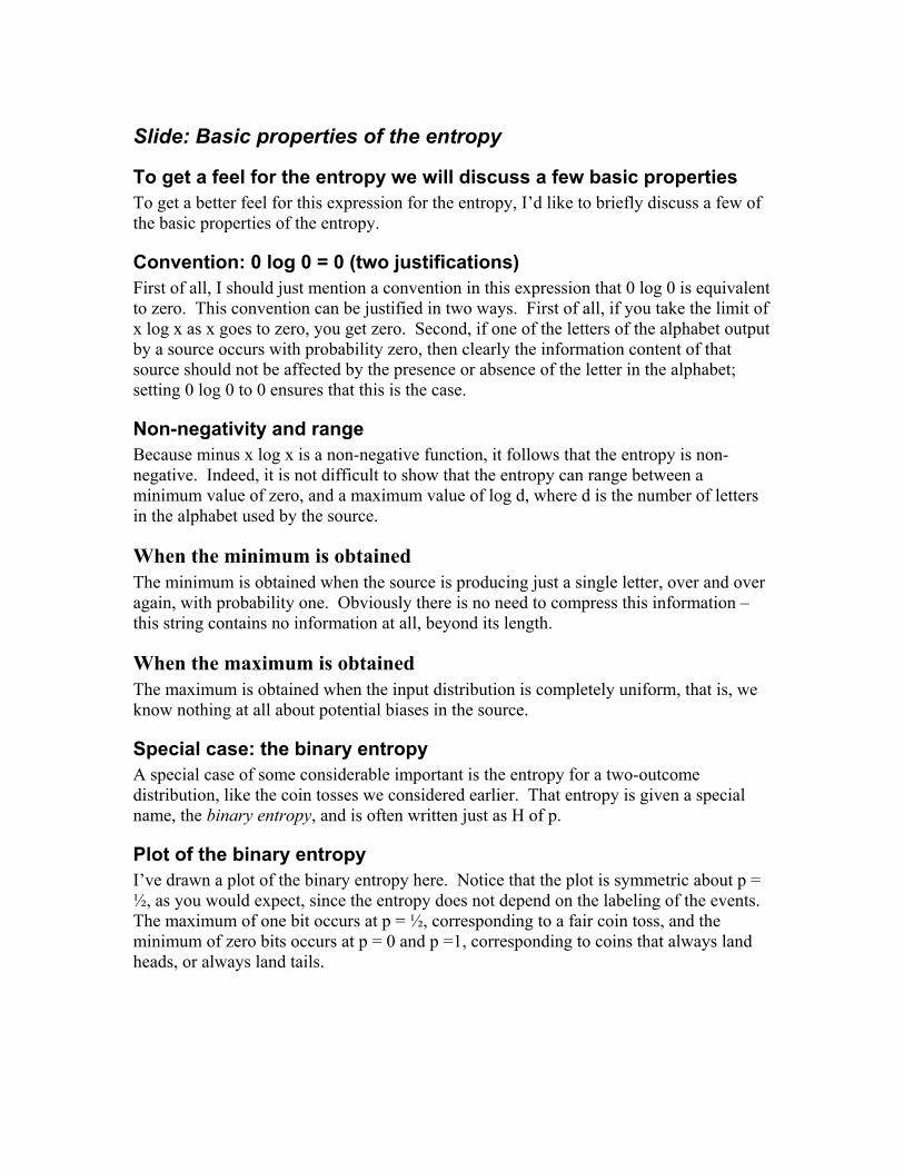
Slide: Basic properties of the entropy

To get a feel for the entropy we will discuss a few basic properties To get a better feel for this expression for the entropy, I’d like to briefly discuss a few of the basic properties of the entropy.

Convention: 0 log 0 = 0 (two justifications) First of all, I should just mention a convention in this expression that 0 log 0 is equivalent to zero. This convention can be justified in two ways. First of all, if you take the limit of x log x as x goes to zero, you get zero. Second, if one of the letters of the alphabet output by a source occurs with probability zero, then clearly the information content of that source should not be affected by the presence or absence of the letter in the alphabet; setting 0 log 0 to 0 ensures that this is the case.

Non-negativity and range Because minus x log x is a non-negative function, it follows that the entropy is non-negative. Indeed, it is not difficult to show that the entropy can range between a minimum value of zero, and a maximum value of log d, where d is the number of letters in the alphabet used by the source.

When the minimum is obtained The minimum is obtained when the source is producing just a single letter, over and over again, with probability one. Obviously there is no need to compress this information – this string contains no information at all, beyond its length.

When the maximum is obtained The maximum is obtained when the input distribution is completely uniform, that is, we know nothing at all about potential biases in the source.

Special case: the binary entropy A special case of some considerable important is the entropy for a two-outcome distribution, like the coin tosses we considered earlier. That entropy is given a special name, the binary entropy, and is often written just as H of p.

Plot of the binary entropy I’ve drawn a plot of the binary entropy here. Notice that the plot is symmetric about p = ½, as you would expect, since the entropy does not depend on the labeling of the events. The maximum of one bit occurs at p = ½, corresponding to a fair coin toss, and the minimum of zero bits occurs at p = 0 and p =1, corresponding to coins that always land heads, or always land tails.

Slide: Why’s it called entropy, anyway?

Connect to the people who’ve done statistical mechanics Some of you who have done thermodynamics and statistical mechanics might be wondering why this quantity is called entropy. After all, isn’t entropy meant to be a measure of disorder in physical systems, not a measure of how much information is being produced by an information source?

Partial answer: it has the same form A partial answer to this question is that, actually, there’s a close mathematical correspondence for the formula for the entropy that Shannon gave, and the usual formula given in thermodynamics textbooks, based on Ludwig Boltzmann’s magnificent formulation of statistical mechanics.

Even so, isn’t it a bad idea to mix the two names up? Even so, you might ask, isn’t it a bad idea to mix the two names up, to avoid confusion?

Shannon thought so too Well, according to the American Heritage Book of English Usage, Shannon was initially worried about this too. But he gave up on this worry after the mathematician John von Neumann advised him to call it entropy, since “no one knows what entropy is, so in the debate you’ll always have the advantage.”

Slide: What else can be done with the Shannon entropy?

What we’ve done We’ve taken a look at the basic properties of the Shannon entropy, and at how it arises from an operational question about the ability to do data compression.

What else can be done with the Shannon entropy? What else can be done with the Shannon entropy?

Recall my claim from earlier in the week Recall my claim from earlier in the week. I outlined a program for doing information science that I called the “fundamental program of information science”. This program had four steps: to identify a physical resource, to identify an information processing task, and to identify a success criterion, and then to ask “How much of 1 do I need to do 2, while satisfying 3?”. My claim was that by following this program, and starting with simple questions about information processing, we would be led to develop notions, like the Shannon entropy, which would be key notions in developing an understanding of more complex information processing tasks.

The context there: quantum The context of my claim earlier in the week was that of complex quantum system, and an upward spiral to the understanding of more and more complex quantum processes.

My claim: this is also true classically My claim is that this is also true classically.

Slide: What else can be done with the Shannon entropy?

How we start In particular, we have started from a relatively simple information-processing task, that of data compression. By following the four step “fundamental program of information science” that I outlined on Monday, we are led to the notion of the Shannon entropy.

What we do next Inspired by our success, we begin to ask more complex question about information, and are able to bootstrap ourselves up to the understanding of more complex processes, making use of deep notions like the Shannon entropy that are discovered along the way.

Give my partial list: noisy channels, crypto, gambling, networks For example, our understanding of the Shannon entropy proved critical to developing an understanding of the problem of doing reliable communication over a noisy channel. Further related areas include cryptography, gambling, and networks of communication channels. In each case, by starting with the simple questions, and just follow the

fundamental program of information science I outlined earlier in the week, and gradually building up an understanding of more complex systems.

Finish the list: , thermo, quantum information, and who knows what else Finally, the concept of the Shannon entropy has even led to new insights into areas that we traditionally think of as being part of physics, like thermodynamics, and even quantum information science, and who knows what else.

Slide: Reliable communication in the presence of noise

What we’re going to do now I’d like to quickly outline just one of these more advanced topics now, before proceeding to discuss quantum entropy. The topic I’m going to discuss is doing communication reliably in the presence of noise.

The scenario The scenario that I’d like you all to imagine is that Alice is trying to send Bob some information over a classical channel.

Presence of noise Unfortunately, that channel is affected by the presence of noise that makes the communication unreliable.

Example: the binary symmetric channel A model of the way such noise acts is provided by the so-called binary symmetric channel. If a bit is input to the binary symmetric channel, then that bit is sent through correctly with probability 1-p, and flipped to the incorrect value with probability p.

Slide: General model of a noisy channel

More general model More generally, we can model the relationship between the input, x, to the channel, and the output, y, by a conditional probability distribution. That is, a list of the probabilities of obtaining the output y, given that the input x was sent.

Example of the binary symmetric channel For example, for the binary symmetric channel, the probability of getting output zero, given the input zero, is one minus p, while the probability of getting output one, given the input zero, is p. Similarly, the probability of getting the output zero given the input one is p, while the probability of getting output one given the input one is one minus p.

Slide: Reliable communication in the presence of noise

Point out that it is possible to communicate reliably even in the presence of such noise Rather remarkably, it turns out that it is possible for Alice to reliably communicate information to Bob, even in the presence of such noise.

Alice’s message Imagine that Alice has a message, M, in her possession that she wishes to send to Bob.

Why she can’t send the message directly Alice can’t send the message directly to Bob, since if she does some parts of the message will inevitably be lost, due to the effect of noise.

Alice’s encoding What she can do instead is encode her message in a longer message, M’, and then transmit that encoded message through the noisy communications channel. This might take many uses of the channel.

Idea that redundancy in the message will enable Bob to decode Bob will receive a corrupted message M’’. However, if Alice has encoded her message in just the right way, the hope is that it will be possible for Bob to decode the corrupted message, and recover the original message, M.

Example: the repetition code As an example of how encoding and decoding might work, imagine the channel is the binary symmetric channel I mentioned on the previous viewgraph. One way for Alice to encode the bits in the message she wants to send is using a so-called “repetition code”. For example, she might encode a zero as three zeroes, and a one as three ones.

How Bob decodes After sending through the channel, Bob decodes the message simply by taking a majority vote: if he gets two or three zeroes, he concludes that Alice was most likely trying to send a zero, and if he gets two or three ones, he concludes that Alice was most likely trying to send a one. In this way they can increase the reliability of their communication, at the cost of having to make their messages somewhat longer.

The question Shannon asked Motivated by this idea, Shannon asked what the fundamental limits were to doing this task. That is, he asked how many uses of the channel – the physical resource - are required to send Alice’s information to Bob – the information processing task – with probability of success approaching one – the criterion for success.

Definition of the channel capacity That is, Shannon asked what the capacity of a noisy channel is, defined to be the maximal number of bits that can be reliably transmitted uses multiple uses of the channel, divided by the number of uses of the channel. Notice that we allow multiple uses of the channel here – this is an asymptotic definition, with long messages and many uses of the channel allowed.

Draw people’s attention to the amazingly complicated nature of the definition This is an amazingly complicated definition, and it is a remarkable fact that Shannon was able to actually come up with a simple formula for the capacity.

Mutual information: motivation To do this, he introduced a concept related to the entropy, known as the mutual information. To understand the mutual information, imagine that random variable, X, is used as input to the noisy channel, which results in an output, Y. The concept of mutual information is intended to capture the notion of what information X and Y have in common. That is, in some sense it quantifies what someone could infer about the identity of X, given that they only know Y.

Mutual information: definition Let me write down the conventional definition for mutual information, and then I’ll tell you a story to help motivate why it’s defined that way. The definition is that the mutual information between X and Y is given by the entropy associated with the probability distribution for X, plus the entropy associated with the probability distribution for Y, minus the entropy associated with the joint probability distribution for X and Y.

Mutual information: Why’s it defined that way? Why is mutual information defined this way? One way of understanding this is to imagine that you have two books of short stories in your hands. However, the two books have a short story in common. Thus, you’d expect that the total information contained in the two books is equal to the sum of the information content of the two books, minus the common information content, which was double counted in the sum. Rearranging this gives the definition for mutual information that I just made.

Comment on the danger of taking this at face value Of course, this isn’t meant to be a rigorous justification for this definition; it’s simply a heuristic argument for why the mutual information could reasonably be defined this way.

doing this. That is, he asked whe

Slide: Worked exercise The worked exercise for this lecture is as follows. Open problems Overview of other applications of the Shannon entropy: Stress first of all that there are many other applications. Give an overview of those: noisy channel coding, control theory, networked information theory, gambling, cryptography. In more detail, explain the connection to noisy channel coding, and explain Shannon’s noisy channel coding theorem. Explain mutual information and what it means: high mutual information means that we can recover the original material. Notion of a quantum information source: Describe a possible way of defining such a source. Description of a source by a density matrix. Problem: how can we quantify the information of a quantum information source? Solution: the von Neumann entropy. Explain the connection to Shannon entropy. Examples: Give the example of two different pure states, say |0> and |0>+|1>. Explain that pure states always have zero entropy. Exercise: Show that the entropy of the completely mixed state I/2 is 1. Quantum data compression: Explain the basic idea. Fidelity criterion: Explain what it means to send information reliably, using the standard average fidelity criterion. Statement of the quantum data compression theorem: Give the statement, explaining each step in detail. Explain how quantum data compression works for a simple example: Do the general case of a qubit. Then give the example of a mixture of |0> and |0>+|1>. Open problem: Determining the maximal rate at which information can be transmitted through a quantum channel. Maybe prove Holevo’s theorem?

Lecture 7: Entanglement

Slide: What is being plotted? To start off the next part of my talk, I’d like to challenge each of you to guess what is being plotted here. Do I have any takers?

Slide: Answer

State the answer The answer is that it’s the number of papers with the term “quantum entanglement” in the title or abstract.

Assert that there are two items of note There are two items of note on this picture.

First: the first paper First is this very first paper, which appeared in 1990.

Who wrote it, and where It was a paper by David Mermin that appeared in Physical Review Letters.

Second: the upward slope The second is this amazing upward slope in the number of papers about entanglement, which started to become visible in 1997.

Question: What caused this? What happened to cause this?

Answer: notion of a theory of entanglement Well, of course, nobody knows, but what I think occurred was that several different insights into the nature of quantum entanglement gradually began to coalesce into a feeling that there ought to be a theory of entanglement developed.

Slogan: “entanglement is a physical resource”, and who publicised it This feeling was captured in the slogan “entanglement is a physical resource”, which was much publicised in a beautiful paper by Bennett, DiVincenzo, Smolin and Wootters, which appeared at the end of 1996.

Slide: Overview

Three-fold goals The goals of this lecture are threefold.

1: Why we regard entanglement as a fundamental physical resource? First, I want to explain why we regard entanglement as a fundamental physical resource, like energy or mass.

2: How to quantify entanglement? Second, I want to explain how we can quantify entanglement.

3: What insights this gives us, into quantum information processing, and physics in general Finally, I will explain how the quantitative theory of entanglement can be used to gain insight into processes of quantum information processing, using the example of quantum teleportation, and how it can also be used to gain insight into more traditional areas of physics, with an example drawn from condensed-matter physics.

Slide: Entanglement revisited Recall that entanglement involves two or more separated parties, (picture) who, for convenience, I’ll call Alice and Bob, although of course, any labels will do.

Scenario To remind you of what entanglement is, imagine that Alice and Bob each have possession of a qubit, and that the joint state of the two qubits is zero zero plus one one over the square root of two.

Property: psi \neq a \otimes b Recall that this state has the remarkable property that it cannot be written as a product of states of Alice’s system alone with Bob’s system alone.

Conclusion: state cannot be understood in terms of its components, but rather is a single, indivisible entity Thus, in some sense, this quantum system cannot be understood in terms of its components, but rather must be understood as a single, indivisible entity.

Schroedinger’s comment Erwin Schroedinger, who first explicitly pointed this property of entanglement out, was so impressed by it that he commented that he would not call entanglement one, but rather the characteristic trait of quantum mechanics, the one that enforces its entire departure from classical lines of thought.

Slide: Entanglement and classicality

State the facts For a long time little work was done on the study of entanglement, until, in the 1960s, John Bell put teeth into Schroedinger’s statement by showing that no locally realistic, that is, classical, theory of the world can explain entanglement. Bell’s ideas were later confirmed experimentally by many groups, most notably by Aspect’s 1982 experiment.

See Peres for an account of these ideas I won’t go into any detail about exactly what Bell showed and Aspect confirmed, however, it’s an absolutely fascinating story, that is beautifully explained in Asher Peres’ book “Quantum theory: concepts and methods”, which I highly recommend as further reading.

Slide: Using entanglement to do stuff

What happened in the 1980s and 1990s In the 1980s and, especially, the 1990s, we discovered that quantum entanglement is actual a useful enabler of tasks such as superdense coding, entanglement-based quantum cryptography, quantum teleportation, and quantum computation.

What we learn What we learn from these and many other examples that have been found since is that entanglement is a useful resource that can be used to accomplish tasks that would otherwise be difficult or impossible.

What can we gain by throwing some entanglement into the problem? In general, then, given any information-processing task, we can always ask ourselves, “what could I gain by throwing some entanglement into the problem?”

Slide: Representation independence of entanglement

State the property A further important property of entanglement is that it has properties that are independent of its particular physical representation.

Introduce the analogy To understand this property, consider an analogy with energy.

Many forms of energy, and unifying principles governing it Energy can be given to us in many different forms, for example, as both solar and electrical energy. However, despite these apparently different forms, energy in any form must obey some fundamental principles, the laws of thermodynamics.

Similarity to entanglement In a similar way, entanglement may given to us in many different forms. The particular entangled state, zero zero plus one one over root two, may be given to us in many different physical forms, including as the spin of a pair of electrons, the polarization of a pair of photons, and so on. Each of these different forms is essentially equivalent, in the sense that they can be utilized to do the same sorts of tasks.

Example: all these forms enable teleportation For example, the rules of quantum mechanics tell us that all of these different forms of entanglement can be used to teleport a qubit from one location to another. In this sense, entanglement therefore has properties that are representation independent, in a similar sense to the representation independence of energy.

Slide: Qualitative equivalence of different entangled states

State the property for energy Energy has a further interesting property, namely, that energy in different forms is qualitatively equivalent, in the sense that even a very small amount of energy can be used to do the same thing as a very large amount of energy, provided enough units of the small amount are available. That is, there is a procedure for going back and forth between the two different types.

State the property for entanglement In a similar way, it turns out that different entangled states are essentially equivalent to one another: there is actually a physical procedure that can be used to convert one to the other. For example, we will see later that two copies of this state here is essentially equivalent to three copies of the maximally entangled qubit state! More generally, it turns out to be possible to convert back and forth between different types of entangled states, and I will describe how this is done later in the lecture.

Slide: Summary

Summarize Summarizing, entanglement has properties that are not classical, it is useful physical resource that enables interesting tasks, it has properties that are independent of physical representation, and it turns out that different entangled states are qualitatively equivalent to one another, in the sense that given enough of one it is possible to convert it into the other state.

The question these properties motivate These properties motivate a point of view that maybe entanglement is more than just the property of not being writeable as a product state. Maybe entanglement is deeper, and it is possible to develop a quantitative theory of entangled states. Over the past few years an enormous amount of effort has been devoted to developing such a theory, and that is the subject of the remainder of this lecture.

Slide: What might we get out of such a theory?

Raise the question What might we get out of such a theory of entanglement?

What we get out of thermodynamics Well, in the case of thermodynamics we have a set of principles governing the transport and harnessing of heat and other forms of energy in physical systems.

What we hope to get out of a theory of entanglement In the case of the theory of entanglement we hope to obtain a similarly powerful set of high-level principles governing the creation, dynamics, observation and characterization of entanglement.

Slide: How can we quantify entanglement?

Raise the question How can we hope to begin developing such a quantitative theory of entanglement?

Recall the connection with information Well, recall from earlier in the week that we saw that there is a close connection between entanglement and various information processing-tasks. This was indicated by phenomena such a superdense coding and teleportation, which suggested various relationships between bits, qubits, and entanglement.

What approach we should take These relationships are perhaps not precise enough to be considered rigorous inequalities, but they are suggestive. In particular, they suggest that perhaps the appropriate way of attempting to quantify entanglement is similar to the approach taken to the quantification of information, as I described in yesterday’s lecture on entropy.

Bring in the fundamental question of information science In particular, it suggests that the appropriate way of quantifying entanglement might be to start with the fundamental question of information science.

What we’re going to do now What I’m going to do now is to sketch several different possible ways in which we can use the fundamental question of information science to define a notion of entanglement.

Why this might cause discomfort At various points my presentation might cause some discomfort, for there are some points at which the way in which I use the fundamental question appears ad hoc. There’s a very good reason for this, and that is, that nobody is yet sure what the correct way of defining a measure of entanglement. Instead, we have various candidate measures, and it is by no means clear which is the best. This is all very much a work in progress.

Slide: Distillable entanglement

Inspired by teleportation With that caveat in mind, let’s begin exploring various approaches we can take. The first approach is based on the idea of teleportation. One way of describing the essence of teleportation is that it is a protocol that uses shared entanglement and classical communication to accomplish the transmission of qubits. Teleportation utilizes Bell state entanglement to accomplish this, however we will ask whether a similar task can be accomplished using a more general entangled state.

Physical resource The physical resource for this problem is going to be a large number of copies of the state, psi, whose entanglement we are attempting to quantify. We will also allow unlimited classical communication, and the ability for Alice and Bob to perform arbitrary local operations on their systems, including measurements and so on.

Task and criterion for success The information processing task is for Alice to use these resources to transmit qubits to Bob, with the fidelity of the transmission approaching one. To make the analysis easier we assume that we’re working in the asymptotic limit, where large numbers of copies of psi are available, and the goal is to transmit large numbers of qubits.

The fundamental question The fundamental question, then, is how many copies of psi are required to reliably communicate qubits from Alice to Bob.

Quantification We can quantify this number by defining the entanglement present in psi to be the ratio of the maximal number of qubits that can be communicated, per copy of psi that was initially shared.

Technical caveats Note, incidentally, that I have been rather vague about certain features. In particular, there is an implicit asymptotic limit being taken, and certain details about the reliability criterion that I am ignoring. Filling those details in is not especially difficult, although it does need to be done. My goal today is to present the broad picture of how entanglement is defined; for the rigorous details, you will need to look into one of the may excellent review articles about this material.

Why is this called distillable entanglement? Now this does seem like a reasonable way of quantifying entanglement – after all, it quantifies how well our copy of psi enables an information processing task – but it might seem a little strange that I have called this the distillable entanglement.

What we’re going to do To understand this I’m going to reformulate this entanglement measure in terms of a different information processing task. Instead of Alice trying to send qubits to Bob, I’m going to ask that they do something else which is on the face of it very different. Imagine that instead the goal were for Alice and Bob to use their physical resources to try and set up shared Bell states.

Summarize That is, Alice and Bob would try to go from their shared copies of psi to shared Bell states. This process is called “distillation”, and I’ll give an example to illustrate how it works in a moment.

How the question is reformulated However, accepting for the moment that this is possible, it’s not difficult to see that this is completely equivalent to the task I previously considered. To see this, note that Representation-independence and qualitative equivalence: Maybe I should just talk about representation independence and the way that motivates quantification of entanglement. Explain the point behind quantifying entanglement: Give the colour diagram. Big picture: We want to quantify entanglement in order to understand other tasks. Give the thermodynamic analogy. Maybe give the analogy of heat flowing around a building; what we’d like to do is look at entanglement flowing through a system. Can this be used to analyse problems? Explain how we quantify entanglement: Use the mass analogy to introduce the definition. Also stress that what we are doing is following Schumacher’s program. Explain why it is that the entropy is the answer: First, explain how to do the dilution step, via Schumacher compression. Not sure how to do the concentration step. Example: Analysis of distributed computational problems: Give the general context: evaluation of a function by two parties. Stress the connection to Schumacher, again. Explain the log-rank lower bound, following my lecture at the Gold Coast last year. Example: analysis of approximate teleportation. Just follow what I’ve already done in the ITP lecture.

Overview of current work: Multi-party entanglement. Mixed state entanglement. Attempts to connect entanglement to other work. Examples of three-party entanglement: Give the GHZ state. Explain the W-state. A problem with all this is that it is very abstract. Can it be made more concrete? Do I want to explain the significance of LOCC in terms of equivalence classes of different channels? I think the main point is to try to give some idea of the direction of current research.

Lecture 8: Quantum Communication Overview: Idea is to discuss the properties of quantum communication channels. In particular, we wish to discuss the different types of information that can be transmitted over such channels. Reminder: what is a quantum communication channel. Give the example of the depolarizing, bit flip and dephasing channels. Basic idea, then, is to determine the fundamental properties of such channels. In particular, we wish to enable what information processing tasks such channels enable us to do. It turns out that a simple set of numbers can be used to summarize that. Example: in the classical case, all that matters is the capacity of a channel. If we know that number, then we know how much information the channel can transmit. In quantum mechanics there are more types of information, so there are more questions to answer; it is not so clear what the relationships will be. Different types of physical resource that can be transmitted over a channel: Examples of entanglement, classical information, or quantum states. Might there be other types of physical resource? Simplest type of communication problem: Imagine that Bob wants to identify a quantum state given to him by Alice. Then the mutual information is bounded. Explain the proof of the Holevo bound. Explain why the Holevo bound limits the amount of information in a qubit to just a single bit. More generally: Explain the HSW formula for information transmission over a quantum channel. Explain the open problems associated. Capacity of a channel for entanglement, or for quantum information: Give the definition, and give some simple examples. Point out that giving a general formula is still an open problem. Maybe conclude by noting the strange phenomenon of the two-way capacity being non-zero. Perhaps I could talk about quantum cryptography here.

Potentially a major theme for the entire week might be the idea of understanding what a physical resource is. What do we mean when we talk about “physical resources”? The broad idea underlying the work on quantum communication channels is to understand the different sorts of information transmission that can be done in quantum mechanics. What would be a good time to discuss the question: what is a physical resource? The answer to both those questions is not entirely clear. Probably a good spot is in the lecture about entanglement. I’m not entirely clear on the answer to the question, myself. We can always try to develop a quantitative theory for the description of a physical resource: the question is, do we want to?