Embed Size (px)
Citation preview
Lecture Notes in Mathematics 1861Editors:J.--M. Morel, CachanF. Takens, GroningenB. Teissier, Paris
Subseries:Fondazione C.I.M.E., FirenzeAdviser: Pietro Zecca
Giancarlo BenettinJacques HenrardSergei Kuksin
Hamiltonian DynamicsTheory and ApplicationsLectures given at theC.I.M.E.-E.M.S. Summer Schoolheld in Cetraro, Italy,July 1--10, 1999
Editor: Antonio Giorgilli
123
Editors and Authors
Giancarlo BenettinDipartimento di Matematica Pura e ApplicataUniversita di PadovaVia G. Belzoni 735131 Padova, Italy
e-mail: [email protected]
Antonio GiorgilliDipartimento di Matematica e ApplicazioniUniversita degli Studi di Milano BicoccaVia Bicocca degli Arcimboldi 820126 Milano, Italy
e-mail: [email protected]
Jacques HenrardDepartement de MathematiquesFUNDP 8Rempart de la Vierge5000 Namur, Belgium
e-mail: [email protected]
Sergei KuksinDepartment of MathematicsHeriot-Watt UniversityEdinburghEH14 4AS, United KingdomandSteklov Institute of Mathematics8 Gubkina St.111966 Moscow, Russia
e-mail: [email protected]
Library of Congress Control Number: 2004116724Mathematics Subject Classification (2000): 70H07, 70H14, 37K55, 35Q53, 70H11, 70E17
ISSN 0075-8434ISBN 3-540-24064-0 Springer Berlin Heidelberg New YorkDOI: 10.1007/b104338
This work is subject to copyright. All rights are reserved, whether the whole or part of the material isconcerned, specif ically the rights of translation, reprinting, reuse of illustrations, recitation, broadcasting,reproduction on microf ilm or in any other way, and storage in data banks. Duplication of this publicationor parts thereof is permitted only under the provisions of the German Copyright Law of September 9, 1965,in its current version, and permission for use must always be obtained from Springer. Violations are liablefor prosecution under the German Copyright Law.
Springer is a part of Springer Science + Business Mediahttp://www.springeronline.comc© Springer-Verlag Berlin Heidelberg 2005
Printed in Germany
The use of general descriptive names, registered names, trademarks, etc. in this publication does not imply,even in the absence of a specif ic statement, that such names are exempt from the relevant protective lawsand regulations and therefore free for general use.
Typesetting: Camera-ready TEX output by the authors
41/3142/ du - 543210 - Printed on acid-free paper
Preface
“ Nous sommes donc conduit a nous proposer le probleme suivant:Etudier les equations canoniques
dxidt
=∂F
∂yi,
dyidt
= − ∂F∂xi
en supposant que la function F peut se developper suivant lespuissances d’un parametre tres petit µ de la maniere suivante:
F = F0 + µF1 + µ2F2 + . . . ,
en supposant de plus que F0 ne depend que des x et est independentdes y; et que F1, F2, . . . sont des fonctions periodiques de periode2π par rapport aux y. ”
This is all of the contents of §13 in the first volume of the celebrated treatiseLes methodes nouvelles de la mecanique celeste of Poincare, published in 1892.
In more usual notations and words, the problem is to investigate the dy-namics of a canonical system of differential equations with Hamiltonian
(1) H(p, q, ε) = H0(p) + εH1(p, q) + ε2H2(p, q) + . . . ,
where p ≡ (p1, . . . , pn) ∈ G ⊂ Rn are action variables in the open set G,q ≡ (q1, . . . , qn) ∈ Tn are angle variables, and ε is a small parameter.
The lectures by Giancarlo Benettin, Jacques Henrard and Sergej Kuksinpublished in the present book address some of the many questions that arehidden behind the simple sentence above.
1. A Classical Problem
It is well known that the investigations of Poincare were motivated by a clas-sical problem: the stability of the Solar System. The three volumes of the
VI Preface
Methodes Nouvelles had been preceded by the memoir Sur le probleme destrois corps et les equations de la dynamique; memoire couronne du prix deS. M. le Roi Oscar II le 21 janvier 1889.
It may be interesting to recall the subject of the investigation, as statedin the announcement of the competition for King Oscar’s prize:
“ A system being given of a number whatever of particles attractingone another mutually according to Newton’s law, it is proposed,on the assumption that there never takes place an impact of twoparticles to expand the coordinates of each particle in a series pro-ceeding according to some known functions of time and converginguniformly for any space of time. ”
In the announcement it is also mentioned that the question was suggestedby a claim made by Lejeune–Dirichlet in a letter to a friend that he hadbeen able to demonstrate the stability of the solar system by integrating thedifferential equations of Mechanics. However, Dirichlet died shortly after, andno reference to his method was actually found in his notes.
As a matter of fact, in his memoir and in the Methodes Nouvelles Poincareseems to end up with different conclusions. Just to mention a few results of hiswork, let me recall the theorem on generic non–existence of first integrals, therecurrence theorem, the divergence of classical perturbation series as a typicalfact, the discovery of asymptotic solutions and the existence of homoclinicpoints.
Needless to say, the work of Poincare represents the starting point of mostof the research on dynamical systems in the XX–th century. It has also beensaid that the memoir on the problem of three bodies is “the first textbookin the qualitative theory of dynamical systems”, perhaps forgetting that thequalitative study of dynamics had been undertaken by Poincare in a Memoiresur les courbes definies par une equation differentielle, published in 1882.
2. KAM Theory
Let me recall a few known facts about the system (1). For ε = 0 the Hamilto-nian possesses n first integrals p1, . . . , pn that are independent, and the orbitslie on invariant tori carrying periodic or quasi–periodic motions with frequen-cies ω1(p), . . . , ωn(p), where ωj(p) = ∂H0
∂pj. This is the unperturbed dynamics.
For ε = 0 this plain behaviour is destroyed, and the problem is to understandhow the dynamics actually changes.
The classical methods of perturbation theory, as started by Lagrange andLaplace, may be resumed by saying that one tries to prove that for ε = 0the system (1) is still integrable. However, this program encountered majordifficulties due to the appearance in the expansions of the so called secular
Preface VII
terms, generated by resonances among the frequencies. Thus the problembecome that of writing solutions valid for all times, possibly expanded inpower series of the parameter ε. By the way, the role played by resonances isindeed at the basis of the non–integrability in classical sense of the perturbedsystem, as stated by Poincare.
A relevant step in removing secular terms was made by Lindstedt in 1882.The underlying idea of Lindstedt’s method is to look for a single solutionwhich is characterized by fixed frequencies, λ1, . . . , λn say, and which is closeto the unperturbed torus with the same frequencies. This allowed him toproduce series expansions free from secular terms, but he did not solve theproblem of the presence of small denominators, i.e., denominators of the form〈k, λ〉 where 0 = k ∈ Zn. Even assuming that these quantities do not vanish(i.e., excluding resonances) they may become arbitrarily small, thus makingthe convergence of the series questionable.
In tome II, chap. XIII, § 148–149 of the Methodes Nouvelles Poincaredevoted several pages to the discussion of the convergence of the series ofLindstedt. However, the arguments of Poincare did not allow him to reach adefinite conclusion:
“ . . . les series ne pourraient–elles pas, par example, converger quand. . . le rapport n1/n2 soit incommensurable, et que son carre soit aucontraire commensurable (ou quand le rapport n1/n2 est assujettia une autre condition analogue a celle que je viens d’ enoncer unpeu au hasard)?
Les raisonnements de ce chapitre ne me permettent pasd’ affirmer que ce fait ne se presentera pas. Tout ce qu’ il m’estpermis de dire, c’est qu’ il est fort invraisemblable. ”
Here, n1, n2 are the frequencies, that we have denoted by λ1, λ2.The problem of the convergence was settled in an indirect way 60 years
later by Kolmogorov, when he announced his celebrated theorem. In brief, ifthe perturbation is small enough, then most (in measure theoretic sense) ofthe unperturbed solutions survive, being only slightly deformed. The survivinginvariant tori are characterized by some strong non–resonance conditions, thatin Kolmogorov’s note was identified with the so called diophantine condition,namely
∣∣〈k, λ〉
∣∣ ≥ γ|k|−τ for some γ > 0, τ > n − 1 and for all non–zero
k ∈ Zn. This includes the case of the frequencies chosen “un peu au hasard”by Poincare. It is often said that Kolmogorov announced his theorem withoutpublishing the proof; as a matter of fact, his short communication contains asketch of the proof where all critical elements are clearly pointed out. Detailedproofs were published later by Moser (1962) and Arnold (1963); the theorembecome thus known as KAM theorem.
The argument of Kolmogorov constitutes only an indirect proof of theconvergence of the series of Lindstedt; this has been pointed out by Moser in1967. For, the proof invented by Kolmogorov is based on an infinite sequence of
VIII Preface
canonical transformations that give the Hamiltonian the appropriate normalform
H(p, q) = 〈λ, p〉+R(p, q) ,
where R(p, q) is at least quadratic in the action variables p. Such a Hamil-tonian possesses the invariant torus p = 0 carrying quasi–periodic motionswith frequencies λ. This implies that the series of Lindstedt must converge,since they give precisely the form of the solution lying on the invariant torus.However, Moser failed to obtain a direct proof based, e.g., on Cauchy’s clas-sical method of majorants applied to Lindstedt’s expansions in powers of ε.As discovered by Eliasson, this is due to the presence in Lindstedt’s classicalseries of terms that grow too fast, due precisely to the small denominators,but are cancelled out by internal compensations (this was written in a reportof 1988, but was published only in 1996). Explicit constructive algorithms tak-ing compensations into account have been recently produced by Gallavotti,Chierchia, Falcolini, Gentile and Mastropietro.
In recent years, the perturbation methods for Hamiltonian systems, and inparticular the KAM theory, has been extended to the case of PDE’s equations.The lectures of Kuksin included in this volume constitute a plain and completepresentation of these recent theories.
3. Adiabatic Invariants
The theory of adiabatic invariants is related to the study of the dynamics ofsystems with slowly varying parameters. That is, the Hamiltonian H(q, p ;λ)depends on a parameter λ = εt, with ε small. The typical simple exampleis a pendulum the length of which is subjected to a very slow change – e.g.,a periodic change with a period much longer than the proper period of thependulum. The main concern is the search for quantities that remain closeto constants during the evolution of the system, at least for reasonably longtime intervals. This is a classical problem that has received much attention atthe beginning of the the XX–th century, when the quantities to be consideredwere identified with the actions of the system.
The usefulness of the action variables has been particularly emphasizedin the book of Max Born The Mechanics of the Atom, published in 1927. Inthat book the use of action variables in quantum theory is widely discussed.However, it should be remarked that most of the book is actually devoted toHamiltonian dynamics and perturbation methods. In this connection it maybe interesting to quote the first few sentences of the preface to the germanedition of the book:
“ The title “Atomic Mechanics” given to these lectures . . . was chosento correspond to the designation “Celestial Mechanics”. As thelatter term covers that branch of theoretical astronomy which deals
Preface IX
with with the calculation of the orbits of celestial bodies accordingto mechanical laws, so the phrase “Atomic Mechanics” is chosento signify that the facts of atomic physics are to be treated herewith special reference to the underlying mechanical principles; anattempt is made, in other words, at a deductive treatment of atomictheory. ”
The theory of adiabatic invariants is discussed in this volume in the lecturesof J. Henrard. The discussion includes in particular some recent developmentsthat deal not just with the slow evolution of the actions, but also with thechanges induced on them when the orbit crosses some critical regions. Makingreference to the model of the pendulum, a typical case is the crossing of theseparatrix. Among the interesting phenomena investigated with this methodone will find, e.g., the capture of the orbit in a resonant regions and thesweeping of resonances in the Solar System.
4. Long–Time Stability and Nekhoroshev’s Theory
Although the theorem of Kolmogorov has been often indicated as the solu-tion of the problem of stability of the Solar System, during the last 50 yearsit became more and more evident that it is not so. An immediate remarkis that the theorem assures the persistence of a set of invariant tori withrelative measure tending to one when the perturbation parameter ε goes tozero, but the complement of the invariant tori is open and dense, thus mak-ing the actual application of the theorem to a physical system doubtful, dueto the indeterminacy of the initial conditions. Only the case of a system oftwo degrees of freedom can be dealt with this way, since the invariant toricreate separated gaps on the invariant surface of constant energy. Moreover,the threshold for the applicability of the theorem, i.e., the actual value of εbelow which the theorem applies, could be unrealistic, unless one considersvery localized situations. Although there are no general definite proofs in thissense, many numerical calculations made independently by, e.g., A. Milani,J. Wisdom and J. Laskar, show that at least the motion of the minor planetslooks far from being a quasi–periodic one.
Thus, the problem of stability requires further investigation. In this re-spect, a way out may be found by proving that some relevant quantities,e.g., the actions of the system, remain close to their initial value for a longtime; this could lead to a sort of “effective stability” that may be enough forphysical application. In more precise terms, one could look for an estimate∣∣p(t) − p(0)
∣∣ = O(εa) for all times |t| < T (ε), were a is some number in the
interval (0, 1) (e.g., a = 1/2 or a = 1/n), and T (ε) is a “large” time, in somesense to be made precise.
The request above may be meaningful if we take into consideration somecharacteristics of the dynamical system that is (more or less accurately) de-
X Preface
scribed by our equations. In this case the quest for a “large” time should beinterpreted as large with respect to some characteristic time of the physicalsystem, or comparable with the lifetime of it. For instance, for the nowadaysaccelerators a characteristic time is the period of revolution of a particle ofthe beam and the typical lifetime of the beam during an experiment maybe a few days, which may correspond to some 1010 revolutions; for the solarsystem the lifetime is the estimated age of the universe, which correspondsto some 1010 revolutions of Jupiter; for a galaxy, we should consider that thestars may perform a few hundred revolutions during a time as long as the ageof the universe, which means that a galaxy does not really need to be muchstable in order to exist.
From a mathematical viewpoint the word “large” is more difficult to ex-plain, since there is no typical lifetime associated to a differential equation.Hence, in order to give the word “stability” a meaning in the sense above itis essential to consider the dependence of the time T on ε. In this respect thecontinuity with respect to initial data does not help too much. For instance,if we consider the trivial example of the equilibrium point of the differentialequation x = x one will immediately see that if x(0) = x0 > 0 is the initialpoint, then we have x(t) > 2x0 for t > T = ln 2 no matter how small is x0;hence T may hardly be considered to be “large”, since it remains constantas x0 decreases to 0. Conversely, if for a particular system we could prove,e.g., that T (ε) = O(1/ε) then our result would perhaps be meaningful; this isindeed the typical goal of the theory of adiabatic invariants.
Stronger forms of stability may be found by proving, e.g., that T (ε) ∼1/εr for some r > 1; this is indeed the theory of complete stability due toBirkhoff. As a matter of fact, the methods of perturbation theory allow usto prove more: in the inequality above one may actually choose r dependingon ε, and increasing when ε → 0. In this case one obtains the so calledexponential stability, stating that T (ε) ∼ exp(1/εb) for some b. Such a strongresult was first stated by Moser (1955) and Littlewood (1959) in particularcases. A complete theory in this direction was developed by Nekhoroshev, andpublished in 1978.
The lectures of Benettin in this volume deal with the application of thetheory of Nekhoroshev to some interesting physical systems, including the col-lision of molecules, the classical problem of the rigid body and the triangularLagrangian equilibria of the problem of three bodies.
Acknowledgements
This volume appears with the essential contribution of the Fondazione CIME.The editor wishes to thank in particular A. Cellina, who encouraged him toorganize a school on Hamiltonian systems.
The success of the school has been assured by the high level of the lecturesand by the enthusiasm of the participants. A particular thankfulness is due
Preface XI
to Giancarlo Benettin, Jacques Henrard and Sergej Kuksin, who acceptednot only to profess their excellent lectures, but also to contribute with theirwritings to the preparation of this volume
Milano, March 2004 Antonio GiorgilliProfessor of Mathematical PhysicsDepartment of MathematicsUniversity of Milano Bicocca
CIME’s activity is supported by:
Ministero dell’ Universita Ricerca Scientifica e Tecnologica;Consiglio Nazionale delle Ricerche;E.U. under the Training and Mobility of Researchers Programme.

Contents
Physical Applications of Nekhoroshev Theorem andExponential EstimatesGiancarlo Benettin . . . . . . . . . . . . . . . . . . . . . . . . . . . . . . . . . . . . . . . . . . . . . . . 11 Introduction . . . . . . . . . . . . . . . . . . . . . . . . . . . . . . . . . . . . . . . . . . . . . . . . . . 12 Exponential Estimates . . . . . . . . . . . . . . . . . . . . . . . . . . . . . . . . . . . . . . . . . 53 A Rigorous Version of the JLT Approximation in a Model . . . . . . . . . . 234 An Application of the JLT Approximation . . . . . . . . . . . . . . . . . . . . . . . . 325 The Essentials of Nekhoroshev Theorem . . . . . . . . . . . . . . . . . . . . . . . . . . 396 The Perturbed Euler–Poinsot Rigid Body . . . . . . . . . . . . . . . . . . . . . . . . 497 The Stability of the Lagrangian Equilibrium Points L4 − L5 . . . . . . . . 62References . . . . . . . . . . . . . . . . . . . . . . . . . . . . . . . . . . . . . . . . . . . . . . . . . . . . . . 73
The Adiabatic Invariant Theory and ApplicationsJacques Henrard . . . . . . . . . . . . . . . . . . . . . . . . . . . . . . . . . . . . . . . . . . . . . . . . . 771 Integrable Systems . . . . . . . . . . . . . . . . . . . . . . . . . . . . . . . . . . . . . . . . . . . . 77
1.1 Hamilton-Jacobi Equation . . . . . . . . . . . . . . . . . . . . . . . . . . . . . . . . . . 77Canonical Transformations . . . . . . . . . . . . . . . . . . . . . . . . . . . . . . . . . 77Hamilton-Jacobi Equation . . . . . . . . . . . . . . . . . . . . . . . . . . . . . . . . . . 78
1.2 Integrables Systems . . . . . . . . . . . . . . . . . . . . . . . . . . . . . . . . . . . . . . . . 79Liouville Theorem . . . . . . . . . . . . . . . . . . . . . . . . . . . . . . . . . . . . . . . . . 79Stackel Systems . . . . . . . . . . . . . . . . . . . . . . . . . . . . . . . . . . . . . . . . . . . 80Russian Dolls Systems . . . . . . . . . . . . . . . . . . . . . . . . . . . . . . . . . . . . . 81
1.3 Action-Angle Variables . . . . . . . . . . . . . . . . . . . . . . . . . . . . . . . . . . . . . 82One-Degree of Freedom . . . . . . . . . . . . . . . . . . . . . . . . . . . . . . . . . . . . 82Two Degree of Freedom Separable Systems . . . . . . . . . . . . . . . . . . . 86
2 Classical Adiabatic Theory . . . . . . . . . . . . . . . . . . . . . . . . . . . . . . . . . . . . . 89The Adiabatic Invariant . . . . . . . . . . . . . . . . . . . . . . . . . . . . . . . . . . . . 89Applications . . . . . . . . . . . . . . . . . . . . . . . . . . . . . . . . . . . . . . . . . . . . . . 92The Modulated Harmonic Oscillator . . . . . . . . . . . . . . . . . . . . . . . . . 92The Two Body Problem. . . . . . . . . . . . . . . . . . . . . . . . . . . . . . . . . . . . 93The Pendulum . . . . . . . . . . . . . . . . . . . . . . . . . . . . . . . . . . . . . . . . . . . . 93The Magnetic Bottle . . . . . . . . . . . . . . . . . . . . . . . . . . . . . . . . . . . . . . . 96
XIV Contents
3 Neo-adiabatic Theory . . . . . . . . . . . . . . . . . . . . . . . . . . . . . . . . . . . . . . . . . . 1013.1 Introduction . . . . . . . . . . . . . . . . . . . . . . . . . . . . . . . . . . . . . . . . . . . . . . 1013.2 Neighborhood of an Homoclinic Orbit . . . . . . . . . . . . . . . . . . . . . . . . 1023.3 Close to the Equilibrium . . . . . . . . . . . . . . . . . . . . . . . . . . . . . . . . . . . 1043.4 Along the Homoclinic Orbit . . . . . . . . . . . . . . . . . . . . . . . . . . . . . . . . 1073.5 Traverse from Apex to Apex . . . . . . . . . . . . . . . . . . . . . . . . . . . . . . . . 1093.6 Probability of Capture . . . . . . . . . . . . . . . . . . . . . . . . . . . . . . . . . . . . . 1133.7 Change in the Invariant . . . . . . . . . . . . . . . . . . . . . . . . . . . . . . . . . . . . 1173.8 Applications . . . . . . . . . . . . . . . . . . . . . . . . . . . . . . . . . . . . . . . . . . . . . . 121
The Magnetic Bottle . . . . . . . . . . . . . . . . . . . . . . . . . . . . . . . . . . . . . . . 121Resonance Sweeping in the Solar System . . . . . . . . . . . . . . . . . . . . . 122
4 Slow Chaos . . . . . . . . . . . . . . . . . . . . . . . . . . . . . . . . . . . . . . . . . . . . . . . . . . . 1274.1 Introduction . . . . . . . . . . . . . . . . . . . . . . . . . . . . . . . . . . . . . . . . . . . . . . 1274.2 The Frozen System . . . . . . . . . . . . . . . . . . . . . . . . . . . . . . . . . . . . . . . . 1284.3 The Slowly Varying System . . . . . . . . . . . . . . . . . . . . . . . . . . . . . . . . . 1294.4 Transition Between Domains . . . . . . . . . . . . . . . . . . . . . . . . . . . . . . . . 1304.5 The “MSySM” . . . . . . . . . . . . . . . . . . . . . . . . . . . . . . . . . . . . . . . . . . . . 1334.6 Slow Crossing of the Stochastic Layer . . . . . . . . . . . . . . . . . . . . . . . . 136
References . . . . . . . . . . . . . . . . . . . . . . . . . . . . . . . . . . . . . . . . . . . . . . . . . . . . . . 139
Lectures on Hamiltonian Methods in Nonlinear PDEsSergei Kuksin . . . . . . . . . . . . . . . . . . . . . . . . . . . . . . . . . . . . . . . . . . . . . . . . . . . 1431 Symplectic Hilbert Scales and Hamiltonian Equations . . . . . . . . . . . . . . 143
1.1 Hilbert Scales and Their Morphisms . . . . . . . . . . . . . . . . . . . . . . . . . 1431.2 Symplectic Structures . . . . . . . . . . . . . . . . . . . . . . . . . . . . . . . . . . . . . . 1451.3 Hamiltonian Equations . . . . . . . . . . . . . . . . . . . . . . . . . . . . . . . . . . . . . 1461.4 Quasilinear and Semilinear Equations . . . . . . . . . . . . . . . . . . . . . . . . 147
2 Basic Theorems on Hamiltonian Systems . . . . . . . . . . . . . . . . . . . . . . . . . 1483 Lax-Integrable Equations . . . . . . . . . . . . . . . . . . . . . . . . . . . . . . . . . . . . . . . 150
3.1 General Discussion . . . . . . . . . . . . . . . . . . . . . . . . . . . . . . . . . . . . . . . . 1503.2 Korteweg–de Vries Equation . . . . . . . . . . . . . . . . . . . . . . . . . . . . . . . . 1523.3 Other Examples . . . . . . . . . . . . . . . . . . . . . . . . . . . . . . . . . . . . . . . . . . . 153
4 KAM for PDEs . . . . . . . . . . . . . . . . . . . . . . . . . . . . . . . . . . . . . . . . . . . . . . . 1544.1 Perturbations of Lax-Integrable Equation . . . . . . . . . . . . . . . . . . . . 1544.2 Perturbations of Linear Equations . . . . . . . . . . . . . . . . . . . . . . . . . . . 1554.3 Small Oscillation in Nonlinear PDEs . . . . . . . . . . . . . . . . . . . . . . . . . 155
5 The Non-squeezing Phenomenon and Symplectic Capacity . . . . . . . . . . 1565.1 The Gromov Theorem . . . . . . . . . . . . . . . . . . . . . . . . . . . . . . . . . . . . . 1565.2 Infinite-Dimensional Case . . . . . . . . . . . . . . . . . . . . . . . . . . . . . . . . . . 1565.3 Examples . . . . . . . . . . . . . . . . . . . . . . . . . . . . . . . . . . . . . . . . . . . . . . . . 1595.4 Symplectic Capacity . . . . . . . . . . . . . . . . . . . . . . . . . . . . . . . . . . . . . . . 160
6 The Squeezing Phenomenon . . . . . . . . . . . . . . . . . . . . . . . . . . . . . . . . . . . . 161References . . . . . . . . . . . . . . . . . . . . . . . . . . . . . . . . . . . . . . . . . . . . . . . . . . . . . . 163
Physical Applications of Nekhoroshev Theoremand Exponential Estimates
Giancarlo Benettin
Universita di Padova, Dipartimento di Matematica Pura e Applicata,Via G. Belzoni 7, 35131 Padova, [email protected]
1 Introduction
The purpose of these lectures is to discuss some physical applications of Hamil-tonian perturbation theory. Just to enter the subject, let us consider the usualsituation of a nearly-integrable Hamiltonian system,
H(I, ϕ) = h(I) + εf(I, ϕ) , I = (I1, . . . , In) ∈ B ⊂ Rn
ϕ = (ϕ1, . . . , ϕn) ∈ Tn , (1.1)
B being a ball in Rn. As we shall see, such a framework is often poor and not
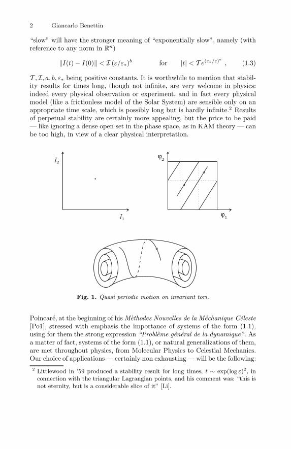
really adequate for some important physical applications, nevertheless it is anatural starting point. For ε = 0 the phase space is decomposed into invarianttori
I
× Tn, see figure 1, on which the flow is linear:
I(t) = Io , ϕ(t) = ϕo + ω(Io)t ,
with ω = ∂h∂I . For ε = 0 one is instead confronted with the nontrivial equations
I = −ε ∂f∂ϕ
(I, ϕ) , ϕ = ω(I) + ε∂f
∂I(I, ϕ) . (1.2)
Different stategies can be used in front of such equations, all of them sharingthe elementary idea of “averaging out” in some way the term ∂f
∂ϕ , to show that,in convenient assumptions, the evolution of the actions (if any) is very slow.In perturbation theory, “slow” means in general that ‖I(t) − I(0)‖ remainssmall, for small ε, at least for t ∼ 1/ε (that is: the evolution is slower than thetrivial a priori estimate following (1.2)). Throughout these lectures, however, Gruppo Nazionale di Fisica Matematica and Istituto Nazionale di Fisica della
Materia
G. Benettin, J. Henrard, and S. Kuksin: LNM 1861, A. Giorgilli (Ed.), pp. 1–76, 2005.c© Springer-Verlag Berlin Heidelberg 2005
2 Giancarlo Benettin
“slow” will have the stronger meaning of “exponentially slow”, namely (withreference to any norm in R
n)
‖I(t)− I(0)‖ < I (ε/ε∗)b for |t| < T e(ε∗/ε)a
, (1.3)
T , I, a, b, ε∗ being positive constants. It is worthwhile to mention that stabil-ity results for times long, though not infinite, are very welcome in physics:indeed every physical observation or experiment, and in fact every physicalmodel (like a frictionless model of the Solar System) are sensible only on anappropriate time scale, which is possibly long but is hardly infinite.2 Resultsof perpetual stability are certainly more appealing, but the price to be paid— like ignoring a dense open set in the phase space, as in KAM theory — canbe too high, in view of a clear physical interpretation.
Fig. 1. Quasi periodic motion on invariant tori.
Poincare, at the beginning of his Methodes Nouvelles de la Mechanique Celeste[Po1], stressed with emphasis the importance of systems of the form (1.1),using for them the strong expression “Probleme general de la dynamique”. Asa matter of fact, systems of the form (1.1), or natural generalizations of them,are met throughout physics, from Molecular Physics to Celestial Mechanics.Our choice of applications — certainly non exhausting — will be the following:2 Littlewood in ’59 produced a stability result for long times, t ∼ exp(log ε)2, in
connection with the triangular Lagrangian points, and his comment was: “this isnot eternity, but is a considerable slice of it” [Li].
Physical Applications of Nekhoroshev Theorem 3
• Boltzmann’s problem of the specific heats of gases: namely understandingwhy some degrees of freedom, like the fast internal vibration of diatomicmolecules, are essentially decoupled (“frozen”, in the later language ofquantum mechanics), and do not appreciably contribute to the specificheats.
• The fast-rotations of the rigid body (equivalently, a rigid body in a weakforce field, that is a perturbation of the Euler–Poinsot case). The aimis to understand the conditions for long-time stability of motions, withattention, on the opposite side, to the possible presence of chaotic motions.Some attention is deserved to “gyroscopic phenomena”, namely to theproperties of motions close to the (unperturbed) stationary rotations.
• The stability of elliptic equilibria, with special emphasis on the “triangularLagrangian equilibria” L4 and L5 in the (spatial) circular restricted threebody problem.
There would be other interesting applications of perturbation theory, in differ-ent fields: for example problems of magnetic confinement, the numerous stabil-ity problems in asteroid belts or in planetary rings, the stability of bounchesof particles in accelerators, the problem of the physical realization of idealconstraints. We shall not enter them, nor we shall consider any of the recentextensions to systems with infinitely many degres of freedom (localization ofexcitations in nonlinear systems; stability of solutions of nonlinear wave equa-tions; selected problems from classical electrodynamics...), which would bevery interesting, but go definitely bejond our purposes.
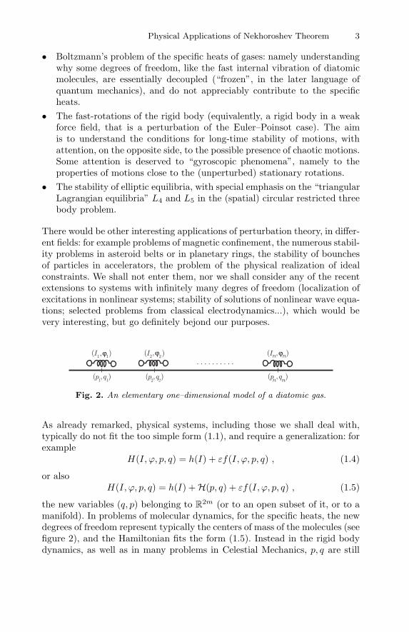
Fig. 2. An elementary one–dimensional model of a diatomic gas.
As already remarked, physical systems, including those we shall deal with,typically do not fit the too simple form (1.1), and require a generalization: forexample
H(I, ϕ, p, q) = h(I) + εf(I, ϕ, p, q) , (1.4)
or alsoH(I, ϕ, p, q) = h(I) +H(p, q) + εf(I, ϕ, p, q) , (1.5)
the new variables (q, p) belonging to R2m (or to an open subset of it, or to a
manifold). In problems of molecular dynamics, for the specific heats, the newdegrees of freedom represent typically the centers of mass of the molecules (seefigure 2), and the Hamiltonian fits the form (1.5). Instead in the rigid bodydynamics, as well as in many problems in Celestial Mechanics, p, q are still
4 Giancarlo Benettin
action–angle variables, but the actions do not enter the unperturbed Hamil-tonian, and this makes a relevant difference. The unperturbed Hamiltonian,if it does not depend on all actions, is said to be properly degenerate, and theabsent actions are themselves called degenerate. For the Kepler problem, thedegenerate actions represent the eccentricity and the inclination of the orbit;for the Euler-Poinsot rigid body they determine the orientation in space of theangular momentum. The perturbed Hamiltonian, for such systems, fits (1.4).Understanding the behavior of degenerate variables is physically important,but in general is not easy, and requires assumptions on the perturbation.3 Suchan investigation is among the most interesting ones in perturbation theory.
As a final introductory remark, let us comment the distinction, proposedin the title of these lectures, between “exponential estimates” and “Nekhoro-shev theorem”.4 As we shall see, some perturbative problems concern systemswith essentially constant frequencies. These include isochronous systems, butalso some anisochronous systems for which the frequencies stay neverthelessalmost constants during the motion, as is the case of molecular collisions.Such systems require only an analytic study: in the very essence, it is enoughto construct a single normal form, with an exponentially small remainder, toprove the desired result. We shall address these problems with the genericexpression “exponential estimates”. We shall instead deserve the more spe-cific expression “Nekhoroshev theorem”, or theory, for problems which areeffectively anisochronous, and require in an essential way, to be overcome,suitable geometric assumptions, like convexity or “steepness” of the unper-turbed Hamiltonian h (and occasionally assumptions on the perturbation,too). The geometrical aspects are in a sense the heart of Nekhoroshev theo-rem, and certainly constitute its major novelty. As we shall see, geometry willplay an absolutely essential role both in the study of the rigid body and inthe case of the Lagrangian equilibria.
These lectures are organized as follows: Section 2 is devoted to exponentialestimates, and includes, after a general introduction to standard perturbativemethods, some applications to molecular dynamics. It also includes an ac-count of an approximation proposed by Jeans and by Landau and Teller,which looks alternative to standard methods, and seems to work excellentlyin connection with molecular collisions. Section 3 is fully devoted to the Jeans–Landau–Teller approximation, which is revisited within a mathematically wellposed perturbative scheme. Section 4 contains an application of exponentialestimates to Statistical Mechanics, namely to the Boltzmann question aboutthe possible existence of long equilibrium times in classical gases. Section 5contains a general introduction to Nekhoroshev theorem. Section 6 is devoted3 This is clear if one considers, in (1.4), a perturbation depending only on (p, q):
these variables, for suitable f , can do anything on a time scale 1/ε.4 Such a distinction is not common in the literature, where the expression “Nekhoro-
shev theorem” is often ued as a synonymous of stability results for exponentiallylong times.
Physical Applications of Nekhoroshev Theorem 5
to the applications of Nekhoroshev theory to Euler–Poinsot perturbed rigidbody, while Section 7 is devoted to the application of the theory to ellipticequilibria, in particular to the stability of the so–called Lagrangian equilibriumpoints L4, L5 in the (spatial) circular restricted three body problem.
The style of the lectures will be occasionally informal; the aim is to providea general overview, with emphasis when possible on the connections betweendifferent applications, but with no possibility of entering details. Proofs willbe absent, or occasionally reduced to a sketch when useful to explain themost relevant ideas. (As is well known to researchers active in perturbationtheory, complete proofs are long, and necessarily include annoying parts, so forthem we forcely demand to the literature.) Besides rigorous results, we shallalso produce heuristic results, as well as numerical results; understanding aphysical system requires in fact, very often, the cooperation of all of theseinvestigation tools.
Most results reported in these lectures, and all the ideas underlying them,are fruit on one hand of many years of intense collaboration with Luigi Gal-gani, Antonio Giorgilli and Giovanni Gallavotti, from whom I learned, in theessence, all I know; on the other hand, they are fruit of the intense collab-oration, in the last ten years, with my colleagues Francesco Fasso and morerecently Massimiliano Guzzo. I wish to express to all of them my gratitude. Ialso wish to thank the director of CIME, Arrigo Cellina, and the director ofthe school, Antonio Giorgilli, for their proposal to give these lectures. I finallythank Massimiliano Guzzo for having reviewed the manuscript.
2 Exponential Estimates
We start here with a general result concerning exponential estimates in exactlyisochronous systems. Then we pass to applications to molecular dynamics, forsystems with either one or two independent frequencies.
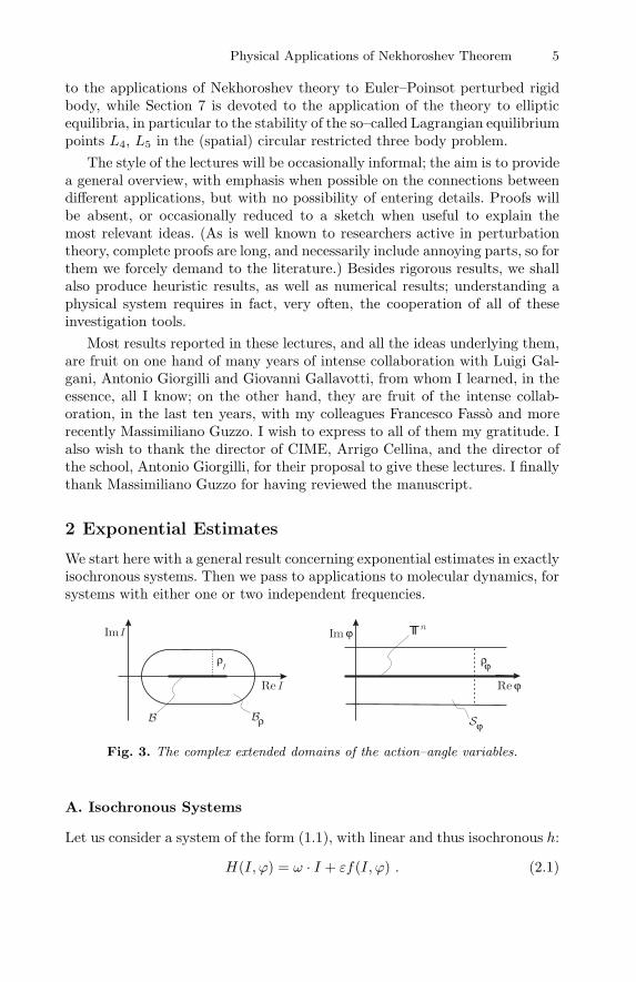
Fig. 3. The complex extended domains of the action–angle variables.
A. Isochronous Systems
Let us consider a system of the form (1.1), with linear and thus isochronous h:
H(I, ϕ) = ω · I + εf(I, ϕ) . (2.1)
6 Giancarlo Benettin
Given an “extension vector” = (I , ϕ), with positive entries, we define theextended domains (see figure 3)
∆(I) =
I ′ ∈ Cn : |I ′j − Ij | < I , j = 1, . . . , n
B =⋃
I∈B∆(I)
S =
ϕ ∈ Cn : | Imϕj | < ϕ, j = 1, . . . , n
D = B × S .(2.2)
Given two extension vectors and ′, inequalities of the form ′ ≤ areintended to hold separately on both entries. All functions we shall deal with,will be real analytic (that is analytic and real for real variables) in D′ , forsome ′ ≤ . Concerning norms, we make here the most elementary andcommon choices,5 and denote∥∥u∥∥∞′ = sup
(I,ϕ)∈D′|u(I, ϕ)| ,
∥∥v∥∥∞ = max
1≤j≤n|vj | , |ν| =
∑
j|νj | ,
respectively for u : D′ → C, for v ∈ Cn and for ν ∈ Z
n. By 〈 . 〉ϕ we shalldenote averaging on the angles.
A simple statement introducing exponential estimates for the isochronoussystem (2.1) is the following:
Proposition 1. Consider Hamiltonian (2.1), and assume that:
(a) f is analytic and bounded in D;(b) ω satisfies the “Diophantine condition”
|ν · ω| > γ
|ν|n ∀ν ∈ Zn , ν = 0 , (2.3)
for some positive constant γ;(c) ε is small, precisely
ε < ε∗ =C∥∥f∥∥∞
γInϕ,
for suitable C > 0.
Then there exists a real analytic canonical transformation (I, ϕ) = C(I ′, ϕ′),C : D 1
2→ D, which is small with ε:
∥∥I ′ − I
∥∥∞< c1 ε I ,
∥∥ϕ′ − ϕ
∥∥∞< c2 ε ϕ
(with suitable c1, c2 > 0), and gives the new Hamiltonian H ′ := H C thenormal form5 Obtaining good results requires in general the use of more sophisticated norms.
But final results can always be expressed (with worse constants) in terms of thesenorms.
Physical Applications of Nekhoroshev Theorem 7
H ′(I ′, ϕ′) = ω · I ′ + εg(I ′, ε) + ε e−(ε∗/ε)a R(I ′, ϕ′, ε) , (2.4)
with a = 1/(n+ 1) and
g = 〈f〉ϕ +O(ε) ,∥∥g∥∥∞12 ≤ 2
∥∥f∥∥∞,
∥∥R∥∥∞12≤∥∥f∥∥∞.
Such a statement (with some differences in the constants) can be foundfor example in [Ga1,BGa,GG,F1]; see also [B]. The optimal value 1/(n + 1)of the exponent a, which is the most crucial constant, comes from [F1]. Theinterest of the proposition is that the new actions I ′ are “exponentially slow”,
∥∥I∥∥∞ ∼ εe−(ε∗/ε)a
,
and consequently up to the large time |t| ∼ e(ε∗/ε)a
, also recalling∥∥I ′−I
∥∥∞ ∼
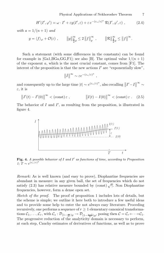
ε, it is∥∥I ′(t)− I ′(0)
∥∥∞< (const) ε ,
∥∥I(t)− I(0)
∥∥∞< (const) ε . (2.5)
The behavior of I and I ′, as resulting from the proposition, is illustrated infigure 4.
Fig. 4. A possible behavior of I and I ′ as functions of time, according to Proposition1; T ∼ e(ε∗/ε)a
Remark: As is well known (and easy to prove), Diophantine frequencies areabundant in measure: in any given ball, the set of frequencies which do notsatisfy (2.3) has relative measure bounded by (const)
√γ. Non Diophantine
frequencies, however, form a dense open set.Sketch of the proof. The proof of proposition 1 includes lots of details, butthe scheme is simple; we outline it here both to introduce a few useful ideasand to provide some help to enter the not always easy literature. Procedingrecursively, one performs a sequence of r ≥ 1 elementary canonical transforma-tions C1, . . . , Cr, with Cs : D(1− s
2r ) → D(1− s−12r ), posing then C = Cr · · ·C1.
The progressive reduction of the analyticity domain is necessary to perform,at each step, Cauchy estimates of derivatives of functions, as well as to prove
8 Giancarlo Benettin
convergence of series. After s steps one deals with a Hamiltonian Hs in normalform up to the order s ≤ r − 1, namely
Hs(I, ϕ) = h(I) + εgs(I, ε) + εs+1fs(I, ϕ, ε) , (2.6)
and operates in such a way to push the remainder fs one order further, thatis to get Hs+1 = Hs Cs+1 of the same form (2.6), but with s+ 1 in place ofs. To this end, the perturbation fs is split into its average 〈fs〉, which doesnot depend on the angles and can be progressively accumulated into g, andits zero-average part fs − 〈fs〉; the latter is then “killed” (at the lowest orders + 1) by a suitable choice of Cs+1. No matter how one decides to performcanonical transformations — the so-called Lie method is here recommended,but the traditional method of generating functions with inversion also works— one is confronted with the Hamilton–Jacobi equation, in the form
ω · ∂χ∂ϕ
= fs − 〈fs〉 , (2.7)
the unknown χ representing either the generating function or the the generatorof the Lie series (the auxiliary Hamiltonian entering the Lie method). Let usrecall that in the Lie method canonical transformations are defined as thetime–one map of a convenient auxiliary Hamiltonian flow, the new variablesbeing the initial data. In the problem at hand, to pass from order s to orders+1, we use an auxiliary Hamiltonian εsχ, and so, denoting its flow by Φtεsχ,the new Hamiltonian Hs+1 = Hs Φ1
εsχ is
Hs+1 = h+ εgs + εs+1fs + εs+1χ, h+O(εs+2) ;
developing the Poisson bracket, and recalling that ∂χ∂ϕ has zero average, (2.7)
follows.Equation (2.7) is solved by Fourier series,
χ(I, ϕ) =∑
ν∈Zn\0
fs,ν(I) eiν·ϕ
iν · ω ,
where fs,ν(I) are the Fourier coefficients of fs; assumption (b) is used todominate the “small divisors” ν ·ω, and it turns out that the series convergesand is conveniently estimated in the reduced strip S(1− s
2r ).This procedure works if ε is sufficiently small, and it turns out that at each
step the remainder reduces by a factor ελ, with
λ =c∥∥f∥∥∞rn+1
γInϕ,
c being some constant. (One must be rather clever to get here the optimalpower rn+1, and not a worse higher power. Complicated tricks must be intro-duced, see [F1].) The size of the last remainder fr is then, roughly,
Physical Applications of Nekhoroshev Theorem 9
εr+1λr ∼ ε (εrn+1)r∥∥f∥∥∞.
Quite clearly, raising r at fixed ε would produce a tremendous divergence.6
But clearly, it is enough to choose r dependent on ε, in such a way that (forexample) ελ e−1,
r ∼ ε−1/(n+1) ,
to produce an exponentially small remainder as in the statement of Propo-sition 1. It can be seen [GG] that this is nearly the optimal choice of r as afunction of ε, so as to minimize, for each ε, the final remainder. The situationresembles nonconvergent expansions of functions in asymptotic series. The“elementary” idea of taking r to be a function of ε, growing to infinity whenε goes to zero, is the heart of exponential estimates and of the analytic partof Nekhoroshev theorem.Remark: As we have seen, one proceeds as if the gain per step were a reductionof the perturbation by a factor ε (see (2.6)). This is indeed the prescription,but the actual gain at each step is practically much less, just a factor e−1.The point is that, due to the presence of small divisors, and to the necessityof making at each step Cauchy estimates with reduction of the analyticitydomain, the norm of fr grows very rapidly with r. The essence of the proofis to show that ‖fr‖ grows “only” as rr/a, with some positive a (as large aspossible, to improve the result). Such an apparently terrible growth gives riseto the desired exponential estimates, the final remainder decreasing as e−1/εa
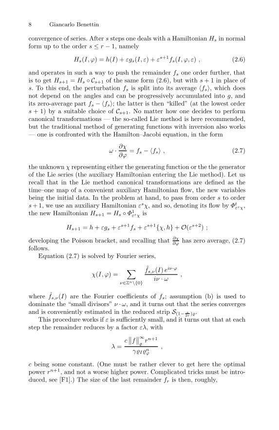
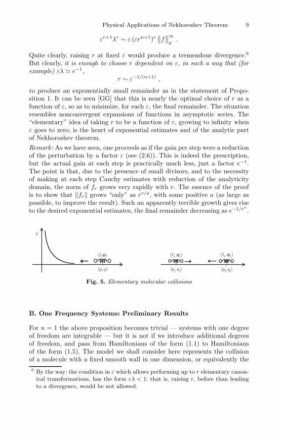
.
Fig. 5. Elementary molecular collisions
B. One Frequency Systems: Preliminary Results
For n = 1 the above proposition becomes trivial — systems with one degreeof freedom are integrable — but it is not if we introduce additional degreesof freedom, and pass from Hamiltonians of the form (1.1) to Hamiltoniansof the form (1.5). The model we shall consider here represents the collisionof a molecule with a fixed smooth wall in one dimension, or equivalently the6 By the way: the condition in ε which allows performing up to r elementary canon-
ical transformations, has the form ελ < 1: that is, raising r, before than leadingto a divergence, would be not allowed.
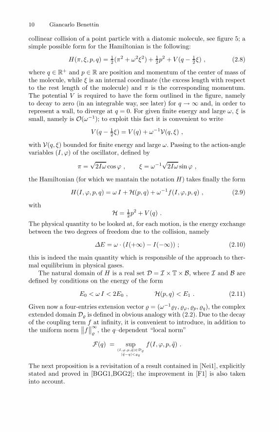
10 Giancarlo Benettin
collinear collision of a point particle with a diatomic molecule, see figure 5; asimple possible form for the Hamiltonian is the following:
H(π, ξ, p, q) = 12 (π2 + ω2ξ2) + 1
2p2 + V (q − 1
2ξ) , (2.8)
where q ∈ R+ and p ∈ R are position and momentum of the center of mass of
the molecule, while ξ is an internal coordinate (the excess length with respectto the rest length of the molecule) and π is the corresponding momentum.The potential V is required to have the form outlined in the figure, namelyto decay to zero (in an integrable way, see later) for q → ∞ and, in order torepresent a wall, to diverge at q = 0. For given finite energy and large ω, ξ issmall, namely is O(ω−1); to exploit this fact it is convenient to write
V (q − 12ξ) = V (q) + ω−1V(q, ξ) ,
with V(q, ξ) bounded for finite energy and large ω. Passing to the action-anglevariables (I, ϕ) of the oscillator, defined by
π =√
2Iω cosϕ , ξ = ω−1√
2Iω sinϕ ,
the Hamiltonian (for which we mantain the notation H) takes finally the form
H(I, ϕ, p, q) = ω I +H(p, q) + ω−1f(I, ϕ, p, q) , (2.9)
withH = 1
2p2 + V (q) .
The physical quantity to be looked at, for each motion, is the energy exchangebetween the two degrees of freedom due to the collision, namely
∆E = ω · (I(+∞)− I(−∞)) ; (2.10)
this is indeed the main quantity which is responsible of the approach to ther-mal equilibrium in physical gases.
The natural domain of H is a real set D = I × T× B, where I and B aredefined by conditions on the energy of the form
E0 < ω I < 2E0 , H(p, q) < E1 . (2.11)
Given now a four-entries extension vector = (ω−1I , ϕ, p, q), the complexextended domain D is defined in obvious analogy with (2.2). Due to the decayof the coupling term f at infinity, it is convenient to introduce, in addition tothe uniform norm
∥∥f∥∥∞
, the q–dependent “local norm”
F(q) = sup(I,ϕ,p,q)∈D
|q−q|<q
f(I, ϕ, p, q) .
The next proposition is a revisitation of a result contained in [Nei1], explicitlystated and proved in [BGG1,BGG2]; the improvement in [F1] is also takeninto account.
Physical Applications of Nekhoroshev Theorem 11
Proposition 2. Assume that:
i. H is analytic and bounded in D;ii. F(q), as defined above, dacays to zero in an integrable way for |q| → ∞;iii. ω is large, say ω > ω∗ with suitable ω∗.
Then there exists a canonical transformation (I, ϕ, p, q) = C(I ′, ϕ′, p′, q′), C :D 1
2→ D, small with ω−1 and reducing to the identity at infinity:
|I ′ − I| < ω−2F(q)I , |α′ − α| < ω−1F(q)α for α = ϕ, p, q ,
which gives the new Hamiltonian H ′ = H C the normal form
H ′(I ′, ϕ′, p′, q′) = ω I ′ +H(p′, q′) + ω−1g(I ′, p′, q′, ω)+ ω−1e−ω/ω∗ R(I ′, ϕ′, p′, q′) ,
(2.12)
with g = 〈f〉ϕ, and g, R bounded by
|g(I ′, ϕ′, p′, q′)| , |R(I ′, ϕ′, p′, q′)| < (const)F(q) .
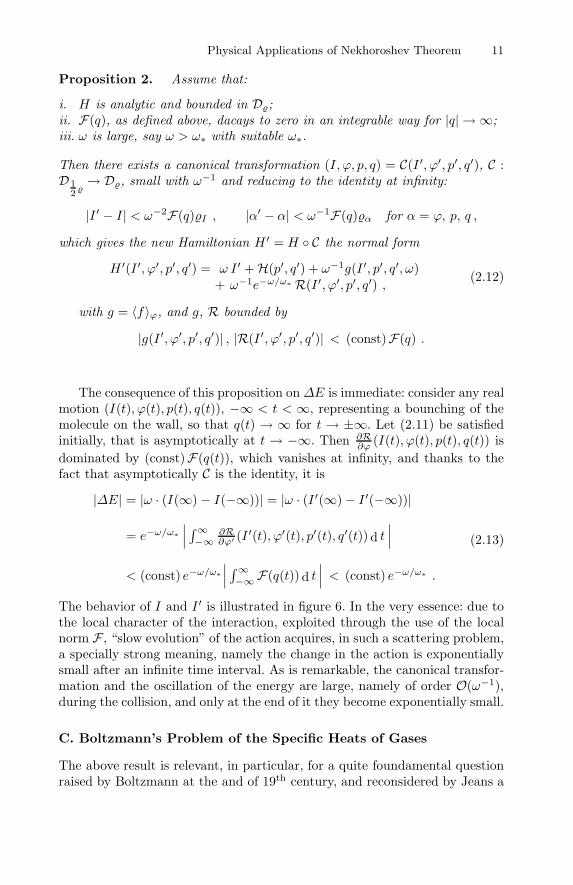
The consequence of this proposition on ∆E is immediate: consider any realmotion (I(t), ϕ(t), p(t), q(t)), −∞ < t < ∞, representing a bounching of themolecule on the wall, so that q(t) → ∞ for t → ±∞. Let (2.11) be satisfiedinitially, that is asymptotically at t → −∞. Then ∂R
∂ϕ (I(t), ϕ(t), p(t), q(t)) isdominated by (const)F(q(t)), which vanishes at infinity, and thanks to thefact that asymptotically C is the identity, it is
|∆E| = |ω · (I(∞) − I(−∞))| = |ω · (I ′(∞)− I ′(−∞))|
= e−ω/ω∗∣∣∣
∫∞−∞
∂R∂ϕ′ (I ′(t), ϕ′(t), p′(t), q′(t)) d t
∣∣∣
< (const) e−ω/ω∗∣∣∣
∫∞−∞F(q(t)) d t
∣∣∣ < (const) e−ω/ω∗ .
(2.13)
The behavior of I and I ′ is illustrated in figure 6. In the very essence: due tothe local character of the interaction, exploited through the use of the localnorm F , “slow evolution” of the action acquires, in such a scattering problem,a specially strong meaning, namely the change in the action is exponentiallysmall after an infinite time interval. As is remarkable, the canonical transfor-mation and the oscillation of the energy are large, namely of order O(ω−1),during the collision, and only at the end of it they become exponentially small.
C. Boltzmann’s Problem of the Specific Heats of Gases
The above result is relevant, in particular, for a quite foundamental questionraised by Boltzmann at the and of 19th century, and reconsidered by Jeans a
12 Giancarlo Benettin
Fig. 6. I and I ′ as functions of t, in molecular collisions
few years later, concerning the classical values of the specific heats of gases.One should recall that at Boltzmann’s time the molecular theory of gases wasfar from being universally accepted. In some relevant questions the theory wasindubitably succesful: in particular, via the equipartition principle, it providedthe well known mechanical interpretation of the temperature as kinetic energyper degree of freedom, and led to the celebrated link CV = f
2 R (R denotingthe usual constant of gases) between the constant-volume specific heat, whichcharachterizes the thermodynamics of an ideal gas, and the number f of de-grees of freedom of each molecule, thought of as a small mechanical device;more precisely, f is the number of quadratic terms entering the expression ofthe energy of a molecule.
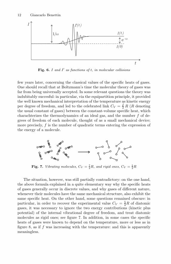
Fig. 7. Vibrating molecules, CV = 72R, and rigid ones, CV = 5
2R
The situation, however, was still partially contradictory: on the one hand,the above formula explained in a quite elementary way why the specific heatsof gases generally occur in discrete values, and why gases of different nature,whenever their molecules have the same mechanical structure, also exhibit thesame specific heat. On the other hand, some questions remained obscure: inparticular, in order to recover the experimental value CV = 5
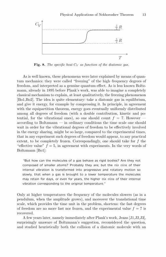
2R of diatomicgases, it was necessary to ignore the two energy contributions (kinetic pluspotential) of the internal vibrational degree of freedom, and treat diatomicmolecules as rigid ones; see figure 7. In addition, in some cases the specificheats of gases were known to depend on the temperature, more or less as infigure 8, as if f was increasing with the temperature: and this is apparentlymeaningless.
Physical Applications of Nekhoroshev Theorem 13
Fig. 8. The specific heat CV as function of the diatomic gas.
As is well known, these phenomena were later explained by means of quan-tum mechanics: they were called “freezing” of the high–frequency degrees offreedom, and interpreted as a genuine quantum effect. As is less known Boltz-mann, already in 1895 before Plank’s work, was able to imagine a completelyclassical mechanism to explain, at least qualitatively, the freezing phenomenon[Bo1,Bo2]. The idea is quite elementary: take a diatomic gas in equilibrium,and give it energy, for example by compressing it. In principle, in agreementwith the equipartition theorem, energy goes eventually uniformly distributedamong all degrees of freedom (with a double contribution, kinetic and po-tential, for the vibrational ones), so one should count f = 7. However —according to Boltzmann — in ordinary conditions the time scale one shouldwait in order for the vibrational degrees of freedom to be effectively involvedin the energy sharing, might be so large, compared to the experimental times,that in any experiment such degrees of freedom would appear, to any practicalextent, to be completely frozen. Correspondingly, one should take for f the“effective value” f = 5, in agreement with experiments. In the very words ofBoltzmann [Bo1]:
“But how can the molecules of a gas behave as rigid bodies? Are they not
composed of smaller atoms? Probably they are; but the vis viva of their
internal vibration is transformed into progressive and rotatory motion so
slowly, that when a gas is brought to a lower temperature the molecules
may retain for days, or even for years, the higher vis viva of their internal
vibration corresponding to the original temperature.”
Only at higher temperatures the frequency of the molecules slowers (as in apendulum, when the amplitude grows), and moreover the translational timescale, which provides the time unit in the problem, shortens: the fast degreesof freedom are no more fast nor frozen, and the experimental value f = 7 isrecovered.
A few years later, namely immediately after Plank’s work, Jeans [J1,J2,J3],surprisingly unaware of Boltzmann’s suggestion, reconsidered the question,and studied heuristically both the collision of a diatomic molecule with an
14 Giancarlo Benettin
unstructured atom, to understand the anomalous specific heats, and the re-lated problem of the lack of the “ultraviolet catastrophe” in the blackbodyradiation.7 Jeans’ purpose is to show that, in both cases, Plank’s quantizationwas unnecessary.8 Let us restrict ourselves to the former problem, forgettingthe too complicated question of the blackbody radiation. The heuristic con-clusion, or perhaps the convinciment reached by Jeans, is the following: if ϕo
denotes the asymptotic phase of the oscillator,
ϕo = limt→−∞
ϕ(t)− ωt , (2.14)
then the average 〈∆E〉ϕo of ∆E on ϕo follows an exponential law of the form
〈∆E〉ϕo ∼ e−τω , (2.15)
where τ is a convenient constant, not well defined but of the order of thecollision time. According to (2.15), for large ω — large “elasticity”, in Jeans’own words — equilibrium times could get enormously long:
“In other words, the ‘elasticity’ could easily make the difference between
dissipation of energy in a fraction of a second and dissipation in billions of
years.”
(dissipation means here transfer of energy to the internal degrees of freedom).
D. The Jeans-Landau-Teller (JLT) Approximationfor a Single Frequency
Further contributions to the problem of the energy exchanges with fast degreesof freedom in classical systems, came from Rutgers [Ru] and Landau and Teller[LT], around 1936.9 Quite surprisingly, these authors are unaware of both7 As is known, in conflict with experience and with the common sense, CV for the
blackbody was theoretically predicted to be infinite, with a diverging contribu-tion of the high frequencies, simply because of the infinite number of degrees offreedom.
8 Later on, however, Jeans reconsidered his point of view. Chapter XVI of his bookon gas theory [J3], where he better explains his point of view, is still present inthe 1916 second edition, but not in the 1920 third edition.
9 The very fundamental problem of quantization is obviously no more in discussionin 1936, but other problems, like the possible dependence of the velocity of soundon the frequency, were leading to the same question. In the very essence: thevelocity of sound depends on CV , and so if the effective CV depends on the timescale of the experiment, then the velocity of the low and of the high frequencysound waves (time scales of 10−1 and 10−4 sec respectively) could be different,with a possibly observable dispersion. By the way: most of the considerationcontained in [LT], concerning the dispersion of sound, are nearly identical tothose reported by Jeans in the first two editions of his book [J3].
Physical Applications of Nekhoroshev Theorem 15
Boltzmann and Jeans ideas. It is worthwhile to reconsider here [LT], althoughin a somehow revisited form (see also [Ra]). The approximation scheme of[LT] follows rather closely the ideas by Jeans, so we shall refer to it as to theJeans-Landau-Teller (JLT) approximation.
Consider again the Hamiltonian
H(I, ϕ, p, q) = ω I +H(p, q) + εf(I, ϕ, p, q) , (2.16)
which coincides with (2.9), but for the fact that ω−1 in front of the pertur-bation f is here replaced by the small parameter ε. As we shall see, it is veryuseful to treat ω and ε as independent parameters, recalling only at the endε = ω−1. Consider a motion (I(t), ϕ(t), p(t), q(t)), with asymptotic data fort→ −∞
I(t)→ Io , ϕ(t)− ωt→ ϕo , p(t)→ −po , q(t) + pot→ qo = 0 . (2.17)
Taking qo = 0 is not restrictive: it corresponds to fix the time origin, and givesmeaning to ϕo. One has obviously
∆E = ω∆I = ω ε
∫ ∞
−∞
∂f
∂ϕ(I(t), ϕ(t), p(t), q(t)) d t . (2.18)
The idea is that for small ε the motion is somehow close to the unperturbedmotion
I0(t) = Io , ϕ0(t) = ϕo + ωt , p0(t) , q0(t) , (2.19)
where (p0(t), q0(t)) is a solution of the (integrable) Hamiltonian problem H,with asymptotic data as in (2.17). Replacing (2.19) into (2.18) gives a kind of“first order” approximation
∆E ω∆I = ω ε
∫ ∞
−∞
∂f
∂ϕ(Io, ϕo + ωt, p0(t), q0(t)) d t .
In some special cases the integral can be explicitly computed. But quite gen-erally, see [BCS] for details, if p0(t), q0(t) are analytic, as functions of thecomplex time t, in a strip | Im t| < τ (this of course requires H to be ana-lytic), then it is
∆E = E0 +∑
ν>0
Eν cos(νϕo + αν) , (2.20)
with exponentially small Eν , namely
Eν = εEν e−ντω for ν = 0 , E0 = 0 . (2.21)
The coefficients Eν in principle depend on ω, but in a way much weakerthan exponential, and are practically treated as constants (the precise depen-dence of Eν on ω is related to the nature of the singularities of p0(t), q0(t)).
16 Giancarlo Benettin
Since E0 is the average, that is the most important quantity in the physicalproblem, the second of (2.21) is not satisfactory, and some inspection to higherorder contributions is mandatory; the result turns out to be,10 see Section 2,
E0 = O(
ε2 e−2τω)
. (2.22)
The JLT approximation is in agreement with the Proposition 2 above,but the result sounds much better: it has the form of an equality, though ap-proximate, rather than a less useful inequality; the exponential law appearsalready at first order, rather than at the end of a complicated procedure; thecrucial coefficient τ in the exponent has a clear definition, and is connected ina simple way to the unperturbed problem, while the constant ω∗ entering theproposition is more obscure (ω∗, precisely as ε∗ in Proposition 1, expressesthe divergence rate of the best perturbative series one is able to produce). Asis also remarkable and new, the JLT approximation provides different expo-nential laws for the different Fourier components of ∆E. The most importantcomponents are E0, namely the average, and E1, which provides the domi-nant contribution to the fluctuations. For large ω, however, fluctuations arerelatively large, that is E1 E0; this will be important, see section 4 below.Finally, it is worthwhile to mention that the JLT approximation naturallyextends to other systems, for example a system with a rotator in place of theoscillator [BCS],
H(I, ϕ, p, q) = 12I
2 +H(p, q) + εf(I, ϕ, p, q) ; (2.23)
the results for ∆E are practically identical to (2.20,2.21,2.22).
In front of such an appealing result, a natural question arises: is the heuris-tic procedure meaningful, and in some sense reliable? Before discussing theo-retically the approximation, and try to make it rigorous in suitable assump-tions, let us compare the results with accurate numerical computations. As amatter of fact, see [BGi,BF1,BChF1], the use of symplectic integration algo-rithms in scattering problems allows to compute reliably very small energyexchanges, as is necessary to test the exponential laws (2.21) and (2.22) on asufficiently wide range.11
10 On this point, both [LT] and its revisitation [Ra] are somehow weak: due to thefact that Cartesian coordinates are used instead of the action–angle ones, somesecond order terms spuriously enter the first order calculation, and are taken asthe result. This is surprising, since these terms are positive definite, as if theoscillator could continuously gain energy. A better procedure [BCG] shows thatall second order terms are indeed O(ε2e−2τω), but their coefficients can have anysign.
11 We cannot enter here the delicate problem of the accuracy of symplectic inte-grators, and demand for this point to the literature, in particular to [BGi,BF1].But it is worthwhile to recall here that the main tool to understand the behaviorof symplectic integration algorithms, in particular for scattering problems, comesprecisely from perturbation theory, and is a question of exponential estimates.
Physical Applications of Nekhoroshev Theorem 17
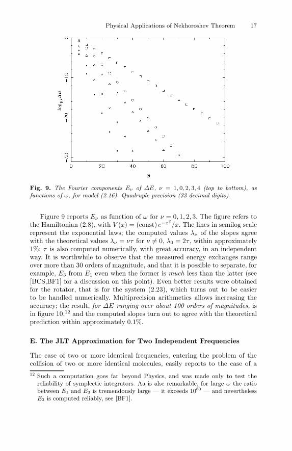
Fig. 9. The Fourier components Eν of ∆E, ν = 1, 0, 2, 3, 4 (top to bottom), asfunctions of ω, for model (2.16). Quadruple precision (33 decimal digits).
Figure 9 reports Eν as function of ω for ν = 0, 1, 2, 3. The figure refers tothe Hamiltonian (2.8), with V (x) = (const) e−x
2/x. The lines in semilog scale
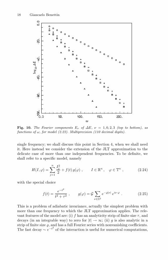
represent the exponential laws; the computed values λν of the slopes agreewith the theoretical values λν = ντ for ν = 0, λ0 = 2τ , within approximately1%; τ is also computed numerically, with great accuracy, in an independentway. It is worthwhile to observe that the measured energy exchanges rangeover more than 30 orders of magnitude, and that it is possible to separate, forexample, E3 from E1 even when the former is much less than the latter (see[BCS,BF1] for a discussion on this point). Even better results were obtainedfor the rotator, that is for the system (2.23), which turns out to be easierto be handled numerically. Multiprecision arithmetics allows increasing theaccuracy; the result, for ∆E ranging over about 100 orders of magnitudes, isin figure 10,12 and the computed slopes turn out to agree with the theoreticalprediction within approximately 0.1%.
E. The JLT Approximation for Two Independent Frequencies
The case of two or more identical frequencies, entering the problem of thecollision of two or more identical molecules, easily reports to the case of a12 Such a computation goes far beyond Physics, and was made only to test the
reliability of symplectic integrators. Aa is alse remarkable, for large ω the ratiobetween E1 and E3 is tremendously large — it exceeds 1060 — and neverthelessE3 is computed reliably, see [BF1].
18 Giancarlo Benettin
Fig. 10. The Fourier components Eν of ∆E, ν = 1, 0, 2, 3 (top to bottom), asfunctions of ω, for model (2.23). Multiprecision (110 decimal digits).
single frequency; we shall discuss this point in Section 4, when we shall needit. Here instead we consider the extension of the JLT approximation to thedelicate case of more than one independent frequencies. To be definite, weshall refer to a specific model, namely
H(I, ϕ) =n∑
j=1
I2j
2+ f(t) g(ϕ) , I ∈ R
n , ϕ ∈ Tn , (2.24)
with the special choice
f(t) =e−t
2
t2 + τ2, g(ϕ) = G
∑
ν∈Z2
e−|ν| eiν·ϕ . (2.25)
This is a problem of adiabatic invariance, actually the simplest problem withmore than one frequency to which the JLT approximation applies. The rele-vant features of the model are: (i) f has an analyticity strip of finite size τ , anddecays (in an integrable way) to zero for |t| → ∞; (ii) g is also analytic in astrip of finite size , and has a full Fourier series with nonvanishing coefficients.The fast decay ∼ e−t2 of the interaction is useful for numerical computations,
Physical Applications of Nekhoroshev Theorem 19
but has no other motivation; the very regular decay of the Fourier componentsof g simplifies the analysis. System (2.25) should be regarded as a simplifiedmodel for the collision of two rotating molecules.
The JLT approximation for this model is straightforward, namely, denotingas before by Io, ϕo the asymptotic data, it reads
∆Ij = −∫ ∞
−∞f(t)
∂g
∂ϕj(ϕo + Iot) d t .
The integration, for f, g as in (2.24), is also easy, and one finds
∆Ij =∑
ν∈Zn
Iν eiν·ϕ , (2.26)
withIν = c ν e−τ |ν·I
o|−|ν| , c = πτ−1eτ2. (2.27)
What is not easy instead is the analysis of such result, namely understandingwhich terms are small or large in (2.26). It must be stressed that in absenceof such analysis, the result is essentially formal and nearly empty. We are ableto proceed only in the simple case n = 2, Io = λΩ, for fixed Ω ∈ R
2 and largeλ ∈ R
+, so that the expression for I takes the form
Iν = c ν e−λτ |ν·Ω|−|ν| . (2.28)
Similar expressions can be found in [Ga2,S,DGJS] (in connection with thesplitting of separatrices, a problem which turns out to be strongly related), andin [BCG,BCaF]. Still, for a generic Ω ∈ R
2, the analysis is too difficult, andthe situation gets clear only under additional assumptions on Ω, of arithmeticcharacter. Following [BCaF], we consider here the special case Ω = (1,
√2),
and proceed heuristically (for a rigorous treatement of a similar situation,focused on the asymptotic behavior of the series for large λ, see [DGJS]).
A little reflection shows that, for large λ, the coefficients Iν entering thesum (2.26) have very different size. The largest ones are those for which ν ·Ωis small, that is the corresponding ν = (ν1, ν2) are such that −ν1/ν2 is a goodrational approximation of
√2. The theory of continued fraction provides then
the following sequence13 of ν’s:
(1,−1) , (3,−2) , (7,−5) , (17,−12) , (41,−29) , . . .
For each ν in such a “resonant sequence”, it is convenient to report log ‖Iν‖(euclidean norm) versus λ in logarithmic scale; this gives for each ν a straightline
log ‖Iν‖ = −ανλ− βν ,13 The rule, for Ω = (1,
√2), is that the sequence starts with (1,−1) and (ν1,−ν2)
is followed by (ν1 + 2ν2,−ν1 − ν2).
20 Giancarlo Benettin
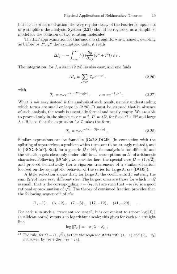
Fig. 11. The amplitudes ‖Iν‖ vs. λ, for ν in the resonant sequence, according tothe JLT approximation.
withαν = |ν ·Ω| , βν = |ν|+ log ‖ν‖+ log c .
Note that, proceding in the sequence, αν lowers, while βν increases, so the linesare as in figure 11 (the terms Iν , with ν out of the sequence, would producemuch lower lines, and correspondingly negligible contributions). Quite clearly,even inside the sequence, the different terms have very different size, andpractically, for each λ, just one of them dominates, with the only exceptionof narrow crossover regions around the intersection of the lines, where twonearby terms are comparable. The conclusion is that, if we forget crossoverand denote by ν(λ) the ν giving for each λ the dominant contribution, thenthe quantity of physical interest
∆maxI = maxϕo∈T2
‖∆I‖
follows the elementary law
∆maxI ‖Iν(λ)‖ . (2.29)
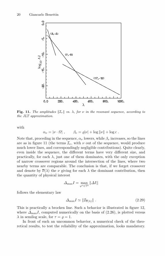
This is practically a brocken line. Such a behavior is illustrated in figure 12,where ∆maxI, computed numerically on the basis of (2.26), is plotted versusλ in semilog scale, for τ = = 1.
In front of such an uncommon behavior, a numerical check of the theo-retical results, to test the reliability of the approximation, looks mandatory.
Physical Applications of Nekhoroshev Theorem 21
Fig. 12. A numerical plot of ∆maxI. The curve resembles a brocken line, thoug itis not.
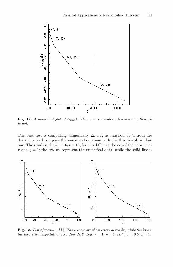
The best test is computing numerically ∆maxI, as function of λ, from thedynamics, and compare the numerical outcome with the theoretical brockenline. The result is shown in figure 13, for two different choices of the parameterτ and = 1; the crosses represent the numerical data, while the solid line is
Fig. 13. Plot of maxϕo ‖∆I‖. The crosses are the numerical results, while the line isthe theoretical expectation according JLT. Left: τ = 1, = 1; right: τ = 0.5, = 1.
22 Giancarlo Benettin
the theoretical expectation. The agreement looks pretty good. Let us stressthat all constants in (2.26) and (2.27) are determined, with no free parametersto be adjusted. For a more quantitative test, one can compare the measuredvalues of the constants αν and βν , obtained by a least square fit of the exper-imental data, with the theoretical expressions above; another quantity whichcan be tested is the ratio γν = ∆I2/∆I1, which, according to (2.28), should beν2/ν1 when Iν dominates. The results of the test are reported in the Table,for different values of the constants τ and , and for different dominant ν; α,β and γ are there the theoretical values, while α′, β′ and γ′ are the corre-sponding computed values. The agreement between theoretical and computedquantities looks excellent, in some cases (for γ) even impressive.
Also in this case of two frequencies, one can compare the outcome ofthe JLT approximation with rigorous inequalities obtained within traditionalperturbation theory. What it is easily proved rigorously is a proposition likethe following:
Proposition 3. Let H be as in (2.24), with f , g as in (2.25). Consider amotion with I(−∞) = λΩ, and Ω ∈ R
2 such that, for some γ > 0,
|ν ·Ω| > γ
|ν| . (2.30)
Then there exists λ∗ > 0 such that, if λ > λ∗, it is
‖I(+∞)− I(−∞)‖ < (const)λ−1e−( λλ∗ )1/2
. (2.31)
The Table
τ ν α α′ β β′ γ γ′
1.0 1.0 (7,-5) 0.0711 0.0709 7.70 7.76 1.400000 1.400003(17,-12) 0.02942 0.02943 23.82 23.83 1.416666 1.416666
0.5 1.0 (7,-5) 0.03554 0.03551 7.76 7.78 1.40000 1.40001(17,-12) 0.01472 0.01473 23.87 23.88 1.4166666 1.4166666
1.0 0.5 (17,-12) 0.02944 0.02945 9.320 9.325 1.416666 1.416666(41,-29) 0.0122 0.0124 28.9 28.4 1.4193793 1.4193793
1.0 0.25 (17,-12) 0.0294 0.0296 2.07 2.10 1.4166 1.4165(41,-29) 0.0122 0.0122 11.4 11.1 1.4137931 1.4137931
The strong Diophantine condition (2.30) is satisfied by a zero measure un-countable set14 in R
2, including Ω = (1,√
2). Such a restriction allows to get(λ/λ∗)a with a = 1
2 in (2.31).
14 To have a positive measure set in the space of frequencies, the denominator atthe r.h.s. of (2.30) needs to be |ν|n−1+ϑ, ϑ > 0, n being the number of frequencies(n = 2 in the problem at hand). The optimal exponent of λ in the exponentiallaw is then a = 1/(n+ ϑ).
Physical Applications of Nekhoroshev Theorem 23
The inequality (2.31) can be compared with the asymptotic behavior, forlarge λ, of (2.24). The latter is studied rigorously in [DGJS], and heuristicallyin [S,BCaF]; the result is
‖∆I‖ A eτ2
τ
√
λ
λ0(1 +O(
√λ)) e−
√λ/λ0 , λ−1
0 = (2 +√
2)τ ,
with A =√
3(√
2−1)π/2. Quite clearly, the JLT approximation is compatiblewith rigorous perturbation theory. But clearly, there is no comparison in theaccuracy and power of results.
The next Sections 3 and 4 are fully devoted to further considerations onthe JLT approximation.
3 A Rigorous Version of the JLT Approximationin a Model
A. Lindstedt Series Versus Von Zeipel Series
It is practically impossible, using the standard procedure of classical pertur-bation theory outlined in Section 2-A, to go beyond results in the form ofupper bounds like (2.5) or (2.13), for the obvious reason that the higher orderterms in g and in the remainder R, in the normal forms (2.4) or (2.12), arehardly known exactly, and only their norms are easily controlled. To produce“exact estimates”, that is narrow two-sided inequalities, it is mandatory toavoid chains of canonical transformations, and look directly at the behaviorof the solutions, specifically of I(t). This however is difficult: as is clear for ex-ample from figure 6 (for definiteness, we refer here to molecular collisions) I is“large”, namely is O(ε) or O(ω−1), and a final exponential estimate, with noaccumulation of deviations, requires taking into consideration compensationsamong deviations.
As a matter of fact, a branch of perturbation theory based on series ex-pansions of the solution in the original variables, without canonical transfor-mations, does exits, and is known in the literature as “Lindstet method”, ormethod of Lindstet series. It is among the oldest branches of perturbation the-ory, but it was soon abandoned in favor of the “von Zeipel method”, namelythe method based on canonical transformations and normal forms, becausethe series developments appared to conduce quite rapidly to huge amounts ofterms, rather difficult to handle, and to apparently unavoidable divergences.
Nowadays, after the work of Eliasson [E] who showed how to overcomethese difficulties, Lindsted series had a kind of revival, and are presently usedboth in KAM theory and in the related problem of the “splitting of separa-trices” in forced pendula or similar systems. A rigorous analysis of the JLTapproximation by means of Lindstet series was produced in [BCG]; as a matterof fact, the example there treated seems to be the simplest possible applicationof the Lindsted method. In this section we shall explain such result.
24 Giancarlo Benettin
The Hamiltonian studied in [BCG] is
H(I, ϕ, p, q) = ωI +H(p, q) + εg(ϕ)V (q) , H(p, q) =p2
2m+ U(q) ,
withI ∈ R , ϕ ∈ T
1 , (p, q) ∈ R2 .
Thanks to the fact that the perturbation is independent of I, so that themotion of ϕ is, trivially,
ϕ(t) = ϕo + ωt , (3.1)
such a model does not really represent the behavior of a diatomic moleculein an external potential, rather the behavior of a point mass, with a super-imposed periodic force F = −εg(ϕo +ωt)V ′(q). However, as shown in [BCG],the generalization to a generic perturbation V (I, ϕ, p, q) is possible, and eveneasy, as well as the generalization to the case (I, ϕ) ∈ R
n × Tn. But the lan-
guage and the notation get complicated, while no new ideas are added, sowe prefer to treat here only the simplest case. Concerning the choice of thepotentials U and V , we shall make here, as in [BCG], the easy choice
U(q) = V (q) = U0 e−q/d , (3.2)
which allows explicit computations. The constants U0, d and m will be takenrespectively as units of energy, length and mass, and so put equal to one fromnow on.
The quantity of interest, we recall, is
∆E = ωI(t)∣∣∣
∞
t=−∞= −H(p(t), q(t))
∣∣∣
∞
t=−∞
as function of the asymptotic data of the trajectory at t = −∞.
B. The Energy–Time Variables
First of all, it is convenient to introduce for the translational degree of free-dom new canonical variables in place of (p, q), precisely the energy–time vari-ables (η, ξ); these are the analog, for unbounded motions, of the more familiaraction–angle variables. To this purpose, consider any solution
p0(η, t) , q0(η, t)
of the Hamilton equations for H, such that asymptotically the translationalenergy is η, i.e. p(−∞) = −
√2η. Solutions with the same η are identical up
to the choice of the time origin; the one symmetric in time turns out to be
p0(η, t) =√
2η tanh√η
2t , q0(η, t) = log
(cosh√
η/2 t)2
η. (3.3)
Physical Applications of Nekhoroshev Theorem 25
We interpret these expressions as a change of variables, namely we pass from(p, q) to the new variables (η, ξ) by the (canonical) substitution
p = p0(η, ξ) , q = q0(η, ξ) .
It is obviously H(p0(η, ξ), q0(η, ξ)) = η, while correspondingly the new Hamil-tonian K(I, ϕ, η, ξ) = H(I, ϕ, p0(η, ξ), q0(η, ξ)) takes the form
K(I, ϕ, η, ξ) = ωI + η + εg(ϕ)f(η, ξ) ,
withf(η, ξ) =
η
(cosh√
η/2 ξ)2. (3.4)
An inspection to (3.3) shows that the domain of analyticity of the transfor-mation, and thus of f , is for any η > 0
| Im ξ| < τ(η) = π/√
2η (3.5)
(the singularities nearest to the real axis are second order poles in ξ = ±iτ).The energy exchange ∆E reads, in these new notations,
∆E = −∆η = −η(+∞) + η(−∞) .
Using (3.1), the Hamilton equations associated toK practically reduce to onlyone pair of time–dependent equations for η and ξ, namely
η = εg(ϕo + ωt)fη(η, ξ) , ξ = εg(ϕo + ωt)fξ(η, ξ) , (3.6)
withfη = −∂f
∂ξ, fξ =
∂f
∂η. (3.7)
Such form of fη, fξ reflects the Hamiltonian character of the problem. This,however, plays no role in the construction of Linstedt series, which are nat-urally more general, and is useful only occasionally, to show that a huge setof individually large terms, entering ∆η, exactly vanish. So, for the only saketo be clear, we shall proceed with generic fη, fξ, and recall (3.7) only whennecessary. The functions fη, fξ will be characterized by their analyticity prop-erties, and for the fact that they vanish, in an integrable way, for ξ → ∞, soas to represent a collision.
C. The Result
Consider a motion η(t), ξ(t) such that, asymptotically for t→ −∞,
η(t)→ ηo , ξ(t)− t→ 0 ,
and expand it in power series of ε around the unperturbed motion η0(t) = ηo,ξ0(t) = t:
26 Giancarlo Benettin
η(t) = ηo +∞∑
h=1
εhηh(t) , ξ(t) = t+∞∑
h=1
εhξh(t) . (3.8)
The series (in such a collisional problem) turn out to be convergent, for smallε, uniformly in t. Denote by ηh,ν , ξh,ν , ν ∈ Z, the Fourier components, withrespect to ϕ0, respectively of ηh(+∞) and ξh(+∞). In these notations it isthen
∆E = −∑
ν∈Z
Eν eiνϕo
, Eν =∞∑
h=1
εhηh,ν . (3.9)
By replacing (3.8) into the equations of motions (3.6), one finds a hierarchyof equations for ηh, ξh, complicated to write but conceptually easy. The firstorder is straightforward: one just uses inside fη and fξ, in the equations ofmotion (3.6), the unperturbed motion η(t) = ηo, ξ(t) = t, thus getting, forexample for η,
η1 = fη(ηo, t)g(ϕo + ωt) , η1(t) =∫ t
−∞fη(ηo, t′)g(ϕo + ωt′) dt′ . (3.10)
This is precisely the JLT approximation, rewritten in the (η, ξ) variables. Ac-tually if
g(ϕ) =∑
ν∈Z
gν eiνϕ ,
then one immediately deduces
η1(+∞) =∑
ν∈Z
η1,ν eiνϕo
, η1,ν = gν
∫ ∞
−∞fη(ηo, t)eiνωt dt .
For ν = 0, by simply recalling that fη is analytic, as function of ξ, as far as(3.5) is satisfied, one then gets
η1,ν ∼ gν e−τ |ν|ω .
Such an exponential law is useless for ν = 0: but thanks to the Hamiltoniancharacter of the problem, i.e. to the first of (3.7), it turns out that η1,0 exactlyvanishes:
η1,0 = −g0∫ ∞
−∞
∂f
∂tdt = −g0V (q(t))
∣∣∣
∞
t=−∞= 0 . (3.11)
For f as in (3.4), the integral for the dominant term η1,1 can be explicitlycomputed, namely
η1,1 = 4πig1ω2
eτω − e−τω ,
and so
∆E = 8πg1ε ω2
eτω − e−τω sinϕo + · · · .
Physical Applications of Nekhoroshev Theorem 27
Similar expressions are found for ξ1; the average ξ1,0, however, in general doesnot vanish.
Let us now proceed beyond the first order. The complete hierarchy ofequations reads, for α either η or ξ:
αh(t) =∫ t
−∞Fα,h(t′) dt′ , (3.12)
withFα,1(t) = g(ϕo + ωt)fα(ηo, t) , (3.13)
and for h > 1:
Fα,h(t)=g(ϕo + ωt)h−1∑
m=1
m∑
j=0
fm,jα (ηo, t)∑
k1,...,km≥1|k|=h−1
ξk1 (t)· · ·ξkj (t)ηkj+1 (t)· · ·ηkm(t),
(3.14)where |k| =
∑
i ki, while fm,jα is the coefficient entering the Taylor expansionof fα,
fm,jα =1
j!(m− j)!∂mfα
∂ξj∂ηm−j .
The procedure to be followed is now this:
(a) Proving convergence of all expansions, uniformly in t, for sufficientlysmall ε.
(b) Working out conditions such that the lowest order term η1,ν , for ν = 0,dominates the series (3.9) for Eν . This requires, in particular, that at anyorder h in ε the coefficients ηh,ν have at least a factor e−|ν|τω in front.
(c) Proving that for ν = 0 the Hamiltonian symmetry leads to a cancellation,which generalizes (3.11): among terms contributing to E0, only those within front a factor e−2τω (or smaller) survive, while individually larger termsexactly sum to zero.
The assumptions which are needed are the following: concerning g, it is sup-posed to be analytic and bounded in a strip | Imϕ| < , for some positive ;without loss of generality, we can assume that g is bounded by 1 in the strip,so that
|gν | ≤ e−|ν| . (3.15)
Concerning fη, fξ, the technical assumption that turns out to be useful, and issatisfied by f as in (3.4), is that the coefficients fm,jα are analytic, as functionsof ξ, in a strip | Im ξ| < τ(η), and in any smaller strip | Im ξ| < (1 − δ)τ(η),δ > 0, they are bounded by an expression of the form
|fm,jα (η, s+ iσ)| ≤ Cmδ−m−m0w(s) (3.16)
28 Giancarlo Benettin
with some C > 0, m0 > 0 and∫ ∞
−∞w(s) d s = A <∞ . (3.17)
A little reflections shows that these hypotheses are indeed natural in thisproblem, and just make quantitative two elementary facts: (i) For given η,the unperturbed motion q(t) is analytic for | Im t| < τ(η), with τ as in (3.5);Cauchy estimates then easily lead to (3.16). (ii) Along any unperturbed mo-tion, the coupling term V (q(t)) vanishes in an integrable way for t → ±∞.For the potentials (3.2), one computes m0 = 3.
Proposition 1. In the above assumptions, denoting
B = 8CA , m1 = m0 + 1 ,
the following holds:
i. For |ε| < B−1 the series (3.8) converge, namely it is
|ηh(t)| , |ξh(t)| ≤ ABh−1 .
ii. The Fourier components ηh,ν and ξh,ν , respectively of ηh(+∞) andξh(+∞), satisfy the δ–corrected exponential estimates
|ηh,ν | |ξh,ν | ≤ ABh−1δ−hm1+1 e−|ν|τ(1−δ)ω−|ν| , (3.18)
for any δ ∈ (0, 1).iii. In the Hamiltonian case, the average ηh,0 satisfies the special exponential
estimate|ηh,0| ≤ ABh−1δ−hm1+1 e−2τ(1−δ)ω . (3.19)
Comments:
1. The presence of the correction (1 − δ) at the exponents in the estimates(3.18) shows that points (b), (c) of the above program are fulfilled only ifε is specially small, namely
ε < (const)ω−m1 ; (3.20)
indeed, in order for the correction to disappear, in such a way that the firstorder (which is exactly computed and has no correction) dominates, onemust take δ ∼ ω−1, but then (3.20) is necessary to ensure convergence.
2. If instead, as in the physical problem of molecular collisions, one has onlyε = ω−1, then only upper estimates to the energy exchange can be workedout. Such upper estimates are quite interesting, and full in agreement withnumerical computations: in particular, taking δ = ε1/(2m1) = ω−1/(2m1),for ω > B2 one gets
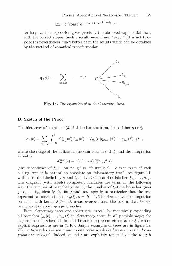
Physical Applications of Nekhoroshev Theorem 29
|Eν | < (const) e−|ν|ωτ(1−ω−1/(2n))−ν ;
for large ω, this expression gives precisely the observed exponential laws,with the correct slopes. Such a result, even if non “exact” (it is not two–sided) is nevertheless much better than the results which can be obtainedby the method of canonical transformation.
Fig. 14. The expansion of ηh in elementary trees.
D. Sketch of the Proof
The hierarchy of equations (3.12–3.14) has the form, for α either η or ξ,
αh(t) =∑
m,j,k
∫ t
−∞Kαm,j(t′) ξk1(t′) · · · ξkj (t
′)ηkj+1 (t′) · · · ηkm(t′) d t′ ,
where the range of the indices in the sum is as in (3.14), and the integrationkernel is
Km,jα (t) = g(ϕo + ωt)fm,jα (ηo, t)
(the dependence of Km,jα on ϕo, ηo is left implicit). To each term of sucha huge sum it is natural to associate an “elementary tree”, see figure 14,with a “root” labelled by α and t, and m ≥ 1 branches labelled ξk1 , . . . , ηkm .The diagram (with labels) completely identifies the term, in the followingway: the number of branches gives m; the number of ξ–type branches givesj; k1, . . . , km identify the integrand, and specify in particular that the treerepresents a contribution to αh(t), h = |k|−1. The circle stays for integrationon time, with kernel Km,jα . To avoid overcounting, the rule is that ξ–typebranches stay above η-type branches.
From elementary trees one constructs “trees”, by recursively expandingall branches ξk1(t) . . . , ηkm(t) in elementary trees, in all possible ways; theexpansion ends when all the end–branches represent either η1 or ξ1, whoseexplicit expressions are in (3.10). Simple examples of trees are in figure 15.Elementary rules provide a one to one correspondence between trees and con-tributions to αh(t). Indeed, α and t are explicitly reported on the root; h
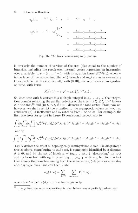
30 Giancarlo Benettin
Fig. 15. The trees contributing to η2 and η3.
is precisely the number of vertices of the tree (also equal to the number ofbranches, including the root); each internal vertex represents an integrationover a variable tv, v = 0, . . . , h− 1, with integration kernel Km,jα (tv), where αis the label of the outcoming (the left) branch and m, j are as in elementarytrees; each end vertex v, coherently with (3.10), also represents an integrationon time, with kernel
K0,0α (tv) = g(ϕo + ωtv)fα(ηo, tv) .
So, each tree with h vertices is a multiple integral in t0, . . . , th−1, the integra-tion domain reflecting the partial ordering of the tree: (i) t′v ≤ tv if v′ followsv in the tree,15 and (ii) t0 ≤ t, if v = 0 denotes the root vertex. From now on,however, we shall restrict the attention to the asymptotic values αh(+∞), socondition (ii) is ineffective and t0 extends from −∞ to ∞. For example, thefirst two trees for η3(∞) in figure 15 corrispond respectively to∫ ∞
−∞d t0
∫ t0
−∞d t1
∫ t0
−∞d t2f
2,1η (ηo, t0)fξ(η
o, t1)fη(ηo, t2)g(ϕo + ωt0)g(ϕ
o + ωt1)g(ϕo + ωt2)
and to∫ ∞
−∞d t0
∫ t0
−∞d t1
∫ t1
−∞d t2 f
2,1η (ηo, t0)fξ(η
o, t1)fξ(ηo, t2)g(ϕ
o + ωt0)g(ϕo + ωt1)g(ϕ
o + ωt2).
Let Θ denote the set of all topologically distinguishable tree–like diagrams; atree as above, contributing to αh(+∞), is completely identified by a diagramϑ ∈ Θ, and by the set of labels α = (α0, . . . , αh−1) “decorating” its rootand its branches, with α0 = α and α1, . . . , αh−1 arbitrary, but for the factthat among the branches issuing from the same vertex, ξ–type ones must stayabove η–type ones. One can then write
αh(+∞) =∑
ϑ∈Θ
∑
α:α0=α
V (ϑ, α) ,
where the “value” V (ϑ, α) of the tree is given by15 In any tree, the vertices constitute in the obvious way a partially ordered set.
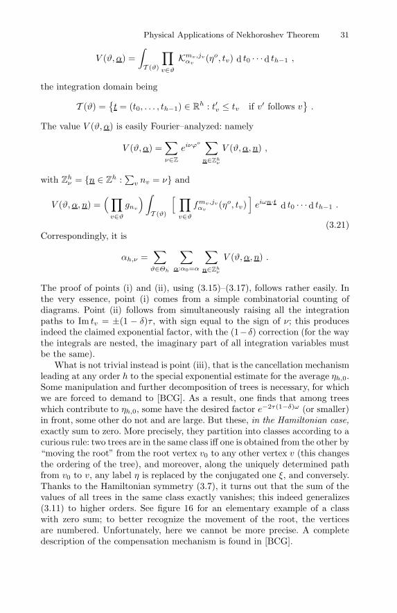
Physical Applications of Nekhoroshev Theorem 31
V (ϑ, α) =∫
T (ϑ)
∏
v∈ϑKmv ,jvαv
(ηo, tv) d t0 · · · d th−1 ,
the integration domain being
T (ϑ) =
t = (t0, . . . , th−1) ∈ Rh : t′v ≤ tv if v′ follows v
.
The value V (ϑ, α) is easily Fourier–analyzed: namely
V (ϑ, α) =∑
ν∈Z
eiνϕo ∑
n∈Zhν
V (ϑ, α, n) ,
with Zhν = n ∈ Z
h :∑
v nv = ν and
V (ϑ, α, n) =(∏
v∈ϑgnv
)∫
T (ϑ)
[ ∏
v∈ϑfmv,jvαv
(ηo, tv)]
eiωn·t d t0 · · · d th−1 .
(3.21)Correspondingly, it is
αh,ν =∑
ϑ∈Θh
∑
α:α0=α
∑
n∈Zhν
V (ϑ, α, n) .
The proof of points (i) and (ii), using (3.15)–(3.17), follows rather easily. Inthe very essence, point (i) comes from a simple combinatorial counting ofdiagrams. Point (ii) follows from simultaneously raising all the integrationpaths to Im tv = ±(1 − δ)τ , with sign equal to the sign of ν; this producesindeed the claimed exponential factor, with the (1−δ) correction (for the waythe integrals are nested, the imaginary part of all integration variables mustbe the same).
What is not trivial instead is point (iii), that is the cancellation mechanismleading at any order h to the special exponential estimate for the average ηh,0.Some manipulation and further decomposition of trees is necessary, for whichwe are forced to demand to [BCG]. As a result, one finds that among treeswhich contribute to ηh,0, some have the desired factor e−2τ(1−δ)ω (or smaller)in front, some other do not and are large. But these, in the Hamiltonian case,exactly sum to zero. More precisely, they partition into classes according to acurious rule: two trees are in the same class iff one is obtained from the other by“moving the root” from the root vertex v0 to any other vertex v (this changesthe ordering of the tree), and moreover, along the uniquely determined pathfrom v0 to v, any label η is replaced by the conjugated one ξ, and conversely.Thanks to the Hamiltonian symmetry (3.7), it turns out that the sum of thevalues of all trees in the same class exactly vanishes; this indeed generalizes(3.11) to higher orders. See figure 16 for an elementary example of a classwith zero sum; to better recognize the movement of the root, the verticesare numbered. Unfortunately, here we cannot be more precise. A completedescription of the compensation mechanism is found in [BCG].
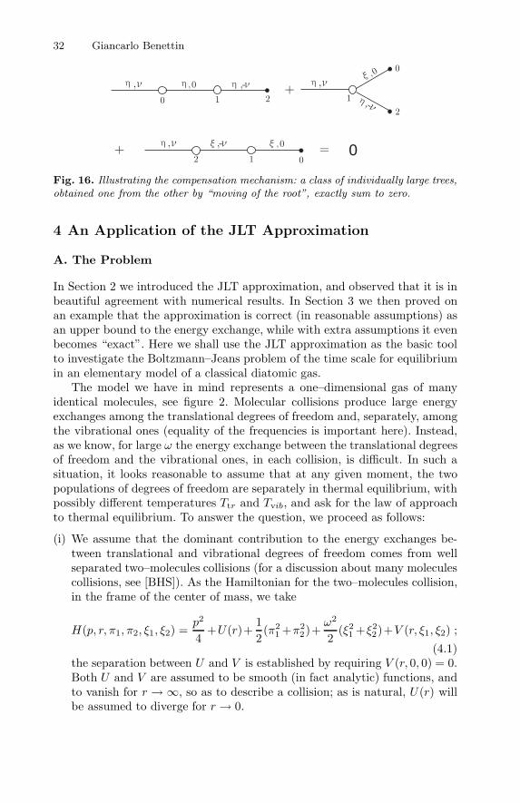
32 Giancarlo Benettin
Fig. 16. Illustrating the compensation mechanism: a class of individually large trees,obtained one from the other by “moving of the root”, exactly sum to zero.
4 An Application of the JLT Approximation
A. The Problem
In Section 2 we introduced the JLT approximation, and observed that it is inbeautiful agreement with numerical results. In Section 3 we then proved onan example that the approximation is correct (in reasonable assumptions) asan upper bound to the energy exchange, while with extra assumptions it evenbecomes “exact”. Here we shall use the JLT approximation as the basic toolto investigate the Boltzmann–Jeans problem of the time scale for equilibriumin an elementary model of a classical diatomic gas.
The model we have in mind represents a one–dimensional gas of manyidentical molecules, see figure 2. Molecular collisions produce large energyexchanges among the translational degrees of freedom and, separately, amongthe vibrational ones (equality of the frequencies is important here). Instead,as we know, for large ω the energy exchange between the translational degreesof freedom and the vibrational ones, in each collision, is difficult. In such asituation, it looks reasonable to assume that at any given moment, the twopopulations of degrees of freedom are separately in thermal equilibrium, withpossibly different temperatures Ttr and Tvib, and ask for the law of approachto thermal equilibrium. To answer the question, we proceed as follows:
(i) We assume that the dominant contribution to the energy exchanges be-tween translational and vibrational degrees of freedom comes from wellseparated two–molecules collisions (for a discussion about many moleculescollisions, see [BHS]). As the Hamiltonian for the two–molecules collision,in the frame of the center of mass, we take
H(p, r, π1, π2, ξ1, ξ2) =p2
4+U(r)+
12(π2
1 +π22)+
ω2
2(ξ21 +ξ22)+V (r, ξ1, ξ2) ;
(4.1)the separation between U and V is established by requiring V (r, 0, 0) = 0.Both U and V are assumed to be smooth (in fact analytic) functions, andto vanish for r → ∞, so as to describe a collision; as is natural, U(r) willbe assumed to diverge for r → 0.
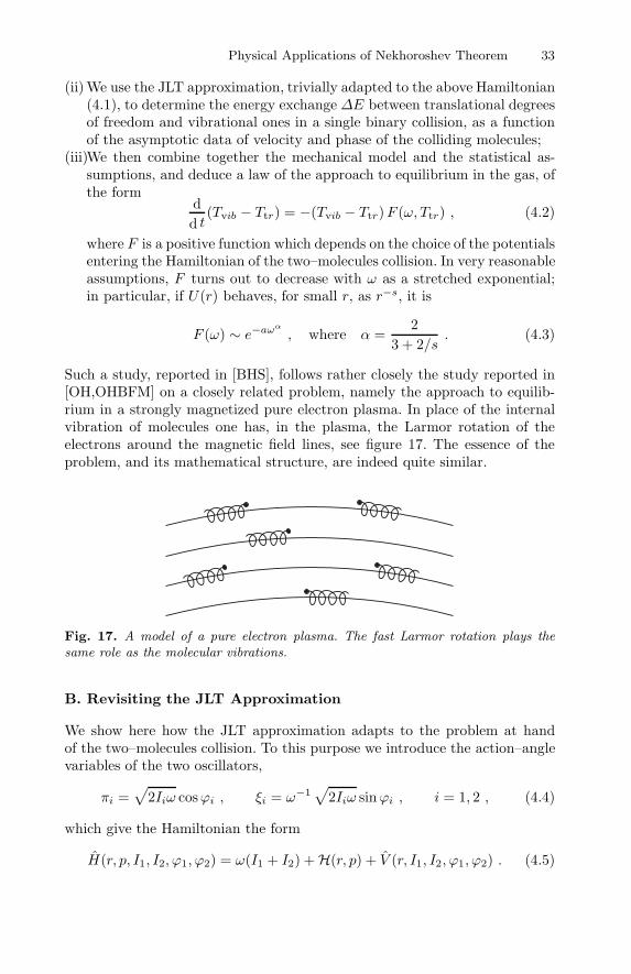
Physical Applications of Nekhoroshev Theorem 33
(ii) We use the JLT approximation, trivially adapted to the above Hamiltonian(4.1), to determine the energy exchange ∆E between translational degreesof freedom and vibrational ones in a single binary collision, as a functionof the asymptotic data of velocity and phase of the colliding molecules;
(iii)We then combine together the mechanical model and the statistical as-sumptions, and deduce a law of the approach to equilibrium in the gas, ofthe form
dd t
(Tvib − Ttr) = −(Tvib − Ttr)F (ω, Ttr) , (4.2)
where F is a positive function which depends on the choice of the potentialsentering the Hamiltonian of the two–molecules collision. In very reasonableassumptions, F turns out to decrease with ω as a stretched exponential;in particular, if U(r) behaves, for small r, as r−s, it is
F (ω) ∼ e−aωα
, where α =2
3 + 2/s. (4.3)
Such a study, reported in [BHS], follows rather closely the study reported in[OH,OHBFM] on a closely related problem, namely the approach to equilib-rium in a strongly magnetized pure electron plasma. In place of the internalvibration of molecules one has, in the plasma, the Larmor rotation of theelectrons around the magnetic field lines, see figure 17. The essence of theproblem, and its mathematical structure, are indeed quite similar.
Fig. 17. A model of a pure electron plasma. The fast Larmor rotation plays thesame role as the molecular vibrations.
B. Revisiting the JLT Approximation
We show here how the JLT approximation adapts to the problem at handof the two–molecules collision. To this purpose we introduce the action–anglevariables of the two oscillators,
πi =√
2Iiω cosϕi , ξi = ω−1√
2Iiω sinϕi , i = 1, 2 , (4.4)
which give the Hamiltonian the form
H(r, p, I1, I2, ϕ1, ϕ2) = ω(I1 + I2) +H(r, p) + V (r, I1, I2, ϕ1, ϕ2) . (4.5)
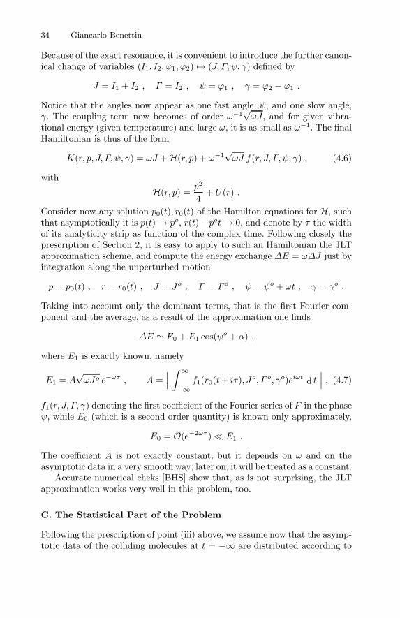
34 Giancarlo Benettin
Because of the exact resonance, it is convenient to introduce the further canon-ical change of variables (I1, I2, ϕ1, ϕ2) → (J, Γ, ψ, γ) defined by
J = I1 + I2 , Γ = I2 , ψ = ϕ1 , γ = ϕ2 − ϕ1 .
Notice that the angles now appear as one fast angle, ψ, and one slow angle,γ. The coupling term now becomes of order ω−1
√ωJ , and for given vibra-
tional energy (given temperature) and large ω, it is as small as ω−1. The finalHamiltonian is thus of the form
K(r, p, J, Γ, ψ, γ) = ωJ +H(r, p) + ω−1√ωJ f(r, J, Γ, ψ, γ) , (4.6)
with
H(r, p) =p2
4+ U(r) .
Consider now any solution p0(t), r0(t) of the Hamilton equations for H, suchthat asymptotically it is p(t)→ po, r(t)− pot→ 0, and denote by τ the widthof its analyticity strip as function of the complex time. Following closely theprescription of Section 2, it is easy to apply to such an Hamiltonian the JLTapproximation scheme, and compute the energy exchange ∆E = ω∆J just byintegration along the unperturbed motion
p = p0(t) , r = r0(t) , J = Jo , Γ = Γ o , ψ = ψo + ωt , γ = γo .
Taking into account only the dominant terms, that is the first Fourier com-ponent and the average, as a result of the approximation one finds
∆E E0 + E1 cos(ψo + α) ,
where E1 is exactly known, namely
E1 = A√ωJo e−ωτ , A =
∣∣∣
∫ ∞
−∞f1(r0(t+ iτ), Jo, Γ o, γo)eiωt d t
∣∣∣ , (4.7)
f1(r, J, Γ, γ) denoting the first coefficient of the Fourier series of F in the phaseψ, while E0 (which is a second order quantity) is known only approximately,
E0 = O(e−2ωτ ) E1 .
The coefficient A is not exactly constant, but it depends on ω and on theasymptotic data in a very smooth way; later on, it will be treated as a constant.
Accurate numerical cheks [BHS] show that, as is not surprising, the JLTapproximation works very well in this problem, too.
C. The Statistical Part of the Problem
Following the prescription of point (iii) above, we assume now that the asymp-totic data of the colliding molecules at t = −∞ are distributed according to
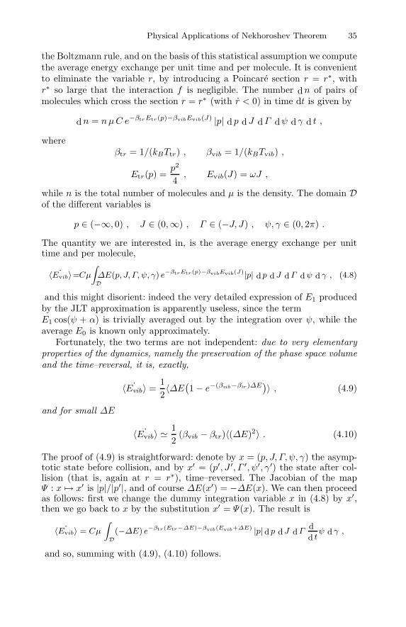
Physical Applications of Nekhoroshev Theorem 35
the Boltzmann rule, and on the basis of this statistical assumption we computethe average energy exchange per unit time and per molecule. It is convenientto eliminate the variable r, by introducing a Poincare section r = r∗, withr∗ so large that the interaction f is negligible. The number dn of pairs ofmolecules which cross the section r = r∗ (with r < 0) in time dt is given by
dn = nµC e−βtrEtr(p)−βvibEvib(J) |p| d p d J dΓ dψ d γ d t ,
whereβtr = 1/(kBTtr) , βvib = 1/(kBTvib) ,
Etr(p) =p2
4, Evib(J) = ωJ ,
while n is the total number of molecules and µ is the density. The domain Dof the different variables is
p ∈ (−∞, 0) , J ∈ (0,∞) , Γ ∈ (−J, J) , ψ, γ ∈ (0, 2π) .
The quantity we are interested in, is the average energy exchange per unittime and per molecule,
〈 ˙Evib〉=Cµ∫
D∆E(p, J, Γ, ψ, γ) e−βtrEtr(p)−βvibEvib(J)|p| d p d J dΓ dψ d γ , (4.8)
and this might disorient: indeed the very detailed expression of E1 producedby the JLT approximation is apparently useless, since the termE1 cos(ψ + α) is trivially averaged out by the integration over ψ, while theaverage E0 is known only approximately.
Fortunately, the two terms are not independent: due to very elementaryproperties of the dynamics, namely the preservation of the phase space volumeand the time–reversal, it is, exactly,
〈 ˙Evib〉 =12〈∆E
(
1− e−(βvib−βtr)∆E)
〉 , (4.9)
and for small ∆E
〈 ˙Evib〉 12
(βvib − βtr)〈(∆E)2〉 . (4.10)
The proof of (4.9) is straightforward: denote by x = (p, J, Γ, ψ, γ) the asymp-totic state before collision, and by x′ = (p′, J ′, Γ ′, ψ′, γ′) the state after col-lision (that is, again at r = r∗), time–reversed. The Jacobian of the mapΨ : x → x′ is |p|/|p′|, and of course ∆E(x′) = −∆E(x). We can then proceedas follows: first we change the dummy integration variable x in (4.8) by x′,then we go back to x by the substitution x′ = Ψ(x). The result is
〈 ˙Evib〉 = Cµ
∫
D(−∆E) e−βtr(Etr−∆E)−βvib(Evib+∆E) |p|d p dJ dΓ
d
d tψ d γ ,
and so, summing with (4.9), (4.10) follows.
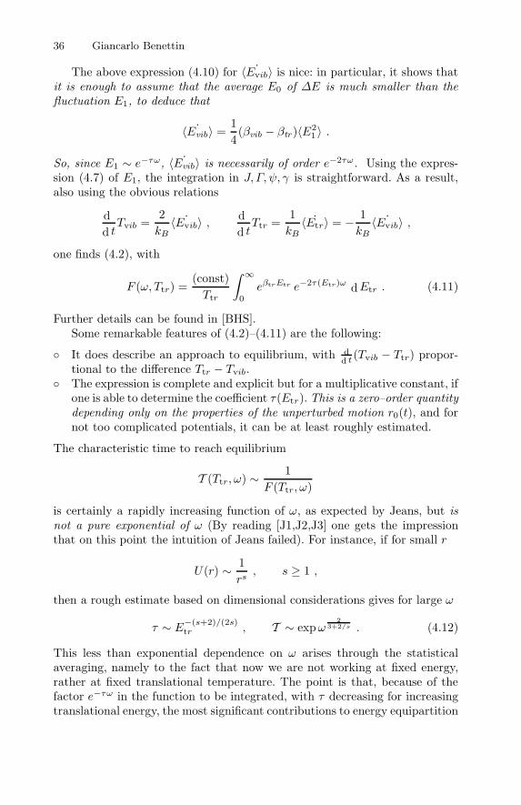
36 Giancarlo Benettin
The above expression (4.10) for 〈 ˙Evib〉 is nice: in particular, it shows thatit is enough to assume that the average E0 of ∆E is much smaller than thefluctuation E1, to deduce that
〈 ˙Evib〉 =14(βvib − βtr)〈E2
1 〉 .
So, since E1 ∼ e−τω, 〈 ˙Evib〉 is necessarily of order e−2τω. Using the expres-sion (4.7) of E1, the integration in J, Γ, ψ, γ is straightforward. As a result,also using the obvious relations
dd tTvib =
2kB〈 ˙Evib〉 ,
dd tTtr =
1kB〈Etr〉 = −
1kB〈 ˙Evib〉 ,
one finds (4.2), with
F (ω, Ttr) =(const)Ttr
∫ ∞
0
eβtrEtr e−2τ(Etr)ω dEtr . (4.11)
Further details can be found in [BHS].Some remarkable features of (4.2)–(4.11) are the following:
It does describe an approach to equilibrium, with dd t
(Tvib − Ttr) propor-tional to the difference Ttr − Tvib.
The expression is complete and explicit but for a multiplicative constant, ifone is able to determine the coefficient τ(Etr). This is a zero–order quantitydepending only on the properties of the unperturbed motion r0(t), and fornot too complicated potentials, it can be at least roughly estimated.
The characteristic time to reach equilibrium
T (Ttr, ω) ∼ 1F (Ttr, ω)
is certainly a rapidly increasing function of ω, as expected by Jeans, but isnot a pure exponential of ω (By reading [J1,J2,J3] one gets the impressionthat on this point the intuition of Jeans failed). For instance, if for small r
U(r) ∼ 1rs
, s ≥ 1 ,
then a rough estimate based on dimensional considerations gives for large ω
τ ∼ E−(s+2)/(2s)tr , T ∼ expω
23+2/s . (4.12)
This less than exponential dependence on ω arises through the statisticalaveraging, namely to the fact that now we are not working at fixed energy,rather at fixed translational temperature. The point is that, because of thefactor e−τω in the function to be integrated, with τ decreasing for increasingtranslational energy, the most significant contributions to energy equipartition
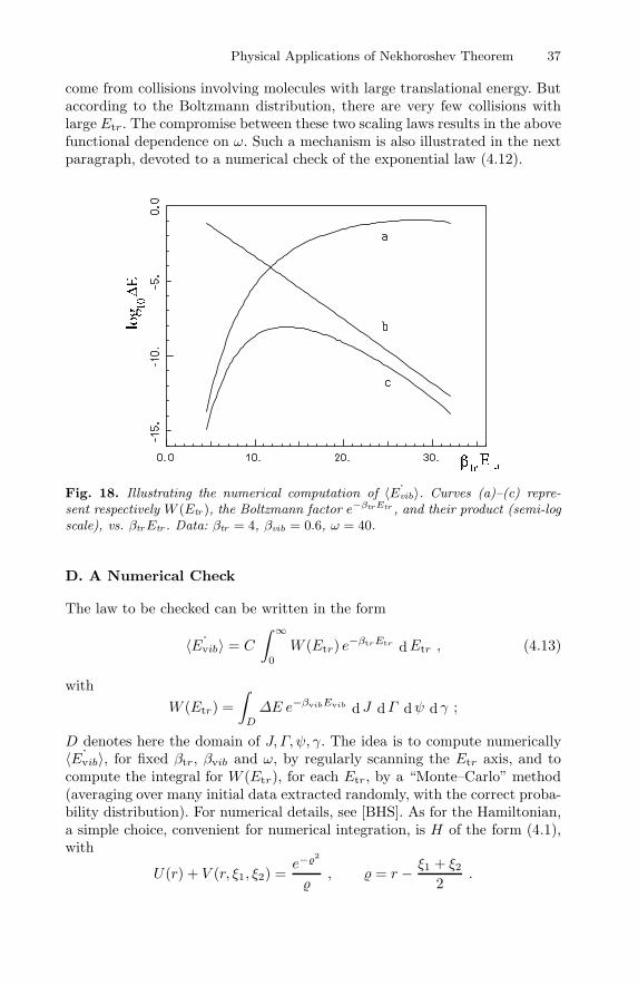
Physical Applications of Nekhoroshev Theorem 37
come from collisions involving molecules with large translational energy. Butaccording to the Boltzmann distribution, there are very few collisions withlarge Etr. The compromise between these two scaling laws results in the abovefunctional dependence on ω. Such a mechanism is also illustrated in the nextparagraph, devoted to a numerical check of the exponential law (4.12).
Fig. 18. Illustrating the numerical computation of 〈 ˙Evib〉. Curves (a)–(c) repre-sent respectively W (Etr), the Boltzmann factor e−βtrEtr , and their product (semi-logscale), vs. βtrEtr. Data: βtr = 4, βvib = 0.6, ω = 40.
D. A Numerical Check
The law to be checked can be written in the form
〈 ˙Evib〉 = C
∫ ∞
0
W (Etr) e−βtrEtr dEtr , (4.13)
withW (Etr) =
∫
D
∆E e−βvibEvib d J dΓ dψ d γ ;
D denotes here the domain of J, Γ, ψ, γ. The idea is to compute numerically〈 ˙Evib〉, for fixed βtr, βvib and ω, by regularly scanning the Etr axis, and tocompute the integral for W (Etr), for each Etr, by a “Monte–Carlo” method(averaging over many initial data extracted randomly, with the correct proba-bility distribution). For numerical details, see [BHS]. As for the Hamiltonian,a simple choice, convenient for numerical integration, is H of the form (4.1),with
U(r) + V (r, ξ1, ξ2) =e−
2
, = r − ξ1 + ξ2
2.
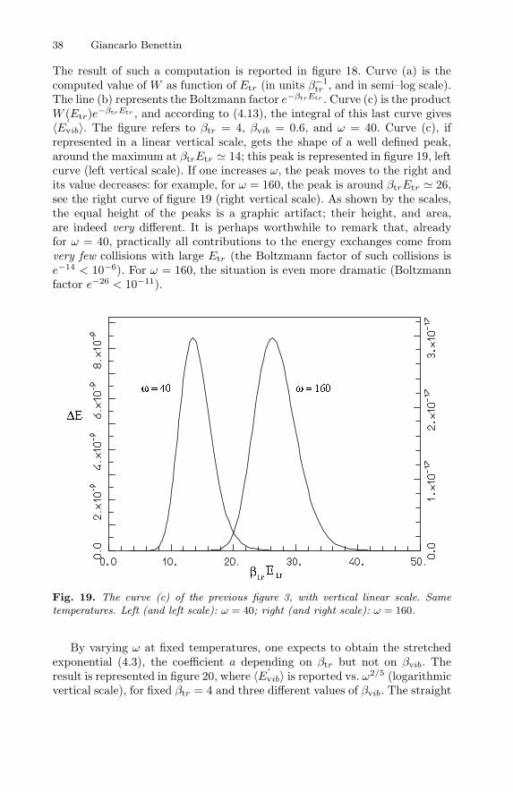
38 Giancarlo Benettin
The result of such a computation is reported in figure 18. Curve (a) is thecomputed value of W as function of Etr (in units β−1
tr , and in semi–log scale).The line (b) represents the Boltzmann factor e−βtrEtr . Curve (c) is the productW (Etr)e−βtrEtr , and according to (4.13), the integral of this last curve gives〈 ˙Evib〉. The figure refers to βtr = 4, βvib = 0.6, and ω = 40. Curve (c), ifrepresented in a linear vertical scale, gets the shape of a well defined peak,around the maximum at βtrEtr 14; this peak is represented in figure 19, leftcurve (left vertical scale). If one increases ω, the peak moves to the right andits value decreases: for example, for ω = 160, the peak is around βtrEtr 26,see the right curve of figure 19 (right vertical scale). As shown by the scales,the equal height of the peaks is a graphic artifact; their height, and area,are indeed very different. It is perhaps worthwhile to remark that, alreadyfor ω = 40, practically all contributions to the energy exchanges come fromvery few collisions with large Etr (the Boltzmann factor of such collisions ise−14 < 10−6). For ω = 160, the situation is even more dramatic (Boltzmannfactor e−26 < 10−11).
Fig. 19. The curve (c) of the previous figure 3, with vertical linear scale. Sametemperatures. Left (and left scale): ω = 40; right (and right scale): ω = 160.
By varying ω at fixed temperatures, one expects to obtain the stretchedexponential (4.3), the coefficient a depending on βtr but not on βvib. Theresult is represented in figure 20, where 〈 ˙Evib〉 is reported vs. ω2/5 (logarithmicvertical scale), for fixed βtr = 4 and three different values of βvib. The straight
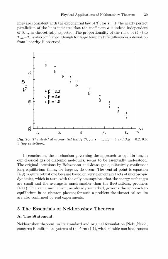
Physical Applications of Nekhoroshev Theorem 39
lines are consistent with the exponential law (4.3), for s = 1; the nearly perfectparallelism of the lines indicates that the coefficient a is indeed independentof βvib, as theoretically expected. The proportionality of the r.h.s. of (4.3) toTvib−Tt is also confirmed, though for large temperature differences a deviationfrom linearity is observed.
Fig. 20. The stretched exponential law (4.3), for s = 1; βtr = 4 and βvib = 0.2, 0.6,1 (top to bottom).
In conclusion, the mechanism governing the approach to equilibrium, inour classical gas of diatomic molecules, seems to be essentially understood.The original intuitions by Boltzmann and Jeans get qualitatively confirmed:long equilibrium times, for large ω, do occur. The central point is equation(4.9), a quite robust one because based on very elementary facts of microscopicdynamics, which in turn, with the only assumptions that the energy exchangesare small and the average is much smaller than the fluctuations, produces(4.11). The same mechanism, as already remarked, governs the approach toequilibrium in an electron plasma; for such a problem the theoretical resultsare also confirmed by real experiments.
5 The Essentials of Nekhoroshev Theorem
A. The Statement
Nekhoroshev theorem, in its standard and original formulation [Nek1,Nek2],concerns Hamiltonian systems of the form (1.1), with suitable non isochronous
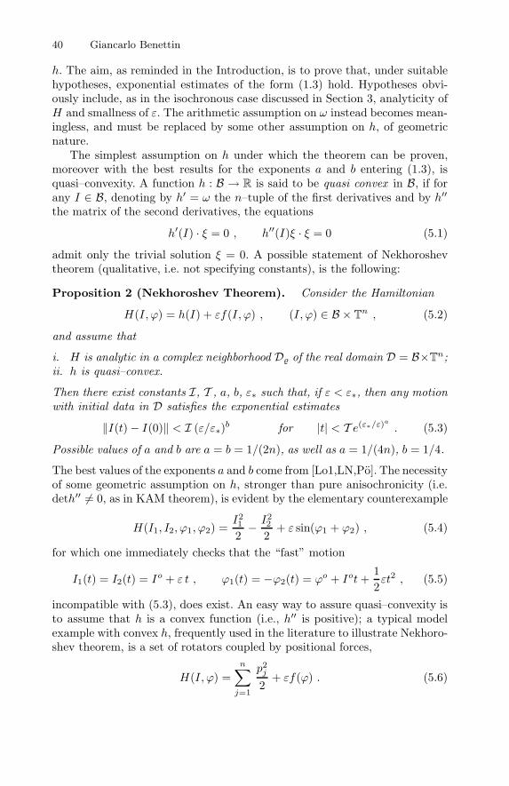
40 Giancarlo Benettin
h. The aim, as reminded in the Introduction, is to prove that, under suitablehypotheses, exponential estimates of the form (1.3) hold. Hypotheses obvi-ously include, as in the isochronous case discussed in Section 3, analyticity ofH and smallness of ε. The arithmetic assumption on ω instead becomes mean-ingless, and must be replaced by some other assumption on h, of geometricnature.
The simplest assumption on h under which the theorem can be proven,moreover with the best results for the exponents a and b entering (1.3), isquasi–convexity. A function h : B → R is said to be quasi convex in B, if forany I ∈ B, denoting by h′ = ω the n–tuple of the first derivatives and by h′′
the matrix of the second derivatives, the equations
h′(I) · ξ = 0 , h′′(I)ξ · ξ = 0 (5.1)
admit only the trivial solution ξ = 0. A possible statement of Nekhoroshevtheorem (qualitative, i.e. not specifying constants), is the following:
Proposition 2 (Nekhoroshev Theorem). Consider the Hamiltonian
H(I, ϕ) = h(I) + εf(I, ϕ) , (I, ϕ) ∈ B × Tn , (5.2)
and assume that
i. H is analytic in a complex neighborhood D of the real domain D = B×Tn;
ii. h is quasi–convex.
Then there exist constants I, T , a, b, ε∗ such that, if ε < ε∗, then any motionwith initial data in D satisfies the exponential estimates
‖I(t)− I(0)‖ < I (ε/ε∗)b for |t| < T e(ε∗/ε)a
. (5.3)
Possible values of a and b are a = b = 1/(2n), as well as a = 1/(4n), b = 1/4.
The best values of the exponents a and b come from [Lo1,LN,Po]. The necessityof some geometric assumption on h, stronger than pure anisochronicity (i.e.deth′′ = 0, as in KAM theorem), is evident by the elementary counterexample
H(I1, I2, ϕ1, ϕ2) =I21
2− I2
2
2+ ε sin(ϕ1 + ϕ2) , (5.4)
for which one immediately checks that the “fast” motion
I1(t) = I2(t) = Io + ε t , ϕ1(t) = −ϕ2(t) = ϕo + Iot+12εt2 , (5.5)
incompatible with (5.3), does exist. An easy way to assure quasi–convexity isto assume that h is a convex function (i.e., h′′ is positive); a typical modelexample with convex h, frequently used in the literature to illustrate Nekhoro-shev theorem, is a set of rotators coupled by positional forces,
H(I, ϕ) =n∑
j=1
p2j
2+ εf(ϕ) . (5.6)
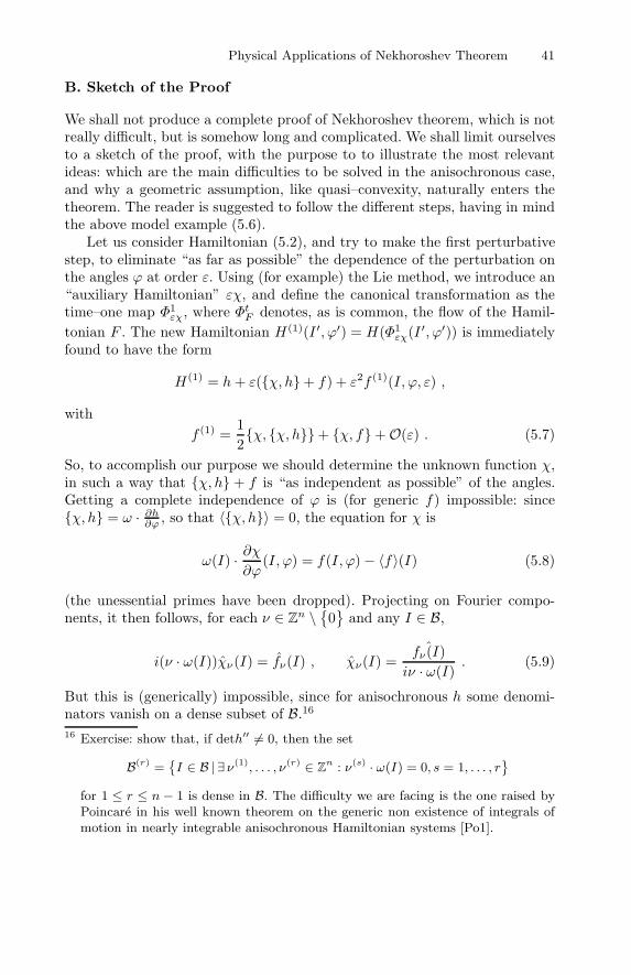
Physical Applications of Nekhoroshev Theorem 41
B. Sketch of the Proof
We shall not produce a complete proof of Nekhoroshev theorem, which is notreally difficult, but is somehow long and complicated. We shall limit ourselvesto a sketch of the proof, with the purpose to to illustrate the most relevantideas: which are the main difficulties to be solved in the anisochronous case,and why a geometric assumption, like quasi–convexity, naturally enters thetheorem. The reader is suggested to follow the different steps, having in mindthe above model example (5.6).
Let us consider Hamiltonian (5.2), and try to make the first perturbativestep, to eliminate “as far as possible” the dependence of the perturbation onthe angles ϕ at order ε. Using (for example) the Lie method, we introduce an“auxiliary Hamiltonian” εχ, and define the canonical transformation as thetime–one map Φ1
εχ, where ΦtF denotes, as is common, the flow of the Hamil-tonian F . The new Hamiltonian H(1)(I ′, ϕ′) = H(Φ1
εχ(I ′, ϕ′)) is immediatelyfound to have the form
H(1) = h+ ε(χ, h+ f) + ε2f (1)(I, ϕ, ε) ,
withf (1) =
12χ, χ, h+ χ, f+O(ε) . (5.7)
So, to accomplish our purpose we should determine the unknown function χ,in such a way that χ, h + f is “as independent as possible” of the angles.Getting a complete independence of ϕ is (for generic f) impossible: sinceχ, h = ω · ∂h∂ϕ , so that 〈χ, h〉 = 0, the equation for χ is
ω(I) · ∂χ∂ϕ
(I, ϕ) = f(I, ϕ)− 〈f〉(I) (5.8)
(the unessential primes have been dropped). Projecting on Fourier compo-nents, it then follows, for each ν ∈ Z
n \
0
and any I ∈ B,
i(ν · ω(I))χν(I) = fν(I) , χν(I) =ˆfν(I)
iν · ω(I). (5.9)
But this is (generically) impossible, since for anisochronous h some denomi-nators vanish on a dense subset of B.16
16 Exercise: show that, if deth′′ = 0, then the set
B(r) =
I ∈ B | ∃ ν(1), . . . , ν(r) ∈ Zn : ν(s) · ω(I) = 0, s = 1, . . . , r
for 1 ≤ r ≤ n− 1 is dense in B. The difficulty we are facing is the one raised byPoincare in his well known theorem on the generic non existence of integrals ofmotion in nearly integrable anisochronous Hamiltonian systems [Po1].
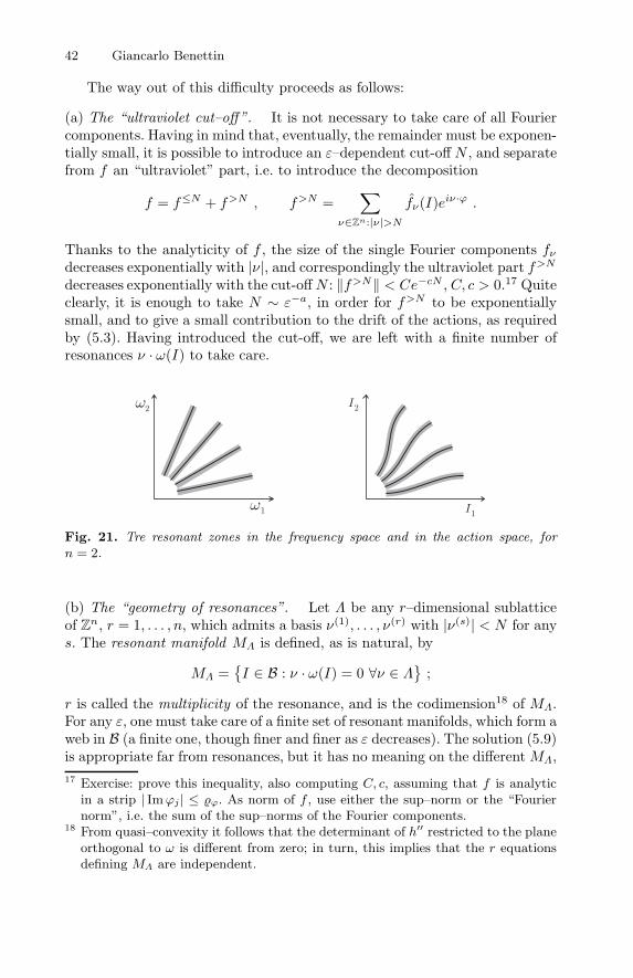
42 Giancarlo Benettin
The way out of this difficulty proceeds as follows:
(a) The “ultraviolet cut–off”. It is not necessary to take care of all Fouriercomponents. Having in mind that, eventually, the remainder must be exponen-tially small, it is possible to introduce an ε–dependent cut-off N , and separatefrom f an “ultraviolet” part, i.e. to introduce the decomposition
f = f≤N + f>N , f>N =∑
ν∈Zn:|ν|>Nfν(I)eiν·ϕ .
Thanks to the analyticity of f , the size of the single Fourier components fνdecreases exponentially with |ν|, and correspondingly the ultraviolet part f>N
decreases exponentially with the cut-offN : ‖f>N‖ < Ce−cN , C, c > 0.17 Quiteclearly, it is enough to take N ∼ ε−a, in order for f>N to be exponentiallysmall, and to give a small contribution to the drift of the actions, as requiredby (5.3). Having introduced the cut-off, we are left with a finite number ofresonances ν · ω(I) to take care.
Fig. 21. Tre resonant zones in the frequency space and in the action space, forn = 2.
(b) The “geometry of resonances”. Let Λ be any r–dimensional sublatticeof Z
n, r = 1, . . . , n, which admits a basis ν(1), . . . , ν(r) with |ν(s)| < N for anys. The resonant manifold MΛ is defined, as is natural, by
MΛ =
I ∈ B : ν · ω(I) = 0 ∀ν ∈ Λ
;
r is called the multiplicity of the resonance, and is the codimension18 of MΛ.For any ε, one must take care of a finite set of resonant manifolds, which form aweb in B (a finite one, though finer and finer as ε decreases). The solution (5.9)is appropriate far from resonances, but it has no meaning on the different MΛ,17 Exercise: prove this inequality, also computing C, c, assuming that f is analytic
in a strip | Imϕj | ≤ ϕ. As norm of f , use either the sup–norm or the “Fouriernorm”, i.e. the sum of the sup–norms of the Fourier components.
18 From quasi–convexity it follows that the determinant of h′′ restricted to the planeorthogonal to ω is different from zero; in turn, this implies that the r equationsdefining MΛ are independent.
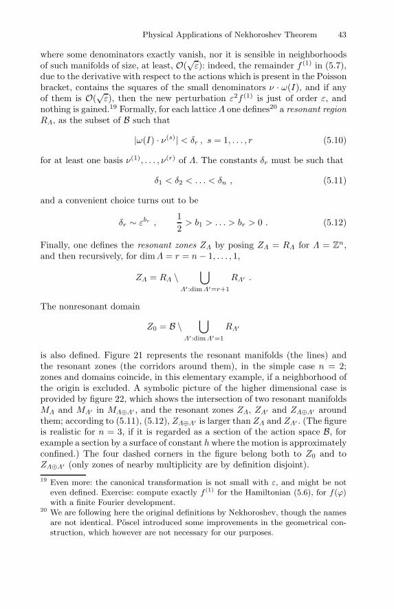
Physical Applications of Nekhoroshev Theorem 43
where some denominators exactly vanish, nor it is sensible in neighborhoodsof such manifolds of size, at least, O(
√ε): indeed, the remainder f (1) in (5.7),
due to the derivative with respect to the actions which is present in the Poissonbracket, contains the squares of the small denominators ν · ω(I), and if anyof them is O(
√ε), then the new perturbation ε2f (1) is just of order ε, and
nothing is gained.19 Formally, for each lattice Λ one defines20 a resonant regionRΛ, as the subset of B such that
|ω(I) · ν(s)| < δr , s = 1, . . . , r (5.10)
for at least one basis ν(1), . . . , ν(r) of Λ. The constants δr must be such that
δ1 < δ2 < . . . < δn , (5.11)
and a convenient choice turns out to be
δr ∼ εbr ,12> b1 > . . . > br > 0 . (5.12)
Finally, one defines the resonant zones ZΛ by posing ZΛ = RΛ for Λ = Zn,
and then recursively, for dimΛ = r = n− 1, . . . , 1,
ZΛ = RΛ \⋃
Λ′:dimΛ′=r+1
RΛ′ .
The nonresonant domain
Z0 = B \⋃
Λ′:dimΛ′=1
RΛ′
is also defined. Figure 21 represents the resonant manifolds (the lines) andthe resonant zones (the corridors around them), in the simple case n = 2;zones and domains coincide, in this elementary example, if a neighborhood ofthe origin is excluded. A symbolic picture of the higher dimensional case isprovided by figure 22, which shows the intersection of two resonant manifoldsMΛ and MΛ′ in MΛ⊕Λ′ , and the resonant zones ZΛ, ZΛ′ and ZΛ⊕Λ′ aroundthem; according to (5.11), (5.12), ZΛ⊕Λ′ is larger than ZΛ and ZΛ′ . (The figureis realistic for n = 3, if it is regarded as a section of the action space B, forexample a section by a surface of constant h where the motion is approximatelyconfined.) The four dashed corners in the figure belong both to Z0 and toZΛ⊕Λ′ (only zones of nearby multiplicity are by definition disjoint).
19 Even more: the canonical transformation is not small with ε, and might be noteven defined. Exercise: compute exactly f (1) for the Hamiltonian (5.6), for f(ϕ)with a finite Fourier development.
20 We are following here the original definitions by Nekhoroshev, though the namesare not identical. Poscel introduced some improvements in the geometrical con-struction, which however are not necessary for our purposes.
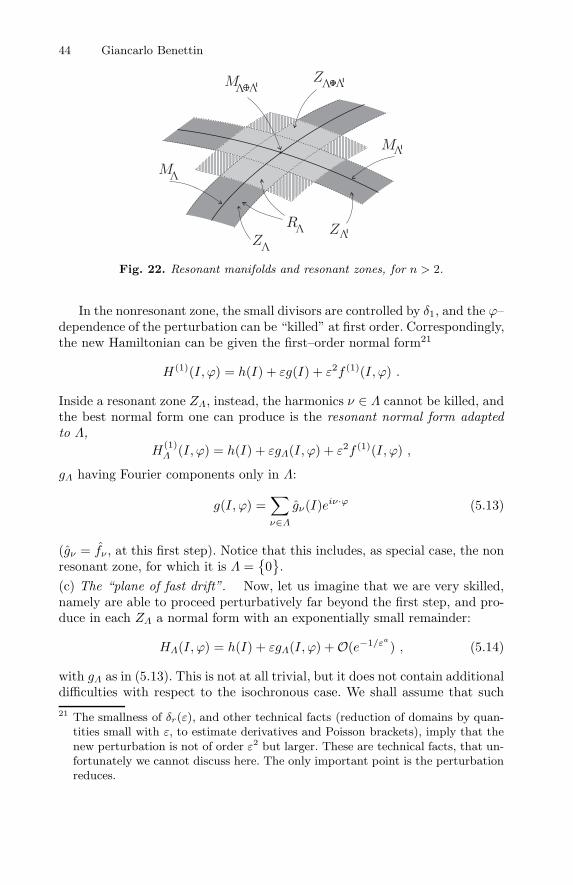
44 Giancarlo Benettin
Fig. 22. Resonant manifolds and resonant zones, for n > 2.
In the nonresonant zone, the small divisors are controlled by δ1, and the ϕ–dependence of the perturbation can be “killed” at first order. Correspondingly,the new Hamiltonian can be given the first–order normal form21
H(1)(I, ϕ) = h(I) + εg(I) + ε2f (1)(I, ϕ) .
Inside a resonant zone ZΛ, instead, the harmonics ν ∈ Λ cannot be killed, andthe best normal form one can produce is the resonant normal form adaptedto Λ,
H(1)Λ (I, ϕ) = h(I) + εgΛ(I, ϕ) + ε2f (1)(I, ϕ) ,
gΛ having Fourier components only in Λ:
g(I, ϕ) =∑
ν∈Λgν(I)eiν·ϕ (5.13)
(gν = fν , at this first step). Notice that this includes, as special case, the nonresonant zone, for which it is Λ =
0
.(c) The “plane of fast drift”. Now, let us imagine that we are very skilled,namely are able to proceed perturbatively far beyond the first step, and pro-duce in each ZΛ a normal form with an exponentially small remainder:
HΛ(I, ϕ) = h(I) + εgΛ(I, ϕ) +O(e−1/εa
) , (5.14)
with gΛ as in (5.13). This is not at all trivial, but it does not contain additionaldifficulties with respect to the isochronous case. We shall assume that such21 The smallness of δr(ε), and other technical facts (reduction of domains by quan-
tities small with ε, to estimate derivatives and Poisson brackets), imply that thenew perturbation is not of order ε2 but larger. These are technical facts, that un-fortunately we cannot discuss here. The only important point is the perturbationreduces.
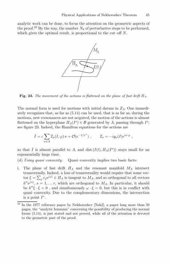
Physical Applications of Nekhoroshev Theorem 45
analytic work can be done, to focus the attention on the geometric aspects ofthe proof.22 By the way, the number N0 of perturbative steps to be performed,which gives the optimal result, is proportional to the cut–off N .
Fig. 23. The movement of the actions is flattened on the plane of fast drift ΠΛ.
The normal form is used for motions with initial datum in ZΛ. One immedi-ately recognizes that, as far as (5.14) can be used, that is as far as, during themotions, new rresonances are not acquired, the motion of the actions is almostflattened on the hyperplane ΠΛ(Io) ∈ B generated by Λ, passing through Io;see figure 23. Indeed, the Hamilton equations for the actions are
I = ε∑
ν∈ΛIν(I, ϕ) ν +O(e−1/εa
) , Iν = −igν(I)eiν·ϕ ,
so that I is almost parallel to Λ, and dist (I(t), ΠΛ(Io)) stays small for anexponentially large time.(d) Using quasi–convexity. Quasi–convexity implies two basic facts:
i. The plane of fast drift ΠΛ and the resonant manifold MΛ intersecttransversally. Indeed, a loss of transversality would require that some vec-tor ξ =
∑
j cjν(j) ∈ ΠΛ is tangent to MΛ, and so orthogonal to all vectors
h′′ν(s), s = 1, . . . r, which are orthogonal to MΛ. In particular, it shouldbe h′′ξ · ξ = 0 , and simultaneously ω · ξ = 0, but this is in conflict withquasi–convexity. Due to the complementary dimensions, the intersectionis a point I∗.
22 In the 1977 reference paper by Nekhoroshev [Nek2], a paper long more than 50pages, the “analytic lemmma” concerning the possibility of producing the normalforms (5.14), is just stated and not proved, while all of the attention is devotedto the geometric part of the proof.
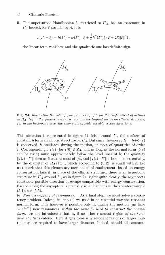
46 Giancarlo Benettin
ii. The unperturbed Hamiltonian h, restricted to ΠΛ, has an extremum inI∗. Indeed, for ξ parallel to Λ, it is
h(I∗ + ξ) = h(I∗) + ω(I∗) · ξ +12h′′(I∗)ξ · ξ +O(‖ξ‖3) ;
the linear term vanishes, and the quadratic one has definite sign.
Fig. 24. Illustrating the role of quasi–convexity of h for the confinement of actionsin ΠΛ: (a) in the quasi–convex case, actions are trapped inside an elliptic structure;(b) in the hyperbolic case, the asymptots provide possible escape directions.
This situation is represented in figure 24, left: around I∗, the surfaces ofconstant h form an elliptic structure onΠΛ. But since the energyH = h+O(ε)is conserved, h oscillates, during the motion, at most of quantities of orderε. Correspondingly I(t) (for I(0) ∈ ZΛ, and as long as the normal form (5.8)can be used) must approximately follow the level lines of h; the quantity‖I(t)−I∗‖ then oscillates at most of
√ε, and ‖I(t)−Io‖ is bounded, essentially,
by the diameter of ΠΛ ∩ ZΛ, which according to (5.12) is small with ε. Letus remark that this elementary mechanism of confinement, based on energyconservation, fails if, in place of the elliptic structure, there is an hyperbolicstructure in ΠΛ around I∗, as in figure 24, right: quite clearly, the asymptotsconstitute possible direction of escape compatible with energy conservation.Escape along the asymptots is precisely what happens in the counterexample(5.4), see (5.5).(e) Non overlapping of resonances. As a final step, we must solve a consis-tency problem. Indeed, in step (c) we used in an essential way the resonantnormal form. This however is possible only if, during the motion (up time∼ e1/ε
a
) new resonances, within the same δr used to construct the normalform, are not introduced: that is, if no other resonant region of the samemultiplicity is entered. Here it gets clear why resonant regions of larger mul-tiplicity are required to have larger diameter. Indeed, should all constants
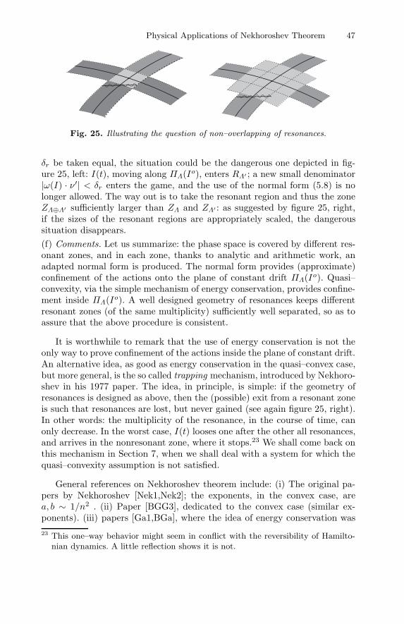
Physical Applications of Nekhoroshev Theorem 47
Fig. 25. Illustrating the question of non–overlapping of resonances.
δr be taken equal, the situation could be the dangerous one depicted in fig-ure 25, left: I(t), moving along ΠΛ(Io), enters RΛ′ ; a new small denominator|ω(I) · ν′| < δr enters the game, and the use of the normal form (5.8) is nolonger allowed. The way out is to take the resonant region and thus the zoneZΛ⊕Λ′ sufficiently larger than ZΛ and ZΛ′ : as suggested by figure 25, right,if the sizes of the resonant regions are appropriately scaled, the dangeroussituation disappears.(f) Comments. Let us summarize: the phase space is covered by different res-onant zones, and in each zone, thanks to analytic and arithmetic work, anadapted normal form is produced. The normal form provides (approximate)confinement of the actions onto the plane of constant drift ΠΛ(Io). Quasi–convexity, via the simple mechanism of energy conservation, provides confine-ment inside ΠΛ(Io). A well designed geometry of resonances keeps differentresonant zones (of the same multiplicity) sufficiently well separated, so as toassure that the above procedure is consistent.
It is worthwhile to remark that the use of energy conservation is not theonly way to prove confinement of the actions inside the plane of constant drift.An alternative idea, as good as energy conservation in the quasi–convex case,but more general, is the so called trapping mechanism, introduced by Nekhoro-shev in his 1977 paper. The idea, in principle, is simple: if the geometry ofresonances is designed as above, then the (possible) exit from a resonant zoneis such that resonances are lost, but never gained (see again figure 25, right).In other words: the multiplicity of the resonance, in the course of time, canonly decrease. In the worst case, I(t) looses one after the other all resonances,and arrives in the nonresonant zone, where it stops.23 We shall come back onthis mechanism in Section 7, when we shall deal with a system for which thequasi–convexity assumption is not satisfied.
General references on Nekhoroshev theorem include: (i) The original pa-pers by Nekhoroshev [Nek1,Nek2]; the exponents, in the convex case, area, b ∼ 1/n2 . (ii) Paper [BGG3], dedicated to the convex case (similar ex-ponents). (iii) papers [Ga1,BGa], where the idea of energy conservation was
23 This one–way behavior might seem in conflict with the reversibility of Hamilto-nian dynamics. A little reflection shows it is not.
48 Giancarlo Benettin
first fully exploited; possible exponents include a = 1/8, b ∼ 1/n2. (iv) papers[Lo1,LN], very interesting both for the result, namely a = b = 1/(2n) (a muchlonger time scale), and for a revolutionary technique.24 (v) paper [Po1], wherethe geometry of resonances was improved; the result is a = b = 1/(2n), as wellas a = 1/2, b = 1/(4n). Other papers concern applications and extensions tospecial systems, including systems with infinitely many degrees of freedom.
C. Pathologies in Physical Systems
According to the purpose outlined in the Introduction, we shall now focusthe attention to physical applications of Nekhoroshev theorem. Applications,however, are far from trivial, since most interesting systems to which onewould like to apply the theorem, do not fit the assumptions. Two pathologiestypically occur:
i. The integrable system is properly degenerate, namely the numberm of con-stants of motion exceeds the number n of degrees of freedom. Well knownexamples are the Euler–Poinsot rigid body (the rigid body with a fixedpoint, in absence of external torques), for which n = 3 and m = 4, and theKepler system, for which n = 3 and m = 5. The result of degeneracy isthat the number of actions effectively entering the unperturbed Hamilto-nian h is n0 = 2n−m < n, and quasi–convexity (as well as steepness, seelater) is violated. Using the notation I, ϕ for the actions effectively presentin the unperturbed Hamiltonian and their conjugated angles, and p, q forthe remaining variables, the perturbed Hamiltonian has the form
H(I, ϕ, p, q) = h(I) + εf(I, ϕ, p, q) .
For such a system, using the standard techniques of perturbation theory,it is not difficult to produce resonant or nonresonant normal forms, up toan exponentially small ϕ–dependent remainder, say
HΛ(I, ϕ, p, q) = h(I) + εgΛ(I, ϕ, p, q) +O(e−1/εa
)gΛ(I, ϕ, p, q) =
∑
ν∈Λ gν(I, p, q)eiν·ϕ ,
so as to keep control of I1, . . . , In0 (in case of convex h). But this is apoor result, for two reasons: first of all, the p, q variables are typically veryinteresting (for the rigid body, they determine the spatial orientation of theangular momentum; for the Kepler problem, they include the eccentricityand inclination of the Keplerian ellipsis). Moreover, these variables couldapproach a singularity in a short time: the normal form gets then useless,and long time stability of the actions cannot be deduced.
24 The geometric part, in particular, is highly semplified, since only resonances ofmultiplicity n − 1 are considered. A quick easier proof, unfortunately strictlylimited to the convex case.
Physical Applications of Nekhoroshev Theorem 49
ii. The action–angle coordinates get singular somewhere in the phase space,often in correspondence to the most interesting motions. Examples in-clude the proper rotations of the rigid body around a symmetry axis, thecircular orbits of the Kepler problem, and a set of harmonic oscillatorswhenever any of them is at rest. From a geometric point of view, singularmotions are motions on singular lower dimensional leaves of the foliationinto invariant tori: an n–dimensional torus (n0–dimensional, for degener-ate systems) shrinks to a lower dimensional one, and correspondingly anangle gets undefined (the angle giving the orientation of the pericenter,for the Keplerian ellipses; the angle giving the precession of the symmetryaxis of the body around the direction of the angular momentum, for therigid body; the phase of the oscillator at rest, in the last example). Thequestion to be solved (more technical, but not completely technical) is howto proceed perturbatively without using the action–angle variables.
Both difficulties are present in the examples that we are going to study in theremaining part of these lectures.
6 The Perturbed Euler–Poinsot Rigid Body
The Euler–Poinsot rigid body is a rigid body with a fixed point, in absence ofexternal torques. We shall restrict ourselves to the symmetric case, i.e. whentwo inertia moments are equal, though most results could be adapted to thetriaxial case. Before entering the perturbative study, we must shortly reviewfrom a geometric point of view the behaviour of the unperturbed system.
A. The Unperturbed System
Let (ex, ey, ez) be a basis fixed in the space, and (e1, e2, e3) be a proper basisof the body, with inertia moments A1 = A2 = A3. The phase space of thesystem is the cotangent boundle M = T ∗SO(3), which however is trivialand can be identified with SO(3) × R
3. A point of M is identified by a pair(R,M), where R ∈ SO(3) is the matrix such that Rex = e1 and so on,while M = (Mx,My,Mz) ∈ R
3 is the angular momentum in the space.25
Alternatively, one can use m = (m1,m2,m3) = R−1M (the so–called bodyrepresentation of the angular momentum) in place of M ; the pair (R,m) alsoprovides a good parametrization of T ∗
RSO(3).The Euler–Poinsot rigid body has four independent integrals of motion. A
possible choice is given by25 The triviality of T ∗SO(3) precisely expresses the fact that the angular momentumM exists, as vector in R
3, regardless of the configuration R of the body. In a similarway, the triviality of the tangent bundle TSO(3) expresses geometrically the wellknown existence of the angular velocity as a vector of R
3.
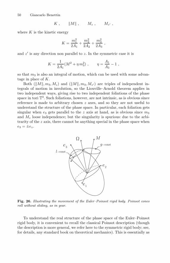
50 Giancarlo Benettin
K , ‖M‖ , Mz , Mz′ ,
where K is the kinetic energy
K =m2
1
2A1+m2
2
2A2+m2
3
2A3,
and z′ is any direction non parallel to z. In the symmetric case it is
K =1
2A1(M2 + ηm2
3) , η =A1
A3− 1 ,
so that m3 is also an integral of motion, which can be used with some advan-tage in place of K.
Both (‖M‖,m3,Mz) and (‖M‖,m3,Mz′) are triples of independent in-tegrals of motion in involution, so the Liouville–Arnold theorem applies intwo independent ways, giving rise to two independent foliations of the phasespace in tori T
3. Such foliations, however, are not intrinsic, as is obvious sincereference is made to arbitrary chosen z axes, and so they are not useful tounderstand the structure of the phase space. In particular, each foliation getssingular when e3 gets parallel to the z axis at hand, as is obvious since m3
and Mz loose independence; but the singularity is spurious: due to the arbi-trarity of the z axis, there cannot be anything special in the phase space whene3 = ±ez.
Fig. 26. Illustrating the movement of the Euler–Poinsot rigid body. Poinsot conesroll without sliding, as in gear.
To understand the real structure of the phase space of the Euler–Poinsotrigid body, it is convenient to recall the classical Poinsot description (thoughthe description is more general, we refer here to the symmetric rigid body; see,for details, any standard book on theoretical mechanics). This is essentially as
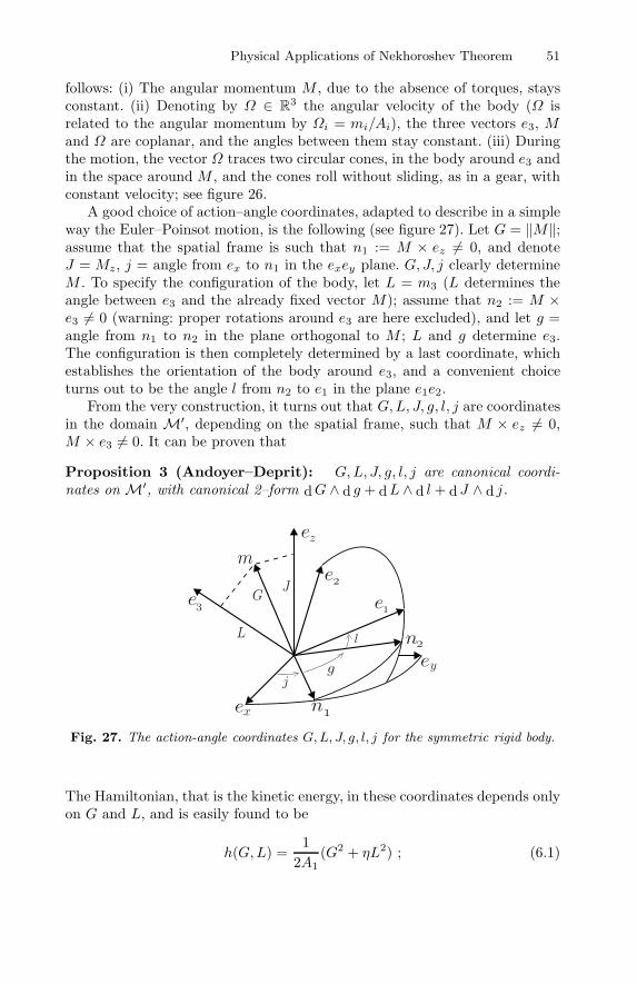
Physical Applications of Nekhoroshev Theorem 51
follows: (i) The angular momentum M , due to the absence of torques, staysconstant. (ii) Denoting by Ω ∈ R
3 the angular velocity of the body (Ω isrelated to the angular momentum by Ωi = mi/Ai), the three vectors e3, Mand Ω are coplanar, and the angles between them stay constant. (iii) Duringthe motion, the vector Ω traces two circular cones, in the body around e3 andin the space around M , and the cones roll without sliding, as in a gear, withconstant velocity; see figure 26.
A good choice of action–angle coordinates, adapted to describe in a simpleway the Euler–Poinsot motion, is the following (see figure 27). Let G = ‖M‖;assume that the spatial frame is such that n1 := M × ez = 0, and denoteJ = Mz, j = angle from ex to n1 in the exey plane. G, J, j clearly determineM . To specify the configuration of the body, let L = m3 (L determines theangle between e3 and the already fixed vector M); assume that n2 := M ×e3 = 0 (warning: proper rotations around e3 are here excluded), and let g =angle from n1 to n2 in the plane orthogonal to M ; L and g determine e3.The configuration is then completely determined by a last coordinate, whichestablishes the orientation of the body around e3, and a convenient choiceturns out to be the angle l from n2 to e1 in the plane e1e2.
From the very construction, it turns out that G,L, J, g, l, j are coordinatesin the domain M′, depending on the spatial frame, such that M × ez = 0,M × e3 = 0. It can be proven that
Proposition 3 (Andoyer–Deprit): G,L, J, g, l, j are canonical coordi-nates on M′, with canonical 2–form dG ∧ d g + dL ∧ d l + d J ∧ d j.
Fig. 27. The action-angle coordinates G,L, J, g, l, j for the symmetric rigid body.
The Hamiltonian, that is the kinetic energy, in these coordinates depends onlyon G and L, and is easily found to be
h(G,L) =1
2A1(G2 + ηL2) ; (6.1)
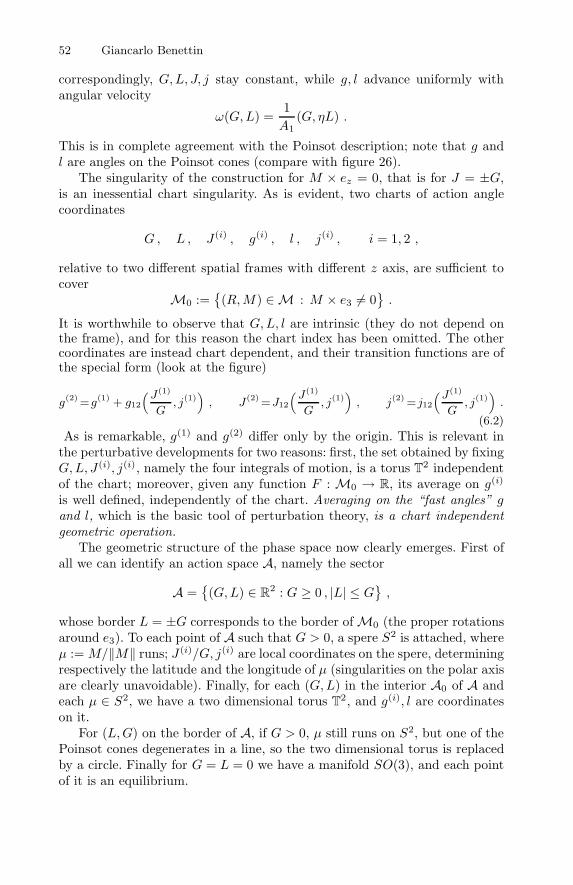
52 Giancarlo Benettin
correspondingly, G,L, J, j stay constant, while g, l advance uniformly withangular velocity
ω(G,L) =1A1
(G, ηL) .
This is in complete agreement with the Poinsot description; note that g andl are angles on the Poinsot cones (compare with figure 26).
The singularity of the construction for M × ez = 0, that is for J = ±G,is an inessential chart singularity. As is evident, two charts of action anglecoordinates
G , L , J (i) , g(i) , l , j(i) , i = 1, 2 ,
relative to two different spatial frames with different z axis, are sufficient tocover
M0 :=
(R,M) ∈M : M × e3 = 0
.
It is worthwhile to observe that G,L, l are intrinsic (they do not depend onthe frame), and for this reason the chart index has been omitted. The othercoordinates are instead chart dependent, and their transition functions are ofthe special form (look at the figure)
g(2) =g(1) + g12(J(1)
G, j(1)
)
, J(2) =J12
(J(1)
G, j(1)
)
, j(2) =j12(J(1)
G, j(1)
)
.
(6.2)
As is remarkable, g(1) and g(2) differ only by the origin. This is relevant inthe perturbative developments for two reasons: first, the set obtained by fixingG,L, J (i), j(i), namely the four integrals of motion, is a torus T
2 independentof the chart; moreover, given any function F : M0 → R, its average on g(i)
is well defined, independently of the chart. Averaging on the “fast angles” gand l, which is the basic tool of perturbation theory, is a chart independentgeometric operation.
The geometric structure of the phase space now clearly emerges. First ofall we can identify an action space A, namely the sector
A =
(G,L) ∈ R2 : G ≥ 0 , |L| ≤ G
,
whose border L = ±G corresponds to the border ofM0 (the proper rotationsaround e3). To each point of A such that G > 0, a spere S2 is attached, whereµ := M/‖M‖ runs; J (i)/G, j(i) are local coordinates on the spere, determiningrespectively the latitude and the longitude of µ (singularities on the polar axisare clearly unavoidable). Finally, for each (G,L) in the interior A0 of A andeach µ ∈ S2, we have a two dimensional torus T
2, and g(i), l are coordinateson it.
For (L,G) on the border of A, if G > 0, µ still runs on S2, but one of thePoinsot cones degenerates in a line, so the two dimensional torus is replacedby a circle. Finally for G = L = 0 we have a manifold SO(3), and each pointof it is an equilibrium.
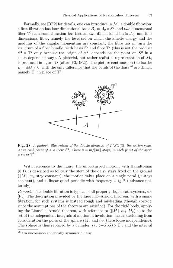
Physical Applications of Nekhoroshev Theorem 53
Formally, see [BF2] for details, one can introduce inM0 a double fibration:a first fibration has four dimensional basis B0 = A0×S2, and two dimensionalfiber T
2; a second fibration has instead two dimensional basis A0, and fourdimensional fiber, namely the level set on which the kinetic energy and themodulus of the angular momentum are constant; the fibre has in turn thestructure of a fiber bundle, with basis S2 and fibre T
2 (this is not the productS2 × T
2 only because the origin of g(i) depends on the point on S2 in achart dependent way). A pictorial, but rather realistic, representation ofM0
is produced in figure 28 (after [F2,BF2]). The picture continues on the borderL = ±G = 0, with the only difference that the petals of the daisy26 are thiner,namely T
1 in place of T2.
Fig. 28. A pictoric illustration of the double fibration of T ∗SO(3): the action spaceA; in each point of A a spere S2, where µ = m/‖m‖ stays; in each point of the sperea torus T
2.
With reference to the figure, the unperturbed motion, with Hamiltonian(6.1), is described as follows: the stem of the daisy stays fixed on the ground(‖M‖,m3 stay constant); the motion takes place on a single petal (µ staysconstant), and is linear quasi periodic with frequency ω (g(i), l advance uni-formly).Remark: The double fibration is typical of all properly degenerate systems, see[F3]. The description provided by the Liouville–Arnold theorem, with a singlefibration, for such systems is instead rough and misleading (though correct,since the assumptions of the theorem are satisfied). For the rigid body, apply-ing the Liouville–Arnold theorem, with reference to (‖M‖,m3,Mz) as to theset of the independent integrals of motion in involution, means excluding fromconsideration the poles of the sphere (Mz and m3 there loose independence).The sphere is thus replaced by a cylinder, say (−G,G)×T
1, and the interval
26 Un uncommon spherically symmetric daisy.
54 Giancarlo Benettin
(−G,G) is attached to A to form a three dimensional basis, while T1 is at-
tached to T2 to form T
3. This is a legitime but not sensible operation, whichintroduces spurious singularities in the foliation in correspondence of the ar-bitrarily chosen poles of the sphere. (By the way: dynamically, it is impossibleto stay consistently out of the poles, since nothing special is there.)
As a final comment on the unperturbed problem, it is worthwhile to noticethat h, as defined in (6.1), is always a quasi–convex function in A, though fornegative η it might appear similar to the counterexample (5.5). Indeed, anelementary computation shows that quasi–convexity of h is lost for (G,L) :L = ±G/√−η, but since η > − 1
2 , these points do not belong to A.
B. Results for Non Gyroscopic Motions
Now we enter the perturbed problem, namely the rigid body in a small po-sitional potential. Positional means that the potential depends only on theconfiguration R ∈ SO(3) of the body; correspondingly, the representative ofthe potential in each coordinate system is a homogeneous function of degreezero of the actions. From now on, it will be important to distinguish betweenfunctions defined intrinsically on the manifold, and their representatives inlocal coordinates. Local representatives will have an upper index (i), just aslocal coordinates; intrinsic functions will not. However, functions like the ki-netic energy h, which depend only on global coordinates, and therefore havethe same form in the different charts, with innocent abuse of the conven-tion will have no index, and will be confused with the corresponding functionM0 → R. So, we have an intrinsic Hamilton function H = h+ εf :M0 → R,which is represented locally by
H(i)(G,L, J (i), g(i), l, j(i))=h(G,L)+εf (i)(G,L, J (i), g(i), l, j(i)), i = 1, 2.(6.3)
It is worthwhile to remark that (due to the homogeneity property of f) thesystem has an elementary scaling property: indeed the change of variables
G = α G , L = α L , J (i) = α J (i)
(the angles being unchanged), canonically conjugates H(i) to
H(i)(G, L, J (i), g(i), l, j(i)) = h(G, L) + α−2εf (i)(G, L, J (i), g(i), l, j(i)) ;
this shows that it is equivalent to consider a rigid body in a small potential,that is a potential proportional to a small parameter ε, and a fast rigid bodywith initial actions Go, Lo, Jo multiplied by 1/
√ε, in an ε–independent po-
tential. In these lectures (at variance with [BF2,BFG1], and for homogeneitywith the other applications) we shall deal with initial actions of order one,and potential proportional to ε.
In each chart it is not difficult to work perturbatively, along the linesoutlined in Section 5, to eliminate “as far as possible” the dependence of the
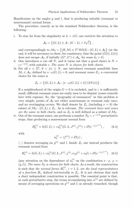
Physical Applications of Nekhoroshev Theorem 55
Hamiltonian on the angles g and l, that is producing suitable (resonant ornonresonant) normal forms.
The procedure, exactly as in the standard Nekhoroshev theorem, is thefollowing:
i. To stay far from the singularity at L = ±G, one restricts the attention to
Aδ =
(G,L) ∈ A : |G− L| > δ√ε
,
and correspondingly to Mδ =
(R,M) ∈ T ∗SO(3) : (G,L) ∈ Aδ
(at theend, it will be necessary to show, for consistency, that the point (G(t), L(t))does not escape Aδ, if initially (Go, Lo) ∈ Aδ0 for some δ0 > δ).
ii. One introduces a cut–off N , and it turns out that a good choice is N =c ε−1/4, with suitable c. The same N is chosen for both charts.
iii. For all ν ∈ Z2, 0 < |ν| ≤ N , one introduces resonant manifolds lines
Mν ∈ Aδ, defined by ν · ω(G,L) = 0, and resonant zones Zν ; a convenientchoice for the zones is
Zν =
(G,L) ∈ Aδ : |ν · ω(G,L)| < G/(2N |ν|)
.
If a neighborhood of the origin G = 0 is excluded, and is ε is sufficientlysmall, different resonant zones are easily seen to be disjoint (zones coincidehere with regions). So, the “geography of resonances” in this problem isvery simple: points of Aδ are either nonresonant or resonant only once,and no overlapping occurs. We shall denote by Zν (including ν = 0) thesubset of Mδ : (G,L) ∈ Zν . As is relevant, The resonant lines and zonesare the same in both charts, and so Zν is well defined as a subset ofMδ.
iv. Out of the resonant zones, one performs a numberN0 ∼ ε−1/4 perturbativesteps, thus producing a nonresonant normal form
H(i)0 = h(G,L) + εu
(i)0 (G,L, J (i), j(i)) +O(e−1/ε1/4
) , (6.4)
withu
(i)0 = 〈f (i)〉+O(ε) ;
〈 . 〉 denotes averaging on g(i) and l. Inside Zν one instead produces theresonant normal form
H(i)ν = h(G,L) + εu(i)
ν (G,L, J (i), j(i), ν1g(i) + ν2l) +O(e−1/ε1/4
) (6.5)
(pay attention on the dependence of u(i)ν on the combination ν · ϕ, ϕ =
(g, l)). The same N0 is chosen for both charts . As a result, the constructionis such that the normal forms H(i)
ν , i = 1, 2, are the local representativesof a function Hν defined intrinsically in Zν . It is not obvious that sucha chart independent construction is possible. The essential point is that,at each perturbative step, the terms accumulating into u(i) are defined bymeans of averaging operations on g(i) and l; as already remarked, though
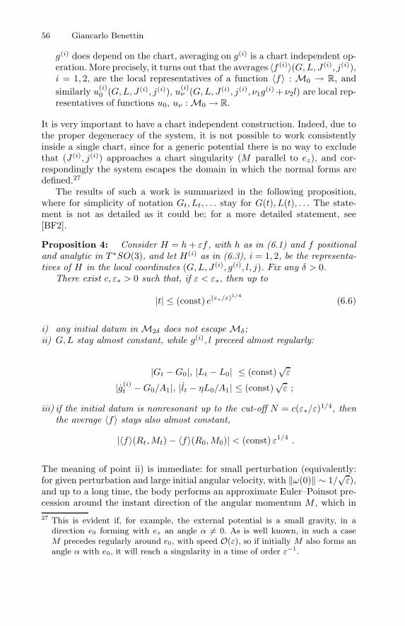
56 Giancarlo Benettin
g(i) does depend on the chart, averaging on g(i) is a chart independent op-eration. More precisely, it turns out that the averages 〈f (i)〉(G,L, J (i), j(i)),i = 1, 2, are the local representatives of a function 〈f〉 : M0 → R, andsimilarly u(i)
0 (G,L, J (i), j(i)), u(i)ν (G,L, J (i), j(i), ν1g
(i) + ν2l) are local rep-resentatives of functions u0, uν :M0 → R.
It is very important to have a chart independent construction. Indeed, due tothe proper degeneracy of the system, it is not possible to work consistentlyinside a single chart, since for a generic potential there is no way to excludethat (J (i), j(i)) approaches a chart singularity (M parallel to ez), and cor-respondingly the system escapes the domain in which the normal forms aredefined.27
The results of such a work is summarized in the following proposition,where for simplicity of notation Gt, Lt, . . . stay for G(t), L(t), . . . The state-ment is not as detailed as it could be; for a more detailed statement, see[BF2].
Proposition 4: Consider H = h+ εf , with h as in (6.1) and f positionaland analytic in T ∗SO(3), and let H(i) as in (6.3), i = 1, 2, be the representa-tives of H in the local coordinates (G,L, J (i), g(i), l, j). Fix any δ > 0.
There exist c, ε∗ > 0 such that, if ε < ε∗, then up to
|t| ≤ (const) e(ε∗/ε)1/4
(6.6)
i) any initial datum in M2δ does not escape Mδ;ii) G,L stay almost constant, while g(i), l preceed almost regularly:
|Gt −G0|, |Lt − L0| ≤ (const)√ε
|g(i)t −G0/A1|, |lt − ηL0/A1| ≤ (const)
√ε ;
iii) if the initial datum is nonresonant up to the cut-off N = c(ε∗/ε)1/4, thenthe average 〈f〉 stays also almost constant,
|〈f〉(Rt,Mt)− 〈f〉(R0,M0)| < (const) ε1/4 .
The meaning of point ii) is immediate: for small perturbation (equivalently:for given perturbation and large initial angular velocity, with ‖ω(0)‖ ∼ 1/
√ε),
and up to a long time, the body performs an approximate Euler–Poinsot pre-cession around the instant direction of the angular momentum M , which in27 This is evident if, for example, the external potential is a small gravity, in a
direction e0 forming with ez an angle α = 0. As is well known, in such a caseM precedes regularly around e0, with speed O(ε), so if initially M also forms anangle α with e0, it will reach a singularity in a time of order ε−1.
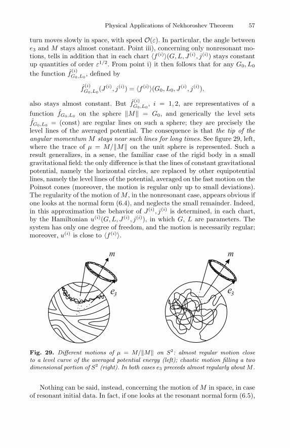
Physical Applications of Nekhoroshev Theorem 57
turn moves slowly in space, with speed O(ε). In particular, the angle betweene3 and M stays almost constant. Point iii), concerning only nonresonant mo-tions, tells in addition that in each chart 〈f (i)〉(G,L, J (i), j(i)) stays constantup quantities of order ε1/2. From point i) it then follows that for any G0, L0
the function f (i)G0,L0
, defined by
f(i)G0,L0
(J (i), j(i)) = 〈f (i)〉(G0, L0, J(i), j(i)),
also stays almost constant. But f (i)G0,L0
, i = 1, 2, are representatives of afunction fG0,L0 on the sphere ‖M‖ = G0, and generically the level setsfG0,L0 = (const) are regular lines on such a sphere; they are precisely thelevel lines of the averaged potential. The consequence is that the tip of theangular momentum M stays near such lines for long times. See figure 29, left,where the trace of µ = M/‖M‖ on the unit sphere is represented. Such aresult generalizes, in a sense, the familiar case of the rigid body in a smallgravitational field: the only difference is that the lines of constant gravitationalpotential, namely the horizontal circles, are replaced by other equipotentiallines, namely the level lines of the potential, averaged on the fast motion on thePoinsot cones (moreover, the motion is regular only up to small deviations).The regularity of the motion ofM , in the nonresonant case, appears obvious ifone looks at the normal form (6.4), and neglects the small remainder. Indeed,in this approximation the behavior of J (i), j(i) is determined, in each chart,by the Hamiltonian u(i)(G,L, J (i), j(i)), in which G, L are parameters. Thesystem has only one degree of freedom, and the motion is necessarily regular;moreover, u(i) is close to 〈f (i)〉.
Fig. 29. Different motions of µ = M/‖M‖ on S2: almost regular motion closeto a level curve of the averaged potential energy (left); chaotic motion filling a twodimensional portion of S2 (right). In both cases e3 preceeds almost regularly about M .
Nothing can be said, instead, concerning the motion of M in space, in caseof resonant initial data. In fact, if one looks at the resonant normal form (6.5),
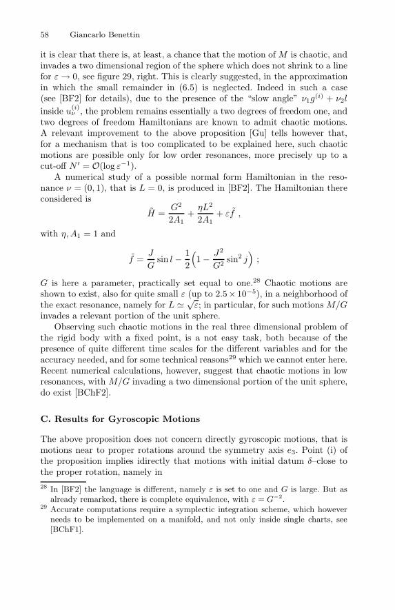
58 Giancarlo Benettin
it is clear that there is, at least, a chance that the motion of M is chaotic, andinvades a two dimensional region of the sphere which does not shrink to a linefor ε→ 0, see figure 29, right. This is clearly suggested, in the approximationin which the small remainder in (6.5) is neglected. Indeed in such a case(see [BF2] for details), due to the presence of the “slow angle” ν1g
(i) + ν2l
inside u(i)ν , the problem remains essentially a two degrees of freedom one, and
two degrees of freedom Hamiltonians are known to admit chaotic motions.A relevant improvement to the above proposition [Gu] tells however that,for a mechanism that is too complicated to be explained here, such chaoticmotions are possible only for low order resonances, more precisely up to acut-off N ′ = O(log ε−1).
A numerical study of a possible normal form Hamiltonian in the reso-nance ν = (0, 1), that is L = 0, is produced in [BF2]. The Hamiltonian thereconsidered is
H =G2
2A1+ηL2
2A1+ εf ,
with η,A1 = 1 and
f =J
Gsin l − 1
2
(
1− J2
G2sin2 j
)
;
G is here a parameter, practically set equal to one.28 Chaotic motions areshown to exist, also for quite small ε (up to 2.5× 10⁻⁵), in a neighborhood ofthe exact resonance, namely for L
√ε; in particular, for such motions M/G
invades a relevant portion of the unit sphere.Observing such chaotic motions in the real three dimensional problem of
the rigid body with a fixed point, is a not easy task, both because of thepresence of quite different time scales for the different variables and for theaccuracy needed, and for some technical reasons29 which we cannot enter here.Recent numerical calculations, however, suggest that chaotic motions in lowresonances, with M/G invading a two dimensional portion of the unit sphere,do exist [BChF2].
C. Results for Gyroscopic Motions
The above proposition does not concern directly gyroscopic motions, that ismotions near to proper rotations around the symmetry axis e3. Point (i) ofthe proposition implies idirectly that motions with initial datum δ–close tothe proper rotation, namely in28 In [BF2] the language is different, namely ε is set to one and G is large. But as
already remarked, there is complete equivalence, with ε = G−2.29 Accurate computations require a symplectic integration scheme, which however
needs to be implemented on a manifold, and not only inside single charts, see[BChF1].
Physical Applications of Nekhoroshev Theorem 59
Mδ =M\Mδ ,
cannot escapeM2δ for the long time scale (6.6). That is: gyroscopic motionsremain gyroscopic for long time. But this is a poor result, since it does nottell anything on the motion of the angular momentum M in space, though itstates that e3 in any case closely follows M .
To understand the behavior of M , and prove the equivalent of points (ii)and (iii) for gyroscopic motions, one must learn to work perturbatively aroundsingularities of the action–angle variables, or in geometric words, around sin-gularities of the foliation of the phase space into invariant tori. As alreadyremarked, this is a rather general problem in perturbation theory. We arehere confronted with it in connection with the gyroscopic motions of the rigidbody, but we shall be confronted with it in the next sections too, dealing withthe problem of the stability of the Lagrangian equilibrium points L4, L5 inthe circular restricted three body problem.
For the rigid body, the perturbative construction goes through the follow-ing steps:
i. One introduces new canonical action - angle variables(Γ,Λ, γ(i), λ) “adapted to the singlularity”, namely
Γ = G , Λ = G− L , γ(i) = g(i) + l , λ = −l ,
(J (i), j(i)) remaining unchanged. The singularity L = G (for symmetry,we can restrict the attention only to it) corresponds now to Λ = 0, andone easily sees that only the pair (Λ, λ) is there singular, while (Γ, γ(i))is regular; in particular (look at figure 27), the angle γ(i) becomes equal,on the singularity, to the angle of proper rotation, usually called ψ, ofthe familiar Euler coordinates (in the same limit, j(i) gets equal to theprecession ϕ of e3 about ez).
ii. The polar–like coordinates Λ, λ are replaced by Cartesian–like coordinatesx, y, via
x =√
2Λ cosλ , y =√
2Λ sinλ ,
and it turns out [NL] (see also [BFG1]) that (Γ, γ(i), x, y, J (i), j(i)), i = 1, 2,provide an analytic atlas in the “North emisphere”
M+ =
(R,M) ∈ T ∗SO(3) : m3 > 0
(the chart singularity moved to the equator). It turns out that
x =√
2m2√Γ − Λ
, y =√
2m1√Γ − Λ
.
The Hamiltonian, in each chart, gets the form
K(i)(Γ, γ(i), x, y, J (i), j(i)) = k(Γ,Λ(x, y)) + εΦ(i)(Γ, γ(i), x, y, J (i), j(i)) ,
60 Giancarlo Benettin
with Λ(x, y) = 12 (x2 + y2) and
k(Γ,Λ) =1
2A3[Γ 2 + βΛ2 − 2βΓΛ] ,
withβ = 1− A3
A1, −1 < β < 1 . (6.7)
The domain of K(i) is such that
G > 0 , 0 ≤ Λ(x, y) < G , |J (i)| < G , g(i), j(i) ∈ T2 .
It should be stressed that Λ here is not a coordinate, but a (nonsingular)function of x and y. A further change of coordinates, widely used afterBirkhoff in connection with perturbation theory in Cartesian coordinates,turns out to be useful, namely the passage to the complex canonical coor-dinates
w =y − ixi√
2, z =
y + ix√2
;
out of the singularity it is
w =√Λe−iλ , z =
√Λeiλ , Λ = −iwz .
With little abuse of notation, though we changed variables from x, y tow, z, we do not change the names of functions.
iii. Resonant and nonresonant normal forms are constructed. The constructionof normal forms in Cartesian coordinates is a well established procedurein the isochronous case (in our notations, for k linear in Λ). In the nonisochronous case, however, some care must be paid, due to the presenceof non constant small denominators, which alter in an essential way theBirkhoff construction. The procedure to be followed, see [SM] and [BGF], isconceptually simple: in the very essence, the idea is to use coordinates w, z,but to proceed perturbatively — with Fourier developments, ultravioletcut-off and so on — as if Λ, λ were coordinates.
To this purpose, one first introduces the frequency
ω(Γ,Λ) =1A3
(Γ − βΛ,−β(Γ − Λ)) ,
which is well defined on the singularity, too, where
ω → ω0 =Γ
A3(1,−β) .
As is remarkable, gyroscopic motions are resonant or nonresonant (for agiven cut-off) depending only on β, that is on the geometry of the body,and on ε. The two components of ω0 are easily interpreted as the frequency
Physical Applications of Nekhoroshev Theorem 61
of the rotation about e3, and of the small oscillations of e3 around M inthe Euler–Poinsot motion. For the perturbation, as well as for any analyticfunction F :M→ R, F (i)(Γ, g(i), w, z, J (i), j(i)), one defines the “Fourierseries”,
F (i) =∑
ν∈Z2
F (i)ν (Γ,Λ, J (i), j(i))E(i)
ν (g(i), w, z) ,
(Λ stays now for the product iwz), with F (i) analytic, and
E(i)ν =
eiν1γ(i)wν2 for ν2 < 0
eiν1γ(i)zν2 for ν2 ≥ 0.
As is quite important, the above development in Fourier series is intrin-sic: namely, although F (i)
ν and E(i)ν are only local, the product F (i)
ν E(i)ν is
nevertheless the representative of an intrinsic “Fourier component”, anda Fourier series is well defined on the manifold (see [BFG1] for details).Once the Fourier series is defined, it is sensible to introduce the ultravi-olet cut-off N , and the resonant and nonresonant zones, as in the caseof nonresonant motions. However, having in mind to work only in a smallneighborhoodMδ of the proper rotation, of size ε1/2, it is enough to intro-duce just a single zone, either resonant or nonresonant depending on ω0,and work consistently inside it. So, for gyroscopic motions, being resonantor nonresonant does not depend on the initial datum, but on β, that is onthe geometry of the body.The nonresonant normal form, for example, looks in each chart
K(i)0 = k(Γ,Λ(x, y)) + εu
(i)0 (Γ,Λ(x, y), J (i), j(i)) +O(e−1/ε1/4
) ,
with u(i)0 close to the average 〈Φ(i)〉; all of these functions are local repre-
sentatives of functions on the manifold.
As a matter of fact, following this road one proves a proposition that, essen-tially, extend to the gyroscopic motions the results of Proposition 4.
Proposition 5: Let H = h+ εf be as in Proposition 4, with f analytic ina neighborhood of the proper rotations, too. There exist δ, c, ε∗ > 0 such that,if ε < ε∗, then up to
|t| ≤ (const) e(ε∗/ε)1/4
(6.8)
i) any initial datum in Mδ does not escape M2δ;ii) Γ,Λ stay almost constant, and γ(i) advances almost regularly:
|Γt − Γ0|, |Λt − Λ0| ≤ (const)√ε , |γ(i)
t − βΓ0/A3| ≤ (const)√ε ;
iii) if β is nonresonant up to the cut-off N = c(ε∗/ε)1/4, then the average 〈f〉stays also almost constant,
|〈f〉(Rt,Mt)− 〈f〉(R0,M0)| < (const) ε1/4 .
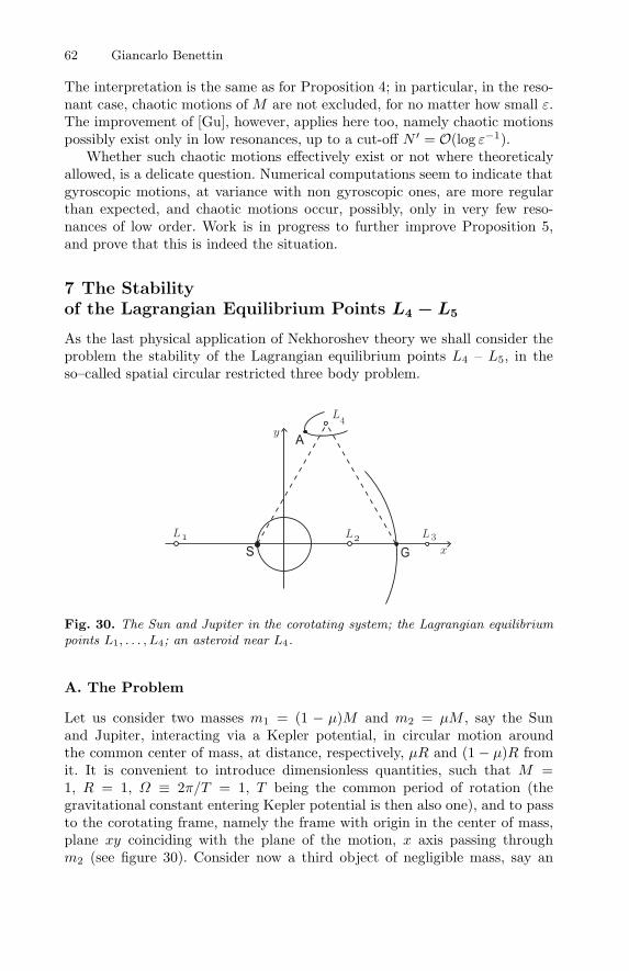
62 Giancarlo Benettin
The interpretation is the same as for Proposition 4; in particular, in the reso-nant case, chaotic motions of M are not excluded, for no matter how small ε.The improvement of [Gu], however, applies here too, namely chaotic motionspossibly exist only in low resonances, up to a cut-off N ′ = O(log ε−1).
Whether such chaotic motions effectively exist or not where theoreticalyallowed, is a delicate question. Numerical computations seem to indicate thatgyroscopic motions, at variance with non gyroscopic ones, are more regularthan expected, and chaotic motions occur, possibly, only in very few reso-nances of low order. Work is in progress to further improve Proposition 5,and prove that this is indeed the situation.
7 The Stabilityof the Lagrangian Equilibrium Points L4 − L5
As the last physical application of Nekhoroshev theory we shall consider theproblem the stability of the Lagrangian equilibrium points L4 – L5, in theso–called spatial circular restricted three body problem.
Fig. 30. The Sun and Jupiter in the corotating system; the Lagrangian equilibriumpoints L1, . . . , L4; an asteroid near L4.
A. The Problem
Let us consider two masses m1 = (1 − µ)M and m2 = µM , say the Sunand Jupiter, interacting via a Kepler potential, in circular motion aroundthe common center of mass, at distance, respectively, µR and (1 − µ)R fromit. It is convenient to introduce dimensionless quantities, such that M =1, R = 1, Ω ≡ 2π/T = 1, T being the common period of rotation (thegravitational constant entering Kepler potential is then also one), and to passto the corotating frame, namely the frame with origin in the center of mass,plane xy coinciding with the plane of the motion, x axis passing throughm2 (see figure 30). Consider now a third object of negligible mass, say an
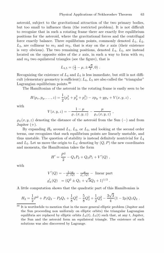
Physical Applications of Nekhoroshev Theorem 63
asteroid, subject to the gravitational attraction of the two primary bodies,but too small to influence them (the restricted problem). It is not difficultto recognize that in such a rotating frame there are exactly five equilibriumpositions for the asteroid, where the gravitational forces and the centrifugalforce exactly balance. Three equilibrium points, commonly denoted L1, L2,L3, are collinear to m1 and m2, that is stay on the x axis (their existenceis very obvious). The two remaining positions, denoted L4, L5, are insteadlocated on the opposite sides of the x axis, in such a way to form with m1
and m2 two equilateral triangles (see the figure), that is
L4,5 = (12 − µ,±
√3
2 , 0) .
Recognizing the existence of L4 and L5 is less immediate, but still is not diffi-cult (elementary geometry is sufficient); L4, L5 are also called the “triangular”Lagrangian equilibrium points.30
The Hamiltonian of the asteroid in the rotating frame is easily seen to be
H(px, py, . . . , z) =12(p2x + p2
y + p2z)− xpy + ypx + V (x, y, z) ,
withV (x, y, z) = − 1− µ
−(x, y, z)− µ
+(x, y, z),
±(x, y, z) denoting the distance of the asteroid from the Sun (−) and fromJupiter (+).
By expanding H0 around L1, L2, or L3, and looking at the second orderterms, one recognizes that such equilibrium points are linearly unstable, andthus unstable. The question of stability is instead definitely nontrivial for L4
and L5. Let us move the origin to L4; denoting by (Q,P ) the new coordinatesand momenta, the Hamiltonian takes the form
H ′ =P 2
2−Q1P2 +Q2P1 + V ′(Q) ,
with
V ′(Q) = − 1−µ′−(Q) −
µ′+(Q) − linear part
′±(Q) = (Q2 ±Q1 +√
3Q2 + 1)1/2 .
A little computation shows that the quadratic part of this Hamiltonian is
H2 =12P 2 + P1Q2 − P2Q1 +
18Q2
1 −58Q2
2 +12Q2
3 −3√
34
(1− 2µ)Q1Q2 .
30 It is worthwhile to mention that in the more general elliptic problem (Jupiter andthe Sun proceeding non uniformly on elliptic orbits) the triangular Lagrangianequilibria are replaced by elliptic orbits L4(t), L5(t) such that, at any t, Jupiter,the Sun and the asteroid form an equilateral triangle. The existence of suchsolutions was also discovered by Lagrange.
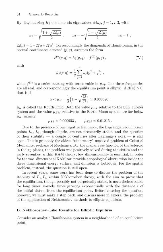
64 Giancarlo Benettin
By diagonalizing H2 one finds six eigenvalues ±iωj, j = 1, 2, 3, with
ω1 =
√
1 +√
∆(µ)2
, ω2 = −
√
1−√
∆(µ)2
, ω3 = 1 ,
∆(µ) = 1−27µ+27µ2. Correspondingly the diagonalized Hamiltonian, in thenormal coordinates denoted (p, q), assumes the form
H ′′(p, q) = h2(p, q) + f (3)(p, q) , (7.1)
with
h2(p, q) =12
3∑
j=1
ωj(p2j + q2j ) ,
while f (3) is a series starting with terms cubic in p, q. The three frequenciesare all real, and correspondingly the equilibrium point is elliptic, if ∆(µ) > 0,that is if
µ < µR =12
(
1−√
2327
)
0.038520 ;
µR is called the Routh limit. Both the value µSJ relative to the Sun–Jupitersystem and the value µEM relative to the Earth–Moon system are far belowµR, namely
µSJ 0.000953 , µEM 0.01215 .
Due to the presence of one negative frequency, the Lagrangian equilibriumpoints L4, L5, though elliptic, are not necessarily stable, and the questionof their stability — a couple of centuries after Lagrange’s work — is stillopen. This is probably the oldest “elementary” unsolved problem of CelestialMechanics, perhaps of Mechanics. For the planar case (motion of the asteroidin the xy plane), the problem was positively solved during the sixties and theearly seventies, within KAM theory; low dimensionality is essential, in orderfor the two–dimensional KAM tori provide a topological obstruction inside thethree dimensional energy surface, and diffusion is forbidden. For the spatialproblem, instead, the question is still open.
In recent years, some work has been done to discuss the problem of thestability of L4, L5 within Nekhoroshev theory, with the aim to prove thatthe equilibrium, though possibly not perpetually stable, is nevertheless stablefor long times, namely times growing exponentially with the distance ε ofthe initial datum from the equilibrium point. Before entering the question,however, we must make a step back, and discuss more in general the problemof the application of Nekhoroshev methods to elliptic equilibria.
B. Nekhoroshev–Like Results for Elliptic Equiliria
Consider an analytic Hamiltonian system in a neighborhood of an equilibriumpoint,
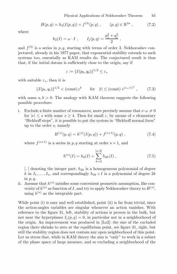
Physical Applications of Nekhoroshev Theorem 65
H(p, q) = h2(I(p, q)) + f (3)(p, q) , (p, q) ∈ R2n , (7.2)
where
h2(I) = ω · I , Ij(p, q) =p2j + q2j
2,
and f (3) is a series in p, q, starting with terms of order 3. Nekhoroshev con-jectured, already in his 1977 paper, that exponential stability extends to suchsystems too, essentially as KAM results do. The conjectured result is thusthat, if the initial datum is sufficiently close to the origin, say if
ε := ‖I(p0, q0)‖1/2 ≤ ε∗
with suitable ε∗, then it is
‖I(pt, qt)‖1/2 < (const) εb for |t| ≤ (const) e(ε∗/ε)a
, (7.3)
with some a, b > 0. The analogy with KAM theorem suggests the followingpossible procedure:
i. Exclude a finite number of resonances, more precisely assume that ν ·ω = 0for |ν| ≤ s with some s ≥ 4. Then for small ε, by means of s elementary“Birkhoff steps”, it is possible to put the system in “Birkhoff normal form”up to the order s, namely
H(s)(p, q) = h(s)(I(p, q)) + f (s+1)(p, q) , (7.4)
where f (s+1) is a series in p, q starting at order s+ 1, and
h(s)(I) = h2(I) +[s/2]∑
k=2
h2k(I) , (7.5)
[ . ] denoting the integer part; h2k is a homogeneous polynomial of degreek in I1, . . . , In, and correspondingly h2k I is a polynomial of degree 2kin p, q.
ii. Assume that h(s) satisfies some convenient geometric assumption, like con-vexity of h(s) as function of I, and try to apply Nekhoroshev theory toH(s),using h(s) as the integrable part.
While point (i) is easy and well established, point (ii) is far from trivial, sincethe action-angles variables are singular whenever an action vanishes. Withreference to the figure 31, left, stability of actions is proven in the bulk, butnot near the hyperplanes Ij(p, q) = 0, in particular not in a neighborhood ofthe origin. An improvement was produced in [Lo2]: the size of the excludedregion there shrinks to zero at the equilibrium point, see figure 31, right, butstill the stability region does not contain any open neighborhood of this point.Let us stress that, while in KAM theory the aim is “only” to work in a subsetof the phase space of large measure, and so excluding a neighborhood of the
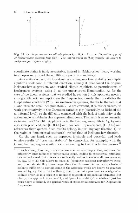
66 Giancarlo Benettin
Fig. 31. In a layer around coordinate planes Ij = 0, j = 1, . . . , n, the ordinary proofof Nekhoroshev theorem fails (left). The improvement in [Lo2] reduces the layers towedge–shaped regions (right).
coordinate plains is fairly acceptable, instead in Nekhoroshev theory workingin an open set around the equilibrium point is mandatory.
As a matter of fact, the literature concerning long time stability for ellipticequilibria took soon a different direction, namely it abandoned the originalNekhoroshev suggestion, and studied elliptic equilibria as perturbations ofisochronous systems, using h2 as the unperturbed Hamiltonian. As for thecase of the linear systems that we studied in Section 2, this approach needs astrong arithmetic assumption on the frequencies, namely that ω satisfies theDiophantine condition (2.3). For isochronous systems, thanks to the fact thatω and thus the small denominators ν · ω are constant, it is rather natural towork perturbatively in the Cartesian variables p, q (essentially as Birkhoff didat a formal level), so the difficulty connected with the lack of analyticity of theaction angle variables in this approach disappears. The result is an exponentialestimate like (7.3) [Gi1]. Applications to the Lagrangian equilibria L4, L5 werealso soon produced; see [GDFGS] and, for later improvements, [GS,Gi2] andreferences there quoted. Such results belong, in our language (Section 1), tothe realm of “exponential estimates”, rather than of Nekhoroshev theorem.
On the one hand, such an approach is simple and powerful, and leadsto nice results of “practical stability” in connection, for example, with thetriangular Lagrangian equilibria corresponding to the Sun-Jupiter masses.31
31 In such a case, of course, it is not known whether ω is Diophantine, and thus if anarbitrarily large number of perturbative steps, leading to exponential estimates,can be performed. But ω is known sufficiently well as to exclude all resonances upto, say, |ν| = 30; this allows to make 30 (computer assisted) perturbative steps,and to obtain stability times larger than the Universe lifetime, with a basin ofstability sufficient to contain some of the asteroids which are known to gravitatearound L4, L5. Perturbation theory, due to the finite precision knowledge of ω,is finite order, so in a sense it is improper to speak of exponential estimates. Butclearly, the approach is successful, and “practical stability” is acheived, just be-cause there is, behind, the general result of exponential estimates for Diophantinefrequencies.
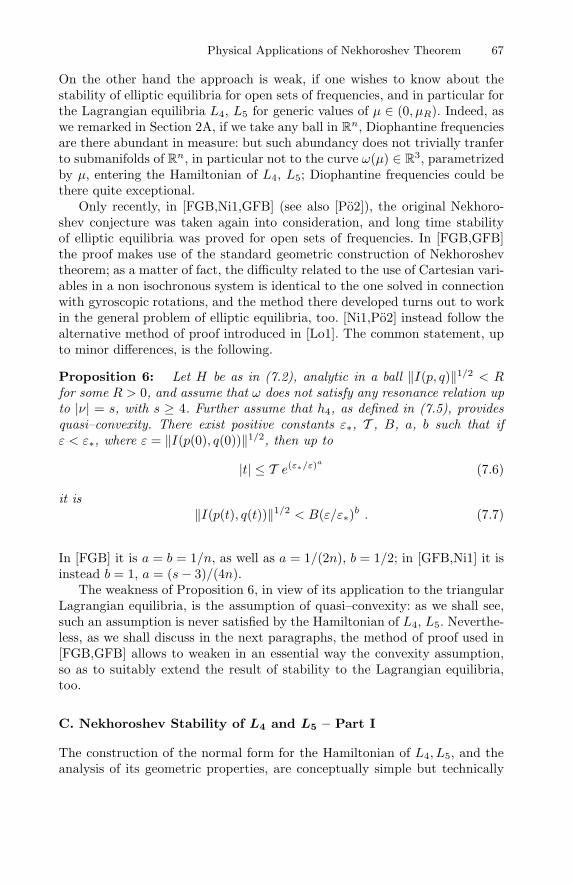
Physical Applications of Nekhoroshev Theorem 67
On the other hand the approach is weak, if one wishes to know about thestability of elliptic equilibria for open sets of frequencies, and in particular forthe Lagrangian equilibria L4, L5 for generic values of µ ∈ (0, µR). Indeed, aswe remarked in Section 2A, if we take any ball in R
n, Diophantine frequenciesare there abundant in measure: but such abundancy does not trivially tranferto submanifolds of R
n, in particular not to the curve ω(µ) ∈ R3, parametrized
by µ, entering the Hamiltonian of L4, L5; Diophantine frequencies could bethere quite exceptional.
Only recently, in [FGB,Ni1,GFB] (see also [Po2]), the original Nekhoro-shev conjecture was taken again into consideration, and long time stabilityof elliptic equilibria was proved for open sets of frequencies. In [FGB,GFB]the proof makes use of the standard geometric construction of Nekhoroshevtheorem; as a matter of fact, the difficulty related to the use of Cartesian vari-ables in a non isochronous system is identical to the one solved in connectionwith gyroscopic rotations, and the method there developed turns out to workin the general problem of elliptic equilibria, too. [Ni1,Po2] instead follow thealternative method of proof introduced in [Lo1]. The common statement, upto minor differences, is the following.
Proposition 6: Let H be as in (7.2), analytic in a ball ‖I(p, q)‖1/2 < Rfor some R > 0, and assume that ω does not satisfy any resonance relation upto |ν| = s, with s ≥ 4. Further assume that h4, as defined in (7.5), providesquasi–convexity. There exist positive constants ε∗, T , B, a, b such that ifε < ε∗, where ε = ‖I(p(0), q(0))‖1/2, then up to
|t| ≤ T e(ε∗/ε)a
(7.6)
it is‖I(p(t), q(t))‖1/2 < B(ε/ε∗)b . (7.7)
In [FGB] it is a = b = 1/n, as well as a = 1/(2n), b = 1/2; in [GFB,Ni1] it isinstead b = 1, a = (s− 3)/(4n).
The weakness of Proposition 6, in view of its application to the triangularLagrangian equilibria, is the assumption of quasi–convexity: as we shall see,such an assumption is never satisfied by the Hamiltonian of L4, L5. Neverthe-less, as we shall discuss in the next paragraphs, the method of proof used in[FGB,GFB] allows to weaken in an essential way the convexity assumption,so as to suitably extend the result of stability to the Lagrangian equilibria,too.
C. Nekhoroshev Stability of L4 and L5 – Part I
The construction of the normal form for the Hamiltonian of L4, L5, and theanalysis of its geometric properties, are conceptually simple but technically
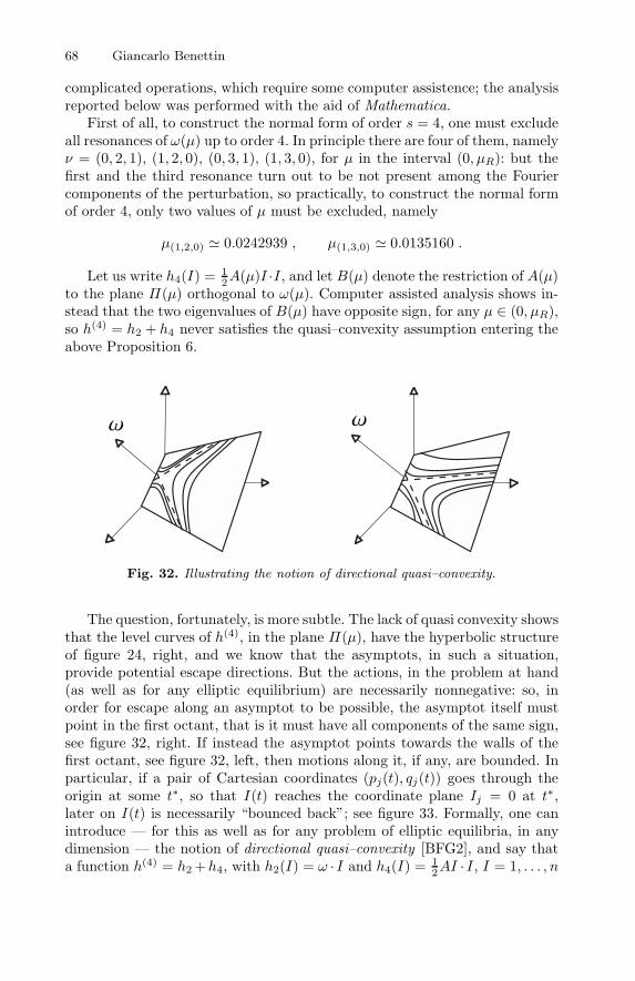
68 Giancarlo Benettin
complicated operations, which require some computer assistence; the analysisreported below was performed with the aid of Mathematica.
First of all, to construct the normal form of order s = 4, one must excludeall resonances of ω(µ) up to order 4. In principle there are four of them, namelyν = (0, 2, 1), (1, 2, 0), (0, 3, 1), (1, 3, 0), for µ in the interval (0, µR): but thefirst and the third resonance turn out to be not present among the Fouriercomponents of the perturbation, so practically, to construct the normal formof order 4, only two values of µ must be excluded, namely
µ(1,2,0) 0.0242939 , µ(1,3,0) 0.0135160 .
Let us write h4(I) = 12A(µ)I ·I, and let B(µ) denote the restriction of A(µ)
to the plane Π(µ) orthogonal to ω(µ). Computer assisted analysis shows in-stead that the two eigenvalues of B(µ) have opposite sign, for any µ ∈ (0, µR),so h(4) = h2 + h4 never satisfies the quasi–convexity assumption entering theabove Proposition 6.
Fig. 32. Illustrating the notion of directional quasi–convexity.
The question, fortunately, is more subtle. The lack of quasi convexity showsthat the level curves of h(4), in the plane Π(µ), have the hyperbolic structureof figure 24, right, and we know that the asymptots, in such a situation,provide potential escape directions. But the actions, in the problem at hand(as well as for any elliptic equilibrium) are necessarily nonnegative: so, inorder for escape along an asymptot to be possible, the asymptot itself mustpoint in the first octant, that is it must have all components of the same sign,see figure 32, right. If instead the asymptot points towards the walls of thefirst octant, see figure 32, left, then motions along it, if any, are bounded. Inparticular, if a pair of Cartesian coordinates (pj(t), qj(t)) goes through theorigin at some t∗, so that I(t) reaches the coordinate plane Ij = 0 at t∗,later on I(t) is necessarily “bounced back”; see figure 33. Formally, one canintroduce — for this as well as for any problem of elliptic equilibria, in anydimension — the notion of directional quasi–convexity [BFG2], and say thata function h(4) = h2 +h4, with h2(I) = ω · I and h4(I) = 1
2AI · I, I = 1, . . . , n
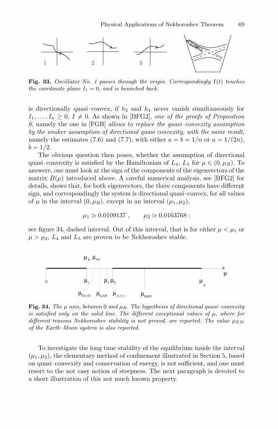
Physical Applications of Nekhoroshev Theorem 69
Fig. 33. Oscillator No. 1 passes through the origin. Correspondingly I(t) touchesthe coordinate plane I1 = 0, and is bounched back.
is directionally quasi–convex, if h2 and h4 never vanish simultaneously forI1, . . . , In ≥ 0, I = 0. As shown in [BFG2], one of the proofs of Proposition6, namely the one in [FGB] allows to replace the quasi–convexity assumptionby the weaker assumption of directional quasi convexity, with the same result,namely the estimates (7.6) and (7.7), with either a = b = 1/n or a = 1/(2n),b = 1/2.
The obvious question then poses, whether the assumption of directionalquasi–convexity is satisfied by the Hamiltonian of L4, L5 for µ ∈ (0, µR). Toanswere, one must look at the sign of the components of the eigenvectors of thematrix B(µ) introduced above. A careful numerical analysis, see [BFG2] fordetails, shows that, for both eigenvectors, the three components have differentsign, and correspondingly the system is directional quasi–convex, for all valuesof µ in the interval (0, µR), except in an interval (µ1, µ2),
µ1 0.0109137 , µ2 0.0163768 ;
see figure 34, dashed interval. Out of this interval, that is for either µ < µ1 orµ > µ2, L4 and L5 are proven to be Nekhoroshev stable.
EM
0
4
(0,3,1)
Fig. 34. The µ axis, between 0 and µR. The hypothesis of directional quasi–convexityis satisfied only on the solid line. The different exceptional values of µ, where fordifferent reasons Nekhoroshev stability is not proved, are reported. The value µEM
of the Earth–Moon system is also reported.
To investigate the long time stability of the equilibrium inside the interval(µ1, µ2), the elementary method of confinement illustrated in Section 5, basedon quasi–convexity and conservation of energy, is not sufficient, and one mustresort to the not easy notion of steepness. The next paragraph is devoted toa short illustration of this not much known property.
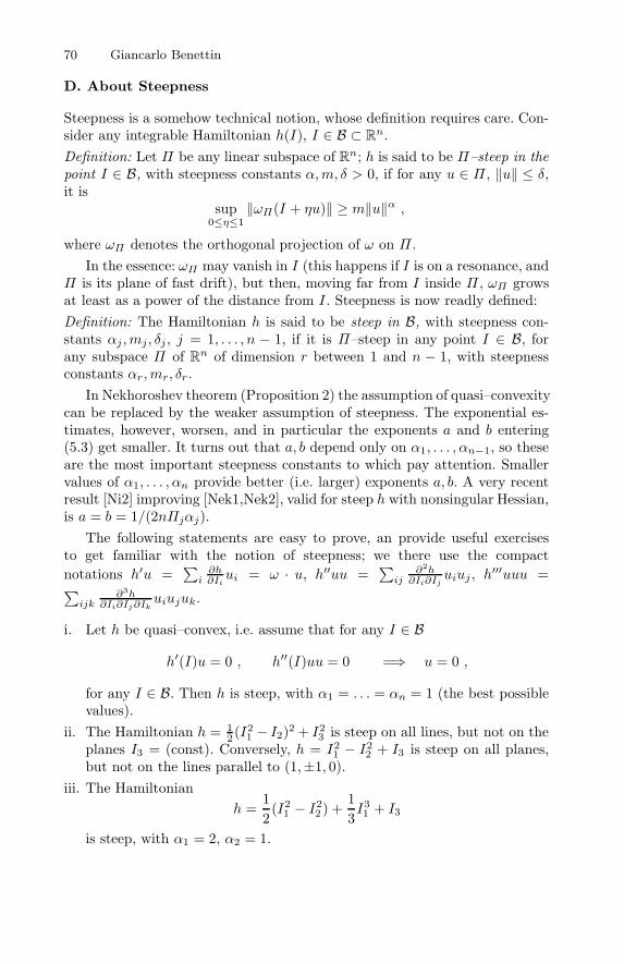
70 Giancarlo Benettin
D. About Steepness
Steepness is a somehow technical notion, whose definition requires care. Con-sider any integrable Hamiltonian h(I), I ∈ B ⊂ R
n.Definition: Let Π be any linear subspace of R
n; h is said to be Π–steep in thepoint I ∈ B, with steepness constants α,m, δ > 0, if for any u ∈ Π , ‖u‖ ≤ δ,it is
sup0≤η≤1
‖ωΠ(I + ηu)‖ ≥ m‖u‖α ,
where ωΠ denotes the orthogonal projection of ω on Π .In the essence: ωΠ may vanish in I (this happens if I is on a resonance, and
Π is its plane of fast drift), but then, moving far from I inside Π , ωΠ growsat least as a power of the distance from I. Steepness is now readly defined:Definition: The Hamiltonian h is said to be steep in B, with steepness con-stants αj ,mj, δj , j = 1, . . . , n − 1, if it is Π–steep in any point I ∈ B, forany subspace Π of R
n of dimension r between 1 and n − 1, with steepnessconstants αr,mr, δr.
In Nekhoroshev theorem (Proposition 2) the assumption of quasi–convexitycan be replaced by the weaker assumption of steepness. The exponential es-timates, however, worsen, and in particular the exponents a and b entering(5.3) get smaller. It turns out that a, b depend only on α1, . . . , αn−1, so theseare the most important steepness constants to which pay attention. Smallervalues of α1, . . . , αn provide better (i.e. larger) exponents a, b. A very recentresult [Ni2] improving [Nek1,Nek2], valid for steep h with nonsingular Hessian,is a = b = 1/(2nΠjαj).
The following statements are easy to prove, an provide useful exercisesto get familiar with the notion of steepness; we there use the compactnotations h′u =
∑
i∂h∂Iiui = ω · u, h′′uu =
∑
ij∂2h∂Ii∂Ij
uiuj , h′′′uuu =∑
ijk∂3h
∂Ii∂Ij∂Ikuiujuk.
i. Let h be quasi–convex, i.e. assume that for any I ∈ B
h′(I)u = 0 , h′′(I)uu = 0 =⇒ u = 0 ,
for any I ∈ B. Then h is steep, with α1 = . . . = αn = 1 (the best possiblevalues).
ii. The Hamiltonian h = 12 (I2
1 − I2)2 + I23 is steep on all lines, but not on the
planes I3 = (const). Conversely, h = I21 − I2
2 + I3 is steep on all planes,but not on the lines parallel to (1,±1, 0).
iii. The Hamiltonianh =
12(I2
1 − I22 ) +
13I31 + I3
is steep, with α1 = 2, α2 = 1.
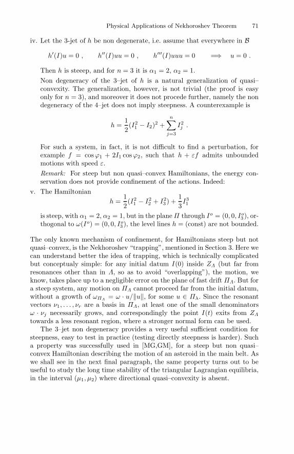
Physical Applications of Nekhoroshev Theorem 71
iv. Let the 3-jet of h be non degenerate, i.e. assume that everywhere in B
h′(I)u = 0 , h′′(I)uu = 0 , h′′′(I)uuu = 0 =⇒ u = 0 .
Then h is steeep, and for n = 3 it is α1 = 2, α2 = 1.Non degeneracy of the 3–jet of h is a natural generalization of quasi–convexity. The generalization, however, is not trivial (the proof is easyonly for n = 3), and moreover it does not procede further, namely the nondegeneracy of the 4–jet does not imply steepness. A counterexample is
h =12(I2
1 − I2)2 +n∑
j=3
I2j .
For such a system, in fact, it is not difficult to find a perturbation, forexample f = cosϕ1 + 2I1 cosϕ2, such that h + εf admits unboundedmotions with speed ε.Remark: For steep but non quasi–convex Hamiltonians, the energy con-servation does not provide confinement of the actions. Indeed:
v. The Hamiltonianh =
12(I2
1 − I22 + I2
3 ) +13I31
is steep, with α1 = 2, α2 = 1, but in the planeΠ through Io = (0, 0, Io3 ), or-thogonal to ω(Io) = (0, 0, Io3 ), the level lines h = (const) are not bounded.
The only known mechanism of confinement, for Hamiltonians steep but notquasi–convex, is the Nekhoroshev “trapping”, mentioned in Section 3. Here wecan understand better the idea of trapping, which is technically complicatedbut conceptualy simple: for any initial datum I(0) inside ZΛ (but far fromresonances other than in Λ, so as to avoid “overlapping”), the motion, weknow, takes place up to a negligible error on the plane of fast drift ΠΛ. But fora steep system, any motion on ΠΛ cannot proceed far from the initial datum,without a growth of ωΠΛ = ω · u/‖u‖, for some u ∈ Πλ. Since the resonantvectors ν1, . . . , νr are a basis in ΠΛ, at least one of the small denominatorsω · νj necessarily grows, and correspondingly the point I(t) exits from ZΛtowards a less resonant region, where a stronger normal form can be used.
The 3–jet non degeneracy provides a very useful sufficient condition forsteepness, easy to test in practice (testing directly steepness is harder). Sucha property was successfully used in [MG,GM], for a steep but non quasi–convex Hamiltonian describing the motion of an asteroid in the main belt. Aswe shall see in the next final paragraph, the same property turns out to beuseful to study the long time stability of the triangular Lagrangian equilibria,in the interval (µ1, µ2) where directional quasi–convexity is absent.
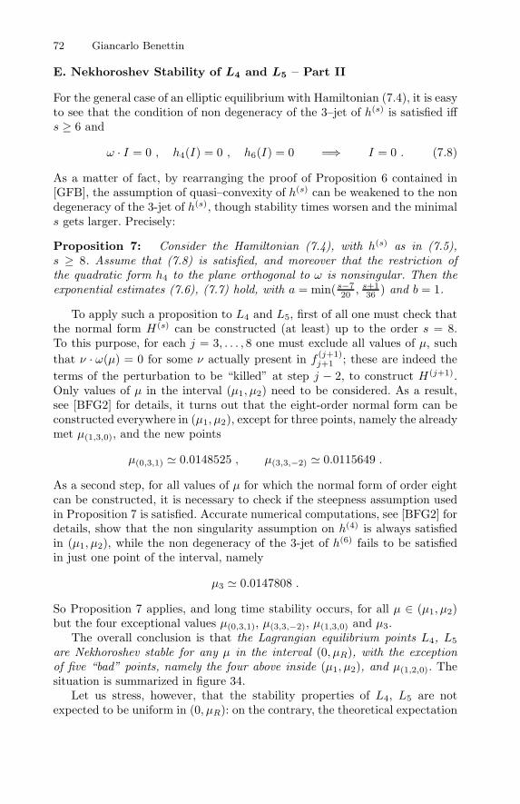
72 Giancarlo Benettin
E. Nekhoroshev Stability of L4 and L5 – Part II
For the general case of an elliptic equilibrium with Hamiltonian (7.4), it is easyto see that the condition of non degeneracy of the 3–jet of h(s) is satisfied iffs ≥ 6 and
ω · I = 0 , h4(I) = 0 , h6(I) = 0 =⇒ I = 0 . (7.8)
As a matter of fact, by rearranging the proof of Proposition 6 contained in[GFB], the assumption of quasi–convexity of h(s) can be weakened to the nondegeneracy of the 3-jet of h(s), though stability times worsen and the minimals gets larger. Precisely:
Proposition 7: Consider the Hamiltonian (7.4), with h(s) as in (7.5),s ≥ 8. Assume that (7.8) is satisfied, and moreover that the restriction ofthe quadratic form h4 to the plane orthogonal to ω is nonsingular. Then theexponential estimates (7.6), (7.7) hold, with a = min( s−7
20 ,s+136 ) and b = 1.
To apply such a proposition to L4 and L5, first of all one must check thatthe normal form H(s) can be constructed (at least) up to the order s = 8.To this purpose, for each j = 3, . . . , 8 one must exclude all values of µ, suchthat ν · ω(µ) = 0 for some ν actually present in f
(j+1)j+1 ; these are indeed the
terms of the perturbation to be “killed” at step j − 2, to construct H(j+1).Only values of µ in the interval (µ1, µ2) need to be considered. As a result,see [BFG2] for details, it turns out that the eight-order normal form can beconstructed everywhere in (µ1, µ2), except for three points, namely the alreadymet µ(1,3,0), and the new points
µ(0,3,1) 0.0148525 , µ(3,3,−2) 0.0115649 .
As a second step, for all values of µ for which the normal form of order eightcan be constructed, it is necessary to check if the steepness assumption usedin Proposition 7 is satisfied. Accurate numerical computations, see [BFG2] fordetails, show that the non singularity assumption on h(4) is always satisfiedin (µ1, µ2), while the non degeneracy of the 3-jet of h(6) fails to be satisfiedin just one point of the interval, namely
µ3 0.0147808 .
So Proposition 7 applies, and long time stability occurs, for all µ ∈ (µ1, µ2)but the four exceptional values µ(0,3,1), µ(3,3,−2), µ(1,3,0) and µ3.
The overall conclusion is that the Lagrangian equilibrium points L4, L5
are Nekhoroshev stable for any µ in the interval (0, µR), with the exceptionof five “bad” points, namely the four above inside (µ1, µ2), and µ(1,2,0). Thesituation is summarized in figure 34.
Let us stress, however, that the stability properties of L4, L5 are notexpected to be uniform in (0, µR): on the contrary, the theoretical expectation
Physical Applications of Nekhoroshev Theorem 73
is that the stability times worsen in the interval (µ1, µ2), where the assumptionof directional quasi–convexity is violated, and of course further worsen if theexceptional points where the theory fails are approached. As is remarkable,the value µEM relative to the Earth–Moon problem lies inside the intervalof weaker stability (µ1, µ2), and moreover, see figure 34, it is rather closeto µ(3,3,−2). As is known, no bodies have been ever observed to gravitatearound the triangular Lagrangian equilibria of the Earth–Moon system. Ofcourse, there can be several reasons for such an absence, like the (ratherstrong) influence of the Sun [GJMS], or the ellipticity of the underlying twobody problem. The worse stability of the ideal circular three body problem,however, could also contribute.
Whether the difference in the geometric properties of the system, namelyquasi–convexity or weaker steepness properties, does effectively result in ob-servable differences of the stability properties, is a very general question, whichgoes far beyond L4 and L5, or elliptic equilibria, and concerns the wholeNekhoroshev theory. Nekhoroshev, in his 1977 paper, explicitly conjecturedthat different steepness properties should lead to numerically observable dif-ferences in the stability times. Such a study, as is known, is not easy, sinceit based, in the essence, on the possibility of observing numerically, for smallperturbations, the Arnol’d diffusion — a quite difficult task, as is well known— and of putting in evidence possible differences in its speed. It is hard tosay whether such an investigation can be effectively carried on. But certainly,the Hamiltonian of L4, L5 provides, at least, a promising candidate for such astudy, since by just varying a natural parameter in the system, the steepnessproperties change significantly, and occasionally also disappear.
References
[A] H. Andoyer, Cours de Mechanique Celeste (Gautier-Villars, Paris 1923).[B] G. Benettin, Nekhoroshev-like Results for Hamiltonian Dynamical Sys-
tems, lectures given at the Noto School Non-Linear Evolution and ChaoticPhenomena, G. Gallavotti and P.W Zweifel Editors (Plenum Press, NewYork, 1988).
[BCaF] G. Benettin, A. Carati and F. Fasso, On the conservation of adiabaticinvariants for a system of coupled rotators. Physica D 104, 253–268 (1997).
[BCS] G. Benettin, A. Carati and P. Sempio, On the Landau–Teller ap-proximation for the energy exchanges with fast degrees of freedom.Journ. Stat. Phys. 73, 175–192 (1993).
[BCG] G. Benettin, A. Carati e G. Gallavotti, A rigorous implementation of theLandau–Teller approximation for adiabatic invariants. Nonlinearity 10,479-505 (1997).
[BChF1] G. Benettin, A.M. Cherubini and F. Fasso, A “changing chart” symplecticalgorithm for rigid bodies and other Hamiltonian systems on manifolds.SIAM Journ. on Sc. Computing 23, 1189–1203 (2001).
74 Giancarlo Benettin
[BChF2] G. Benettin, A.M.Cherubini e F. Fasso, Regular and Chaotic motions ofthe fast rotating rigid body: a numerical study. Discr. Cont. Dyn. Sys. 4,521–540 (2002).
[BF1] G. Benettin and F. Fasso, From Hamiltonian perturbation theory to sym-plectic integrators, an back. Appl. Num. Math. 29, 73-87 (1999).
[BF2] G. Benettin e F. Fasso, Fast rotations of the symmetric rigid body: a gen-eral study by Hamiltonian perturbation theory. Part I. Nonlinearity 9, 137–186 (1996).
[BFG1] G. Benettin, F. Fasso and M. Guzzo, Fast rotations of the symmetricrigid body: a study by Hamiltonian perturbation theory. Part II, Gyroscopicrotations. Nonlinearity 10, 1695–1717 (1997).
[BFG2] G. Benettin, F. Fasso and M. Guzzo, Nekhoroshev–stability of L4 and L5in the spatial restricted three-body problem. Regular and Chaotic Dynamics3, 56-72 (1998).
[BGa] G. Benettin and G. Gallavotti, Stability of Motions near Resonances inQuasi Integrable Hamiltonian Systems. Journ. Stat. Phys. 44, 293 (1986).
[BGi] G. Benettin and A. Giorgilli, On the Hamiltonian interpolation of near tothe identity symplectic mappings, with application to symplectic integrationalgorithms. Journ. Stat. Phys. 73, 1117–1144 (1994).
[BGG1] G. Benettin, L. Galgani e A. Giorgilli, Realization of Holonomic Con-straints and Freezing of High Frequency Degrees of Freedom, in the Lightof Classical Perturbation Theory. Part I. Comm. Math. Phys. 113, 87-103(1987).
[BGG2] G. Benettin, L. Galgani and A. Giorgilli, Realization of Holonomic Con-straints and Freezing of High–Frequency Degrees of Freedom in the Light ofClassical Perturbation Theory. Part II. Comm. Math. Phys. 121, 557-601(1989).
[BGG3] G. Benettin, L .Galgani e A. Giorgilli, A Proof of Nekhoroshev Theoremfor Nearly-Integrable Hamiltonian Systems. Celestial Mechanics 37, 1-25(1985).
[BHS] G. Benettin, P. Hjorth and P. Sempio, Exponentially long equilibrium timesin a one dimensional collisional model of a classical gas. Journ. Stat. Phys.94, 871-892 (1999).
[Bo1] L. Boltzmann, On certain questions of the theory of gases. Nature 51, 413(1895).
[Bo2] L. Boltzmann, Vorlesungen uber Gastheorie, Vol II, Section 45 (Barth,Leipzig 1898). English translation: Lectures on gas theory (University ofCal. Press, 1966).
[BS] G. Benettin and P. Sempio, Adiabatic invariants and trapping of pointcharge in a strong non–uniform magnetic field. Nonlinearity 7, 281–303(1994).
[D] A. Deprit, Free rotation of a rigid body studied in phase plane. Am. J.Phys. 55, 424 (1967).
[DGJS] A. Delshalms, V. Gelfreich, A. Jorba and T. M. Seara, Exponen-tially small splitting of separatrices under fast quasiperiodic forcing.Comm. Math. Phys. 189, 35–71 (1997).
[E] L.H. Eliasson, Absolutely convergent series expansions for quasi–periodicmotions. Math. Phys. Electronic J. 2, paper 4, 33 pp. (1996).
[F1] F. Fasso, Lie series method for vector fields and Hamiltonian perturbationtheory, J. Appl. Math. Phys. (ZAMP) 41, 843–864 (1990).
Physical Applications of Nekhoroshev Theorem 75
[F2] F. Fasso, The Euler–Poinsot top: a non-commutatively integrable systemwithout global action–angle coordinates. J. Appl. Math. Phys. 47, 953-976(1996).
[F3] F. Fasso, Hamiltonian perturbation theory on a manifold. Cel. Mech. andDyn. Astr. 62, 43–69 (1995).
[FGB] F. Fasso, M. Guzzo e G. Benettin, Nekhoroshev-stability of elliptic equi-libria of Hamiltonian systems. Comm. Math. Phys. 197, 347–360 (1998).
[Ga1] G. Gallavotti, Quasi–Integrable Mechanical Systems, in Critical phenom-ena, Random Systems, Gauge Theories, K. Osterwalder and R. Stora edi-tors, Les Houches, Session XLIII, 1984 (North–Holland, Amsterdam 1986).
[Ga2] G. Gallavotti, Twistless KAM tori, quasi flat homoclinic intersections,and other cancellations in the perturbation series of certain completelyintegrable hamiltonian systems. A review. Reviews Math. Phys. 6, 343–411 (1994).
[GDFGS] A. Giorgilli, A. Delshams, E. Fontich, L. Galgani e C. Simo, EffectiveStability for a Hamiltonian System near an Elliptic Equilibrium Point,with an Application to the Restricted three Body Problem. J. Diff. Eq. 77,167-198 (1989).
[GFB] M. Guzzo, F. Fasso e G. Benettin, On the stability of elliptic equilibria.Math. Phys. Electronic J. 4, paper 1, 16 pp. (1998).
[GG] A. Giorgilli and G. Galgani, Rigorous estimates for the series expansionsof Hamiltonian perturbation theory. Celestial Mech. 37 95–112 (1985).
[Gi1] A. Giorgilli, Rigorous results on the power expansions for the integrals ofa Hamiltonian system near an elliptic equilibrium point. Ann. Inst. HenriPoincare - Physique Theorique 48, 423–439 (1988).
[Gi2] A. Giorgilli, On the problem of stability for near to integrable Hamiltoniansystems. Proceedings of the International Congress of Mathematicians,Vol. III (Berlin, 1998).
[GJMS] G. Gomez, A. Jorba, J. Masdemont and C. Simo, A quasiperiodic solutionas a substitute of L4 in the Earth-Moon system. In: Predictability, stability,and chaos in N-body dynamical systems (Cortina d’Ampezzo, 1990), 433–438, NATO Adv. Sci. Inst. Ser. B Phys., 272 (Plenum, New York, 1991).
[GM] M. Guzzo e A. Morbidelli, Construction of a Nekhoroshev like result forthe asteroid belt dynamical system. Cel. Mech. & Dyn. Astr. 66, 255-292(1997).
[GS] A. Giorgilli and C.H. Skokos, On the stability of the Trojan asteroids,Astronomy and Astrophysics 317, 254-261 (1997).
[Gu] M. Guzzo, Nekhoroshev stability of quasi–integrable degenerate Hamilto-nian Systems. Regular and Chaotic Dynamics 4, 78-102 (1999).
[J1] J.H. Jeans, On the vibrations set up in molecules by collisions. Phil. Mag.6, 279 (1903).
[J2] J.H. Jeans, On the partition of energy between matter and Aether. Phil.Mag. 10, 91 (1905).
[J3] J.H. Jeans, The dynamical theory of gases, second edition, Chapter XIV.Cambridge Univ. Press (Cambridge, 1916).
[Li] J.E. Littlewood, Proc. London Math. Soc. 9, 343 (1959); 9, 525 (1959).[LN] P. Lochak e A.I. Neishtadt, Estimates of stability time for nearly integrable
systems with a quasiconvex Hamiltonian. Chaos 2, 495–499 (1992).[Lo1] P. Lochak, Canonical perturbation theory via simultaneous approximation.
Russ. Math. Surv. 47, 57-133 (1992).
76 Giancarlo Benettin
[Lo2] P. Lochak, Stability of Hamiltonian systems over exponentially long times:the near linear case. In H. Dumas, K. Meyer, D. Schmidt (eds), Hamilto-nian Dynamical Systems – History, Theory, and Applications, The IMAVolumes in Mathematics and its Applications 63, 221-229 (Springer, NewYork, 1995).
[LT] L. Landau and E. Teller, On the theory of sound dispersion. Physik. Z.Sowjetunion 10, 34 (1936). Also in Collected Papers of L. D. Landau,edited by D. Ter Haar, page 147 (Pergamon Press, Oxford 1965).
[MG] A. Morbidelli e M. Guzzo, The Nekhoroshev theorem and the Asteroid Beltdynamical system. Cel. Mech. & Dyn. Astr. 65, 107-136 (1997).
[NL] A.I. Neishtadt and M.L. Lidov, The method of canonical transformationsin problems of the rotation of celestial bodies and Cassini laws (Russian).In Determination of the motion of spacecraft (Russian), pag. 74–106 (Iz-dat. ”Nauka”, Moscow, 1975).
[Nei] A.I. Neishtadt, On the accuracy of conservation of the adiabatic invariant,Prikl. Mat. Mekh. 45:1, 80-87 (1981) [J. Appl. Math. Mech. 45:1, 58-63(1982)]
[Nek1] N.N. Nekhoroshev, Behaviour of Hamiltonian systems close to integrabil-ity. Funct. Anal. Appl. 5, 338-339 (1971) [Funk. An. Ego Prilozheniya, 5,82-83 (1971)].
[Nek2] N.N. Nekhoroshev, An exponential estimate of the time of stability ofnearly integrable Hamiltonian systems. Usp. Mat. Nauk 32:6, 5-66 (1977)[Russ. Math. Surv. 32:6, 1-65 (1977)].
[Ni1] L. Niederman, Nonlinear stability around an elliptic equilibrium point inan Hamiltonian system. Nonlinearity 11 1465–1479 (1998).
[Ni2] L. Niederman, Exponential stability for small perturbations of steep inte-grable dynamical systems. Erg. Theory Dyn. Sys. 2, 593-608 (2004).
[OH] T.M. O’Neil, P.G. Hjorth, Collisional dynamics of a strongly magnetizedpure electron plasma. Physics of Fluids 28, 3241, (1985).
[OHBFM] T.M. O’Neil, P.G. Hjorth, B. Beck, J. Fajans, and J. Malmberg, in Colli-sional relaxation of a strongly magnetized pure electron plasma (theory andexperiment). In Strongly Coupled Plasma Physics (North-Holland, Ams-terdam 1990).
[Po1] H. Poincare, Les Methodes Nouvelles de la Mechanique Celeste, Vol. 1(Gautier–Villars, Paris, 1892).
[Po1] J. Poschel, Nekhoroshev estimates for quasi–convex Hamiltonian Systems,Math. Z. 213, 187–216 (1993).
[Po2] J. Poschel, On Nekhoroshev’s estimate at an elliptic equilibrium. Internat.Math. Res. Notices 1999, no. 4, 203–215.
[Ra] D. Rapp, Complete classical Theory of Vibrational Energy exchange.Journ. Chem. Phys. 32, 735–737 (1960).
[Ru] R. Rutgers, Ann. Phys. 16, 350 (1933).[S] C. Simo, Averaging under fast quasiperiodic forcing. In Hamiltonian me-
chanics, integrability and chaotic behavior, J. Seimenis editor, Nato ASISeries B 331 (Plenum Press, New York 1994).
[SM] C. Siegel and J. Moser, Lectures on Celestial Mechanics (Springer, Berlin,1971).
The Adiabatic Invariant Theory andApplications
Jacques Henrard
Departement de Mathematique FUNDP 8,Rempart de la Vierge, B-5000 Namur, [email protected]
1 Integrable Systems
1.1 Hamilton-Jacobi Equation
We shall summarize in the section a few results of the theory of Hamiltoniansystem.
Canonical Transformations
By definition a canonical transformation from the phase space of n variables(q1, · · · , qn) and n momenta (p1, · · · , pn) to the phase space of n variables(β1, · · · , βn) and n momenta (α1, · · · , αn) is a (possibly time dependent)transformation such it transforms any Hamiltonian system into an Hamil-tonian system; i.e. for any function H(q, p) there exists a function K(β, α)such that the system of differential equations
qi =∂H
∂pi; pi = −∂H
∂qi1 ≤ i ≤ n ,
is transformed into the system of differential equations,
βi =∂H
∂αi; αi = −∂H
∂βi1 ≤ i ≤ n ,
A necessary and sufficient condition for a transformation to be canonicalis that its Jacobian matrix
M =∂(β1, · · · , βn, α1, · · · , αn)∂(q1, · · · , qn, p1, · · · , pn)
,
verify the condition
G. Benettin, J. Henrard, and S. Kuksin: LNM 1861, A. Giorgilli (Ed.), pp. 77–141, 2005.c© Springer-Verlag Berlin Heidelberg 2005
78 Jacques Henrard
MM = µ with =(
0n In−In 0n
)
,
where 0n is the (n×n) null matrix, and In is the (n×n) identity matrix. Whena transformation is canonical there exists a remainder function R(β, α, t) suchthat (
∂β/∂t∂α/∂t
)
=(
∂R/∂α−∂R/∂β
)
.
The “new” Hamiltonian K is equal to µH ′ +R , where H ′ is the functionH expressed in the “new” variables (β, α). A canonical transformation forwhich the multiplier µ is unity is a symplectic transformation.
A constructive method to generate symplectic transformation is the fol-lowing:
For any twice differentiable function S(q, α) such that the Hessian (∂2S/∂q∂α)is regular, the transformation from the phase space (q, p) to the phase space(β, α) implicitely defined by
pi =∂S
∂qi; βi =
∂S
∂αi1 ≤ i ≤ n ,
is a symplectic transformation.
Note that this is not the only way to construct symplectic transformationsand that not all symplectic transformations can be generated in this way.
Hamilton-Jacobi Equation
A function S(q, α) is a complete solution of the Hamilton-Jacoobi equationcorresponding to an Hamiltonian function H(q, p) if the functions (∂S/∂αi)are independent and if there exists a function K(α) such that
H(q1, · · · , qn,∂S
∂q1, · · · , ∂S
∂qn) = K(α1, · · · , αn) .
When we know a complete solution of Hamilton-Jacobi equation the Hamilto-nian system derived from H may be considered as solved. Indeed in the “new”phase space (β, α) the system is trivial. We have
αi = − ∂K∂βi
−→ αi = αi(0) ,βi = ∂K
∂αi= ni(α) −→ βi = nit+ βi(0) .
Of course, except in exceptional case the problem of finding a completesolution of Hamilton-Jacobi equation is at least as difficult as the problem ofsolving the original system of ordinary differential equations. A few of these“exceptional” cases are reviewed in the next section.
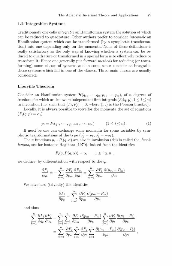
The Adiabatic Invariant Theory and Applications 79
1.2 Integrables Systems
Traditionnaly one calls integrable an Hamiltonian system the solution of whichcan be reduced to quadrature. Other authors prefer to consider integrable anHamiltonian system which can be transformed (by a symplectic transforma-tion) into one depending only on the momenta. None of these definitions isreally satisfactory as the only way of knowing whether a system can be re-duced to quadrature or transformed in a special form is to effectively reduce ortransform it. Hence one generally put forward methods for reducing (or trans-forming) some classes of systems and in some sense consider as integrablethose systems which fall in one of the classes. Three main classes are usuallyconsidered:
Liouville Theorem
Consider an Hamiltonian system H(q1, · · · , qn, p1, · · · , pn), of n degrees offreedom, for which are known n independant first integrals (Fi(q, p), 1 ≤ i ≤ n)in involution (i.e. such that (Fi;Fj) = 0, where (.; .) is the Poisson bracket).
Locally, it is always possible to solve for the momenta the set of equations(Fi(q, p) = αi)
pi = Pi(q1, · · · , qn, α1, · · · , αn) (1 ≤ i ≤ n) . (1)
If need be one can exchange some momenta for some variables by sym-plectic transformations of the type (q′k = pk, p
′k = −qk).
The n functions pi−Pi(q, α) are also in involution (this is called the Jacobilemma, see for instance Hagihara, 1970). Indeed from the identities
Fi(q, P (q, α)) = αi , 1 ≤ i ≤ n ,
we deduce, by differentiation with respect to the qk
∂Fi∂qk
= −n∑
m=1
∂Fi∂pm
∂Pm∂qk
=n∑
m=1
∂Fi∂pm
∂(pm − Pm)∂qk
.
We have also (trivially) the identities
∂Fi∂pk
=n∑
m=1
∂Fi∂pm
∂(pm − Pm)∂pk
.
and thusn∑
k=1
∂Fi∂qk
∂Fj∂pk
=n∑
k=1
n∑
m=1
∂Fi∂pm
∂(pm − Pm)∂pk
n∑
=1
∂Fj∂p
∂(p − P)∂pk
=n∑
m=1
∂Fi∂pm
n∑
=1
∂Fj∂p
n∑
k=1
∂(pm − Pm)∂pk
∂(p − P)∂pk
,
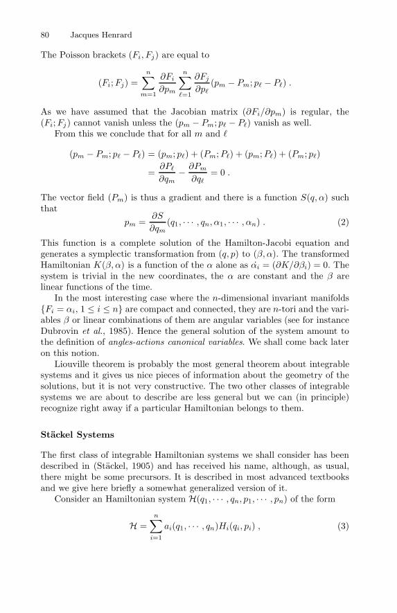
80 Jacques Henrard
The Poisson brackets (Fi, Fj) are equal to
(Fi;Fj) =n∑
m=1
∂Fi∂pm
n∑
=1
∂Fj∂p
(pm − Pm; p − P) .
As we have assumed that the Jacobian matrix (∂Fi/∂pm) is regular, the(Fi;Fj) cannot vanish unless the (pm − Pm; p − P) vanish as well.
From this we conclude that for all m and
(pm − Pm; p − P) = (pm; p) + (Pm;P) + (pm;P) + (Pm; p)
=∂P∂qm
− ∂Pm∂q
= 0 .
The vector field (Pm) is thus a gradient and there is a function S(q, α) suchthat
pm =∂S
∂qm(q1, · · · , qn, α1, · · · , αn) . (2)
This function is a complete solution of the Hamilton-Jacobi equation andgenerates a symplectic transformation from (q, p) to (β, α). The transformedHamiltonian K(β, α) is a function of the α alone as αi = (∂K/∂βi) = 0. Thesystem is trivial in the new coordinates, the α are constant and the β arelinear functions of the time.
In the most interesting case where the n-dimensional invariant manifoldsFi = αi, 1 ≤ i ≤ n are compact and connected, they are n-tori and the vari-ables β or linear combinations of them are angular variables (see for instanceDubrovin et al., 1985). Hence the general solution of the system amount tothe definition of angles-actions canonical variables. We shall come back lateron this notion.
Liouville theorem is probably the most general theorem about integrablesystems and it gives us nice pieces of information about the geometry of thesolutions, but it is not very constructive. The two other classes of integrablesystems we are about to describe are less general but we can (in principle)recognize right away if a particular Hamiltonian belongs to them.
Stackel Systems
The first class of integrable Hamiltonian systems we shall consider has beendescribed in (Stackel, 1905) and has received his name, although, as usual,there might be some precursors. It is described in most advanced textbooksand we give here briefly a somewhat generalized version of it.
Consider an Hamiltonian system H(q1, · · · , qn, p1, · · · , pn) of the form
H =n∑
i=1
ai(q1, · · · , qn)Hi(qi, pi) , (3)
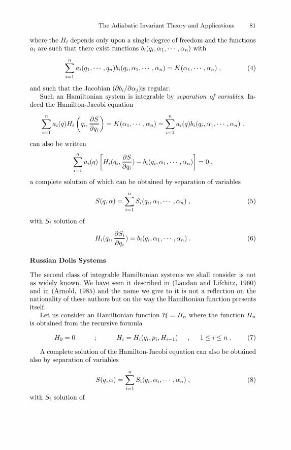
The Adiabatic Invariant Theory and Applications 81
where the Hi depends only upon a single degree of freedom and the functionsai are such that there exist functions bi(qi, α1, · · · , αn) with
n∑
i=1
ai(q1, · · · , qn)bi(qi, α1, · · · , αn) = K(α1, · · · , αn) , (4)
and such that the Jacobian (∂bi/∂αj)is regular.Such an Hamiltonian system is integrable by separation of variables. In-
deed the Hamilton-Jacobi equation
n∑
i=1
ai(q)Hi
(
qi,∂S
∂qi
)
= K(α1, · · · , αn) =n∑
i=1
ai(q)bi(qi, α1, · · · , αn) .
can also be writtenn∑
i=1
ai(q)[
Hi(qi,∂S
∂qi)− bi(qi, α1, · · · , αn)
]
= 0 ,
a complete solution of which can be obtained by separation of variables
S(q, α) =n∑
i=1
Si(qi, α1, · · · , αn) , (5)
with Si solution of
Hi(qi,∂Si∂qi
) = bi(qi, α1, · · · , αn) . (6)
Russian Dolls Systems
The second class of integrable Hamiltonian systems we shall consider is notas widely known. We have seen it described in (Landau and Lifchitz, 1960)and in (Arnold, 1985) and the name we give to it is not a reflection on thenationality of these authors but on the way the Hamiltonian function presentsitself.
Let us consider an Hamiltonian function H = Hn where the function Hn
is obtained from the recursive formula
H0 = 0 ; Hi = Hi(qi, pi, Hi−1) , 1 ≤ i ≤ n . (7)
A complete solution of the Hamilton-Jacobi equation can also be obtainedalso by separation of variables
S(q, α) =n∑
i=1
Si(qi, αi, · · · , αn) , (8)
with Si solution of
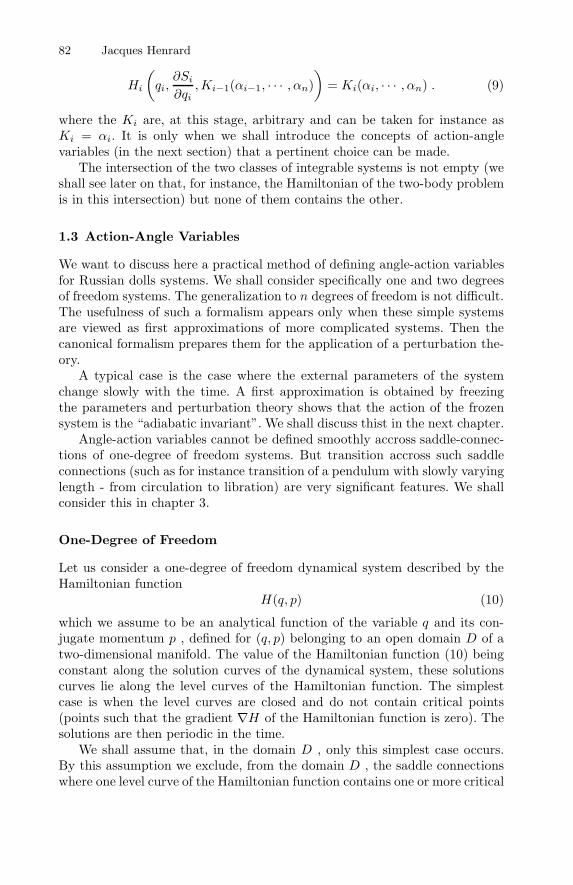
82 Jacques Henrard
Hi
(
qi,∂Si∂qi
,Ki−1(αi−1, · · · , αn))
= Ki(αi, · · · , αn) . (9)
where the Ki are, at this stage, arbitrary and can be taken for instance asKi = αi. It is only when we shall introduce the concepts of action-anglevariables (in the next section) that a pertinent choice can be made.
The intersection of the two classes of integrable systems is not empty (weshall see later on that, for instance, the Hamiltonian of the two-body problemis in this intersection) but none of them contains the other.
1.3 Action-Angle Variables
We want to discuss here a practical method of defining angle-action variablesfor Russian dolls systems. We shall consider specifically one and two degreesof freedom systems. The generalization to n degrees of freedom is not difficult.The usefulness of such a formalism appears only when these simple systemsare viewed as first approximations of more complicated systems. Then thecanonical formalism prepares them for the application of a perturbation the-ory.
A typical case is the case where the external parameters of the systemchange slowly with the time. A first approximation is obtained by freezingthe parameters and perturbation theory shows that the action of the frozensystem is the “adiabatic invariant”. We shall discuss thist in the next chapter.
Angle-action variables cannot be defined smoothly accross saddle-connec-tions of one-degree of freedom systems. But transition accross such saddleconnections (such as for instance transition of a pendulum with slowly varyinglength - from circulation to libration) are very significant features. We shallconsider this in chapter 3.
One-Degree of Freedom
Let us consider a one-degree of freedom dynamical system described by theHamiltonian function
H(q, p) (10)
which we assume to be an analytical function of the variable q and its con-jugate momentum p , defined for (q, p) belonging to an open domain D of atwo-dimensional manifold. The value of the Hamiltonian function (10) beingconstant along the solution curves of the dynamical system, these solutionscurves lie along the level curves of the Hamiltonian function. The simplestcase is when the level curves are closed and do not contain critical points(points such that the gradient ∇H of the Hamiltonian function is zero). Thesolutions are then periodic in the time.
We shall assume that, in the domain D , only this simplest case occurs.By this assumption we exclude, from the domain D , the saddle connectionswhere one level curve of the Hamiltonian function contains one or more critical
The Adiabatic Invariant Theory and Applications 83
points and orbits asymptotic to these critical points. We shall comment onthe saddle connections in chapter 3. We exclude also the cases where the levelcurves and the orbits extend to infinity. These orbits are usually not veryinteresting candidates for a perturbation theory.
In summary, we assume that D is
1. an open, bounded invariant set,2. does not contain critical points.
The extension to a domain containing a single stable equilibrium point isnot difficult but necessitates some special discussions that we prefer to avoidhere.
In such a domain D , the general solution of the dynamical system de-scribed by the Hamiltonian (10) can be written
q = Q(t, h)p = P (t, h) (11)
where the functions P,Q are periodic in the time t of period T (h) . Theparameter h is the value of the Hamiltonian function. In writing the generalsolution (11) we have assumed that an initial point (corresponding to t = 0 )has been chosen on each solution curve by taking q0 = Q(0, h) and p0 =P (0, h) on a curve defined by an analytical function
F (q0, p0) = 0 . (12)
This curve should of course intercept transversaly all the solutions in thedomain D .
Our aim, in this section, is to write the general solution (11) under theform of a canonical transformation:
q = Q(ψ, J)p = P (ψ, J) (13)
from an angular variable ψ (increasing by 2π along each closed solution curve)and an action J , its conjugate momentum, which will obviously take the roleof h in labelling each solution curve. This will be done by defining ψ and Jas functions of t and h .
An obvious choice is to define ψ as a normalized time
ψ =2πT (h)
t (14)
and to find the function h(J) which makes
Q(ψ, J) = Q(T (h(J))
2πψ, h(J))
P (ψ, J) = P (T (h(J))
2πψ, h(J))
84 Jacques Henrard
a canonical transformation. We have to check
(Q;P ) =∂Q
∂ψ
∂P
∂J− ∂Q
∂J
∂P
∂ψ
=T
2π∂h
∂J
∂Q
∂t
∂P
∂h− ∂Q
∂h
∂P
∂t
= 1 (15)
When we substitute to ∂Q∂t and ∂P
∂t the right-hand members of the Hamil-tonian differential equations, the condition (15) becomes
(Q;P ) =T
2π∂h
∂J
∂H
∂p
∂P
∂h+∂H
∂q
∂Q
∂h
= 1 . (16)
But from the identity
H(Q(t, h), P (t, h)) = h (17)
it is easy to conclude that the expression in brackets in (16) is equal to oneand thus that the unknown function h(J) is defined implicitely as the solutionof
∂J
∂h=T (h)2π
. (18)
Equation (18) is also of course a definition of the action variable J . Thisdefinition can be written under a form from which its geometrical meaning ismade more apparent.
The following identity is not difficult to check
∂
∂J
∂Q
∂ψP − ∂P
∂ψQ
= 2(Q;P ) +∂
∂ψ
∂Q
∂JP − ∂P
∂JQ
.
By integrating both members with respect to ψ , we find:
∂
∂J
∫ 2π
0
∂Q
∂ψP − ∂P
∂ψQ
dψ = 4π +[∂Q
∂JP − ∂P
∂JQ]2π
0
. (19)
The last term in (19) disappears as the functions P , Q are 2π-periodic inψ . Hence we find that, up to an arbitrary additive constant, the action J isequal to:
J =14π
∫ 2π
0
∂Q
∂ψP − ∂P
∂ψQ
dψ (20)
or equivalently to
J =14π
∫ T
0
∂Q
∂tP − ∂P
∂tQ
dt
orJ =
14π
∮
pdq − qdp (21)
The Adiabatic Invariant Theory and Applications 85
where the path integral (21) is taken along the closed solution curve.The last expression makes it obvious that 2πJ can be usually defined
geometrically as the area enclosed by the solution curve. We say usually be-cause in some instances, the closed solution curve does not enclose a finitearea (for instance when the closed solution curve goes around a cylinder). Inthese cases, the expression (21) is still well-defined and related to an area, butshould receive another geometrical interpretation. Notice also that the areawe are talking about is an oriented area. The direction of motion along thesolution curve defines the sign of J .
In most textbooks the canonical transformation to action-angle variablesis not defined in the same way but rather by means of the mixed generat-ing function and the Hamiltonian-Jacobi equation. This other definition isequivalent and indeed may seem simpler. We did not follow the traditionalpresentation because the implicit character of the mixed generating functionhides most of the topological difficulties of the problem. Let us sketch anywaythis usual presentation.
Let us assume that the canonical transformation (13) is defined implicitelyby the mixed generating function S(q, J):
p =∂S
∂Q, ψ =
∂S
∂J(22)
and let us assume that it is such that the Hamiltonian function H(q, p) istransformed into a function K(J) of J alone. The corresponding Hamilton-Jacobi equation is:
H(q,∂S
∂q) = K(J) (23)
and its solution is given by
S(q, J) =∫ q
q0
P(q′,K(J)) dq′ (24)
where the function P(q, h) is defined implicitely by the identity
H(q,P(q, h)) = h .
Notice that the implicit function P may not be unique and that the integraldefining S is actually a path-integral. For instance in the case of the pendulum
H =12p2 − b cos q
there is an ambiguity in the definition of the function P
P = ±√
2h+ 2b cos q
which must be solved in connection with the definition of the path integral(24). P is positive when q is increasing and P is negative when q is decreasing
86 Jacques Henrard
along the solution. Such difficulties do not arise with the explicit definitionwe have chosen. Setting aside those difficulties, we observe that from thedefinition of the canonical transformation:
ψ =∂S
∂J=∂K
∂J
∫ q
q0
∂P∂h
dq ,
if we assume that q0 does not depend upon h. If we cannot, or do not wish, tomake this assumption, the computation becomes much more involved.
If we want the variable ψ to be an angular variable, increasing by 2π aftera complete circuit along the periodic orbit, we should have
2π =∂K
∂J
∂
∂h
∮
P(q, h) dq
and thus, up to an additive constant,
J(h) =12π
∮
P(q, h) dq
which is equivalent to (21).
Two Degree of Freedom Separable Systems
A n-degree of freedom separable system is in some sense a juxtaposition ofn one-degree of freedom systems, with minimal interaction between them. Itwould then seems enough to develop the one-dimensional case as we just did.Nevertheless there are a few particular points worth mentionning. Let us theninvestigate with more details the case of a two-degree of freedom system. Theextension to n-degree of freedom is straightforward although the notationsmay become clumsy.
Let us consider a Russian doll system with two degrees of freedom
H(q1, p1, L(q2, p2)) . (25)
The differential equations corresponding to the second degree of freedom
q2 =∂H
∂L
∂L
∂p2, p2 = −∂H
∂L
∂L
∂q2
can be viewed as a one-degree of freedom system
dq2dτ
=∂L
∂p2,
dp2
dτ= − ∂L
∂q2(26)
in the “pseudo-time”
τ =∫ t
0
(∂H
∂L) dt . (27)
The Adiabatic Invariant Theory and Applications 87
Notice that the “pseudo-time” τ does depend upon the first degree of freedom,but except for this, the system (26) is separated from this first degree offreedom.
If we assume that the solutions of (26) are periodic in τ of period T2(L)in a domain of the phase space (q2, p2) , we can introduce in this domainaction-angle variables
ϕ2 = 2πT2τ
J2 =∮
p2dq2 − q2dp2(28)
as we have done in the previous section. The transformation from (ϕ2, J2) to(q2, p2) given by
q2 = Q2(ϕ2, J2)p2 = P 2 (ϕ2, J2)
(29)
is a one-degree of freedom canonical transformation, which completed by theidentity transformation for the first degree of freedom, transforms the Hamil-tonian (25) into
M(q1, p1, J2) (30)
where J2 is a constant. If we consider the Hamiltonian (30) as a one-degree offreedom Hamiltonian in (q1, p1) depending upon a parameter J2 , and if thesolutions of the system described by (30) are periodic of period T1(M) in adomain of the phase space (q1, p1) , it is natural to introduce the action-anglevariables
ψ1 = 2πT1t
J1 =∮
p1dq1 − q1dp1(31)
by means of the one-degree of freedom canonical transformation, dependingupon the parameter J2:
q1 = Q1(ψ1, J1, J2)p1 = P 1 (ψ1, J1, J2)
(32)
The question is now: can we make out of the two one-degree of freedomcanonical transformations (29) and (32), one two-degree of freedom canonicaltransformation ?
To answer this question, we shall need, as we shall see, to distinguish inthe scaled “pseudo-time” ϕ2 a mean value, which will be used as the angularvariable ψ2 of the action-angle pair, and a periodic correction (ψ1, J1, J2)which will take into account the periodic variations of the “pseudo-time” withthe motion of the first degree of freedom.
Let us first juxtapose the transformations (29) and (32) but, while doingso, let us give us some freedom by allowing us the possibility of correcting thedefinition of the angle variable ψ2 in terms of ϕ2 . We shall see later on thatthis correction is the one we just mentioned.
q1 = Q1(ψ1, J1, J2)p1 = P 1 (ψ1, J2, J2)q2 = Q2(ψ2 + , J2)p3 = P 2 (ψ2 + , J2)
(33)
88 Jacques Henrard
The “correction” is assumed to be a yet unknown function of (ψ1, J1, J2) .It is a matter of a little algebra to verify that the Poisson bracket conditions
of canonicity:
(Qi ;Pj ) = δij , (Qi ;Q
j ) = (P i ;P j ) = 0
amounts to the following partial differential equations for the unknown func-tion :
∂
∂ψ1=∂Q1∂J2
∂P 1∂ψ1
− ∂Q1∂ψ1
∂P 1∂J2
∂
∂J1=∂Q1∂J2
∂P 1∂J1
− ∂Q1∂J1
∂P 1∂J2
(34)
The Froebenius condition of integrability of this set of partial differentialequations reduce after some algebra to the condition
∂
∂J2
[∂Q1∂ψ1
∂P 1∂J1
− ∂Q1∂J1
∂P 1∂ψ1
]
= 0
which is obviously verified in view of the fact that the transformation (32) is aone-degree of freedom canonical transformation. Hence the partial differentialequations (34) can be integrated and yield
=∫ ψ1
0
[∂Q1∂J2
∂P 1∂ψ1
− ∂Q1∂ψ1
∂P 1∂J2
]
dψ1 +∫ J1
G(J1, J2) dJ1 (35)
where the function G(J1, J2) is defined as
G(J1, J2) =[∂Q1∂J2
∂P 1∂J1
− ∂Q1∂J1
∂P 1∂J2
]
ψ1=0
.
We have mentioned that the correction (ψ1, J1, J2) which we have justevaluated, can be viewed as a description of the relationship between the“pseudo-time” τ (see (27)) and the time t . Indeed we find easily that
dϕ2
dt=
2πT2
dτ
dt=dM
dJ2.
On the other hand, the time derivative of the angular variable ψ2 is given by
dψ2
dt=∂K
∂J2
where K is the Hamiltonian function expressed in the action variables
K(J1, J2) = M(Q1(ψ1, J1, J2), P 1 (ψ1, J1, J2), J2) . (36)
Differentiating the identity (36) with respect to J2 we find
The Adiabatic Invariant Theory and Applications 89
d
dt=dϕ2
dt− dψ2
dt= −∂M
∂q1
∂Q1∂J2
− ∂M
∂p1
∂P 1∂J2
which, by using the differential equations in q1 and p1 becomes
d
dt=∂Q1∂J2
∂P 1∂t− ∂Q1
∂t
∂P 1∂J2
. (37)
Considering the linear relationship between the time and ψ1 , (37) reproducesthe time derivative of (35). The second integral in (35) which gives the valueof at ψ1 = 0 , represents a “canonical synchronization” of the two timevariables ϕ2 and ψ2 .
From the fact that (ψ1, J1, J2) is, up to a scale factor, the differencebetween the “pseudo-time” variable ϕ2 and the uniform time variable ψ2 , wecan hope that actually ψ2 reproduces the mean value of the “pseudo-time”and the periodic corrections. This is indeed the case. To check it we recallthat J1 is defined as
J1 =14π
∫ 2π
0
P 1∂Q1∂ψ1
−Q1∂P 1∂ψ1
dψ1 .
Differentiating the identity with respect to J2 gives, after an integration bypart,
0 = (2π, J1, J2)− (0, J1, J2)−12
[
P 1∂Q1∂J2
−Q1∂P 1∂J2
]2π
0
.
Due to the periodicity of Q1, P1 with respect to ψ1 the last term disappears
and we conclude that is indeed 2π-periodic with respect to ψ1 .
2 Classical Adiabatic Theory
The Adiabatic Invariant
Let us consider an Hamiltonian function which depends upon a parameter λ
H(q, p, λ) (38)
and let us consider that this parameter λ varies slowly with the time. By thiswe mean not only that dλ/dt is small but that higher order derivatives of λare smaller yet, i.e. that there exists a small quantity ε such that
1n!
∣∣∣∣
dnλ
dtn
∣∣∣∣≤ εn . (39)
Our results will be valid for ε “sufficiently small”, i.e. they will be asymptoticresults. To simplify the notation we shall assume actually that
90 Jacques Henrard
λ = εt . (40)
This can be done without loss of generality. The assumption (39) or (40) mayseem to be strong but it is essential. It is not always quoted in full and issometime hidden in the naive picture (pleasantly recalled by Arnold, 1978)that the “devil” pulling the strings (i.e. making λ a function of the time) is notonly slow but ignores what the dynamical system does. Well, actually, he mayknow it but condition (39) makes him powerless to adjust to the dynamicalsystem.
For a small to moderate length of time, the trajectory of the dynamicalsystem described by (38) will not differ much from the trajectory of the “frozensystem”H(q, p, λ0) where λ has been “frozen” to its constant initial value λ0 =λ(0) . Later on, for a small interval of time around the value t , the trajectorieswill again be close to the trajectories of the system H(q, p, λ) frozen at adifferent value λ = λ(t) . For a small interval of time around any given timet , we can approximate the trajectory by its “guiding trajectory” which isdefined as the trajectory of the system frozen at this given time, with initialcondition (q(t), p(t)) . The problem addressed by the adiabatic invarianttheory is to describe the evolution with time of the guiding trajectory: Howdo we find at time t , the guiding trajectory of the trajectory starting atq0, p0 at time t = 0 .
To address this question we shall make use of course of the angle-actionvariables introduced in the previous chapter. But the transformation to angle-action variable now depends upon the parameter λ and thus upon the time
q = Q(ψ, J, λ)p = P (ψ, J, λ) (41)
We extend the phase space to (λ, q, Λ, p) , where λ is a scaled time variableand Λ its conjugate momentum, and replace the time dependent Hamilto-nian function H(q, p, εt) by a two-degree of freedom autonomous HamiltonianH(q, p, λ) + εΛ .
The one-degree of freedom canonical transformation (41) is extended to atwo-degree of freedom canonical transformation by
λ = λ′
Λ = Λ′ +R(ψ, J, λ′) (42)
where the remainder function R is given by the time derivative of the mixedgenerating function (24)
R = −∂S∂λ
or, if we want to avoid using this mixed generating function, by the expression
R =∫ ψ
0
(∂Q
∂ψ
∂P
∂λ− ∂Q
∂λ
∂P
∂ψ
)
dψ +∫ J (∂q0
∂J
∂p0
∂J− ∂q0∂J
∂p0
∂J
)
dJ
(43)
The Adiabatic Invariant Theory and Applications 91
which can be deduced from the symplectic condition. In any case we do notneed here to know the exact form of the remainder function R except for thefact that it is a periodic function of ψ .
The new Hamiltonian of the dynamical system is now
K ′ = K(J, λ′) + ε Λ′ +R(ψ, J, λ′) (44)
and it is a straightforward application of the classical perturbation theory togenerate a canonical transformation close to the identity
(ψ, λ′, J, Λ′) −→ (øψ, λ′, øJ, øΛ′) (45)
such that the new Hamiltonian function
øK = K(øJ, λ′) + ε øΛ′ + øR(øJ, λ′, ε)+ εn+1 Kr(øψ, øJ, λ′, ε) (46)
does not depend upon the angular variable ψ up to terms of order εn for agiven integer n .
To see this we just have to check that the vector space F of analyticalfunction of (ψ, J, λ) , periodic of period 2π in ψ is the direct sum of the vectorspace F1 of analytical function of (ψ, J, λ) with zero mean value in ψ and ofF2 the set of analytical function of (J, λ) . Furthermore, F1 belongs to theimage of F by the operator
(K; ·) = −(∂K
∂J
)∂
∂ψ
if ∂K∂J is different from zero. Notice that the function ∂K
∂J = 2πT will enter the
denominator at each step of the averaging procedure and thus that we haveto make sure that it is bounded away from zero uniformly in ε in order toinsure that the unaveraged remainder εnKr can be made as small as neededfor small values of ε . Hence the domain D(λ) on which we have defined theangle-action variables and now the averaged angle-action variables (øψ, øJ)should not contain a saddle connection in its closure.
The differential equation for the averaged action øJ is∣∣∣∣
døJdt
∣∣∣∣= εn+1
∣∣∣∣
∂Kr
∂ψ
∣∣∣∣= C1ε
n+1 (47)
where C1 is the supremum of |∂Kr
∂ψ | in the domain D(λ) .It can be used in a straightforward manner to evaluate the time-variation
of øJ :|øJ(t)− øJ(0)| ≤ C1ε
n+1t (48)
as long as the trajectory remains in the domain øD(λ) , where øD(λ) isthe image of D(λ) by the averaging transformation. It can be reduced to0 ≤ ψ ≤ 2π and øJmin(λ) ≤ øJ ≤ øJmax(λ) . Of course the constant C1 in(47) depends upon the order n and may get very large for large n .
92 Jacques Henrard
As we can monitor the variation of øJ by (48) itself, the estimate (48)is valid as long as one of the limit øJmin(λ) or øJmax(λ) does not approachøJ(0) or as long as |t| ≤ ε−n . Hence the estimate is valid for a very longtime ( |t| ≤ ε−n ) unless the trajectory is forced out of the domain D(J) ofdefinition of the action-angle variable by approaching, for instance, a saddle-connection.
The averaged action øJ is not immediately accessible, and its geometricalmeaning is somewhat blurred by the averaging procedure defining it. The non-averaged action J which differs from øJ by terms of the order of ε verify aweaker but perhaps more useful inequality:
|J(t)− J(0)| ≤ C2ε , for |t| ≤ ε−n (49)
unless of course the trajectory is forced out of the domain D(λ) before thistime. This is why the action is called an adiabatic invariant and how it an-swers the question we raised at the beginning of this section: At time t theguiding trajectory of the trajectory starting at q0, p0 at time t = 0 is thisguiding trajectory which admits the same action (labelled by the same valueJ ) than the starting guiding trajectory.
The non-averaged momentum J , the classical action-variable, can be ex-pressed as a function of the averaged variable (ψ, J) by means of the pertur-bation series. It leads to
J = J + εJn(ψ, J, λ, ε) (50)
where Jn is an analytical function periodic of period 2π in ψ. The first ordercontribution of Jn is easy to compute and will be useful later on. We have
J = J − ε(∂K
∂J
)−1
R(ψ, J , λ)− < R(ψ, J , λ) >+O(ε2) , (51)
where < · > stands for the averaged value over ψ. Inverting (51) we obtain:
J = J + ε
(∂K
∂J
)−1
R(ψ, J, λ)− < R(ψ, J, λ) >+O(ε2) . (52)
Applications
The Modulated Harmonic Oscillator
As a first example let us consider the modulated harmonic oscillator, theHamiltonian of which is
H(q, p) =12(
p2 + ω(λ)q2)
, (53)
The Adiabatic Invariant Theory and Applications 93
with λ = εt. The general solution is
q =
√2hω
sin(ωt) ,
p =√
2h cos(ωt .
We have choosen the line of initial conditions as q = 0. The period is 2π/ωfor all orbits. From formula (18) or from formula (21) we find
J =h
ω. (54)
Indeed one of the first mention of the principle of adiabatic invariance is aremark made by Einstein at one of the Solvay conference that changing slowlythe frequency of the oscillator will keep the action constant but change theenergy accordingly. This was an important remark in view of the fact thatin his mind the oscillator was a simplified model of an atom submitted to avarying magnetic field. The action should be quantified and thus could not“change slowly”.
The Two Body Problem
The central force problem to which the two body problem can be reduced, isdescribed in spherical coordinates by the Hamiltonian,
H(q, p) =1
2m
[
p2r +
1r2
(
p2ϑ +
p2ϕ
cos2 ϑ
)]
+m
r, (55)
This Hamiltonian is both a Stackel Hamiltonian and a “Russian doll” Hamilto-nian. It is thus integrable and it is well known that, in terms of the traditionalelliptic elements, the actions are
L =√ma , G =
√
ma(1− e2) , H =√
ma(1− e2) cos I , (56)
where a is the semi major axis, e the eccentricity, and I the inclination of theorbit.
Let us consider a slow variation of the mass m of the attracting center. Asthe actions are kept constant, it is an immediate conclusion that the shape ofthe orbit (given by the parameters e and I) stays constant but that the sizeof the orbit (the semi-major axis) varies as the inverse of the mass.
The Pendulum
Various physical problems of interest can be modelized by a pendulum withslowly varying parameters.
94 Jacques Henrard
The most obvious one is, of course, the pendulum itself with variable lengthλ(t):
H =12I2 − b(t) cosϕ with b = gL3 . (57)
Notice that we should not use the usual normalization y = pϕ/L2 which, from
the HamiltonianH ′ =
12p2ϕ / L
2 − gL cosϕ
leads to the Hamiltonian
H ′′ =12y2 − g
Lcosϕ .
Indeed, when λ is a function of time, the usual normalization is no longercanonical. Instead, we have used a change of time scale τ = t/λ2.
More generally, many resonance problems with variable restoring torquecan be modelized by (57).
On top of the (slow) variation of the restoring torque b(t) of the pendulum,one can take into account a (small) outside torque (−c) by considering thedifferential equation
ϕ = −b sinϕ− c . (58)
Defining the momentum I = ϕ+ c , one is led to the Hamiltonian function
H =12(I − c)2 − b cosϕ . (59)
In plasma physics, one considers particles moving in a wave field withslowly varying amplitude and phase velocity leading to the equation (see, forinstance, Caryet al., 1986)
ϕ = −b(t) sin(ϕ− d(t)) .
The equation for the angular variables ψ = ϕ− d is similar to (58) with creplaced by d. Hence we are led to (59) with c replaced by d.
Menyuk (1985) prefers to consider a two modes system
H =12I2 − α cos(ϕ− εt)− β cos(ϕ+ εt)
which can be put under the form (59) if we take
b sind = (α− β) sin εt ,b cosd = (α+ β) cos εt . (60)
The Adiabatic Invariant Theory and Applications 95
The equation for the synchroneous motor:
ϕ = −b0 sinϕ+ aϕ (61)
with a small dissipative term (aϕ) has been studied by Andronov et al. (1966)and Urabe (1954, 1955). Burns (1978) applied their results to the rotation ofMercury. This problem can also be modelized by the Hamiltonian (57). If wedefine the “momentum” I by
I = ϕe−at , (62)
and the new time variable τ by:
aτ = eat , (63)
we are led to the differential equations:
dϕ
dτ= I ,
dI
dτ= −e−2atb0 sinϕ = −(aτ)−2b0 sinϕ , (64)
which corresponds to the Hamiltonian (55) with b = b0e−2at = (aτ)−2b0.
It may seem strange that a dissipative problem like (61) is mapped ontoan Hamiltonian problem like (55). This apparent paradox is explained whenone considers that (62) is time dependent and thus that a conservation of areain the phase space (ϕ, I) corresponds to an exponential decrease in area inthe phase space (ϕ, ϕ).
From this brief review, it is obvious that the slowly varying pendulum canmodelize a large variety of interesting phenomena which all can be describedby the Hamiltonian function (59). We shall slightly modify its expression tohave h = 0 on the stable equilibrium and study the Hamiltonian function:
h =12(I − c)2 + 2b sin2 ϕ
2(65)
where b and c are slow functions of the time.
The action-angle variables (ψ, J) of the frozen system (65) are well-known.They are related to the variable (ϕ, I) by means of
In case of libration In case of circulation
α = h/2b < 1 β−1 = h/2b > 1
sinϕ/2 =√α sin sinϕ/2 = sinϑ
S = 4√b(α− 1)F(, α) + E(, α) + cϕ S = 4
√
b/βE(ϑ, β)· sgn (I − c) + cϕ
ψ = F(, α)π/2K(α) ψ = F(ϑ, β)(π/K(β))· sgn (I − c)
J = 8√b(α− 1)K(α) + E(α)/π J = 4
π
√
b/βE(β) + c sgn (I − c)
∂J/∂h = 2√bK(α)/π ∂J/∂h =
√
β/bK(β)/π
96 Jacques Henrard
The functions F(, α) , E(, α) , · · · are the usual elliptic integrals (seeAbramowitz and Stegun, 1965, for the notations) and Z(, α) which appearslater is the Jacobi’s zeta function.
What is a little less known, although it can be found under various forms,more or less explicit in Best (1968), Timofeev (1978), Menyuk (1985), arethe formulae for the slowly varying pendulum. One finds that the remainderfunction of the canonical transformation going from (ϕ, I) to (ψ, J) isin case of Libration:
εR = cϕ+2b√bZ(, α) ,
in case of Circulation:
εR =c
K(β)2K(β)ϑ− πF(ϑ, β) +
2bb
√
b/βZ(ϑ, β) .
In both cases, the mean value of the remainder function vanishes
< R >=12π
∫ 2π
0
R dψ = 0 .
From this, it is easy to compute the first order correction to the adiabaticinvariant. From (I.72), we obtainin case of Libration:
J = J +2πK(α)2b
bZ(, α) +
c√bϕ+O(
ε2 log2(α− 1)α− 1
) ,
in case of Circulation:
J = J +1πK(β)
2bb
Z(ϑ, β) + 2cϑ√
β/b
− cF(ϑ, β)√
β/b
+ O(ε2 log2(β − 1)
β − 1) .
The Magnetic Bottle
If the adiabatic invariance received prominence because of its role in the earlyformulation of quantum mechanics, its importance in classical mechanics be-came first of significance for applications in connection with the magneticmomentum of gyration of a charged particle in a strong magnetic field. Thiswas shown to be an invariant by Alfven (1950) in his investigation of cosmicalrays. Very soon afterwards, its usefulness in the theoretical design of devicesfor controlling hot plasmas (Stellarators, Tokamaks, Mirror Machines, · · · )
The Adiabatic Invariant Theory and Applications 97
was recognized (see, for instance, Kruskal, 1952; see also Freidberg, 1982 fora recent review).
We shall try in this section to suggest why the adiabatic invariance isso important in this context, without, of course, giving a full account of itstechnical applications. This would require by itself a complete review paperwhich we are not competent to write.
The motion of a particule of mass m and electric charge e in an electro-magnetic field is controled by the Hamiltonian function:
H =1
2m||p− e
cA(x)||2 + eϕ(x) (66)
where ϕ and A are respectively the electric potential and the magnetic vectorpotential of the field:
E = −grad ϕ ,B = rot A .
The vector x is the position vector of the particle and the vector p its mo-mentum related to its velocity V by
p = mV +e
cA . (67)
Let us assume that the vector-potential and the magnetic field are givenby
A = B0(1 + b(x3))x1e2 , (68)B = B0(1 + b)e3 −B0b
′x1e1 , (69)
where (x1, x2, x3) are the cartesian coordinates of x in an orthonormal basis(e1, e2, e3) and b′ is the first derivative of b with respect to x3.
This magnetic field describes a two-dimensional “magnetic bottle” (withtwo throats). The magnetic field is an almost constant field in the directionof e3 but slightly (if b′ is small) modulated. The magnetic lines are given by
x1 =x1(0)
1 + b(x3), x2 = x2(0) (70)
and their shape is illustrated in Figure 24 for b = β2x23.
It would have been more realistic to consider a magnetic field with cylin-drical symmetry described for instance by:
A =B0
2(1 + b)[x1e2 − x2e1] ,
B = B0(1 + b)e3 −B0b
′
2[x1e1 + x2e2]
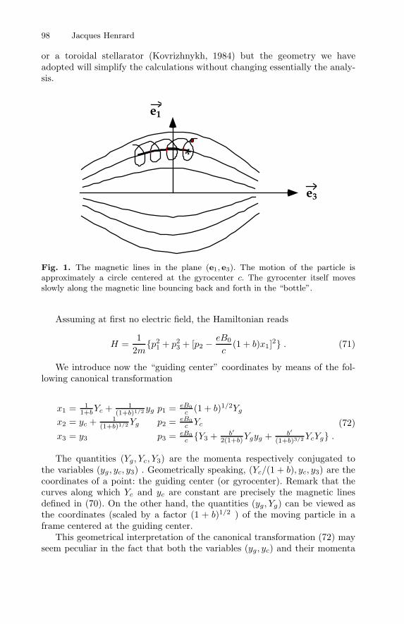
98 Jacques Henrard
or a toroidal stellarator (Kovrizhnykh, 1984) but the geometry we haveadopted will simplify the calculations without changing essentially the analy-sis.
*
e3
e1
Fig. 1. The magnetic lines in the plane (e1, e3). The motion of the particle isapproximately a circle centered at the gyrocenter c. The gyrocenter itself movesslowly along the magnetic line bouncing back and forth in the “bottle”.
Assuming at first no electric field, the Hamiltonian reads
H =1
2mp2
1 + p23 + [p2 −
eB0
c(1 + b)x1]2 . (71)
We introduce now the “guiding center” coordinates by means of the fol-lowing canonical transformation
x1 = 11+bYc + 1
(1+b)1/2 yg p1 = eB0c (1 + b)1/2Yg
x2 = yc + 1(1+b)1/2Yg p2 = eB0
c Yc
x3 = y3 p3 = eB0c Y3 + b′
2(1+b)Ygyg + b′(1+b)3/2YcYg .
(72)
The quantities (Yg, Yc, Y3) are the momenta respectively conjugated tothe variables (yg, yc, y3) . Geometrically speaking, (Yc/(1 + b), yc, y3) are thecoordinates of a point: the guiding center (or gyrocenter). Remark that thecurves along which Yc and yc are constant are precisely the magnetic linesdefined in (70). On the other hand, the quantities (yg, Yg) can be viewed asthe coordinates (scaled by a factor (1 + b)1/2 ) of the moving particle in aframe centered at the guiding center.
This geometrical interpretation of the canonical transformation (72) mayseem peculiar in the fact that both the variables (yg, yc) and their momenta
The Adiabatic Invariant Theory and Applications 99
(Yg, Yc) are interpreted in terms of position (respectively of the guiding centerand of the particle). This is not that unusual; after all, the possibility oftreating variables and momenta on the same foot is one of the advantages ofHamiltonian mechanics.
The new Hamiltonian function of the problem is:
K =c
eB0H =
eB0
2mc(1 + b)[y2
g + Y 2g ]
+ [Y3 +b′Yg
(1 + b)3/2(Yc +
12(1 + b)1/2yg)]2 . (73)
Let us choose the unit of time such that the gyrofrequency is unity:
eB0
mc= 1
and the unit of length such that the gyroradius (the norm of the vector (yg, Yg)) is of the order of unity. We assume that this unit of length is such that thescale on which the magnetic field changes significantly is large (say of theorder of 1/ε2 ). With this assumption in mind, we introduce a scaling of thethird dimension together with polar coordinates for the gyro-coordinates
yg =√
2G sin g , Yg =√
2G cos g ,yc = y , Yc = Y , (74)y3 = 1
εz , Y3 = εZ ,
which brings the Hamiltonian (73) under the form
K = (1 + c)G+ε2
2[Z +
εc′
(1 + c)3/2(Y +
12
√
2G(1 + c) sin g)√
2G cos g]2 (75)
where c is a scaled version of the function b
b(y3) = c(ε2y3) = c(εz) . (76)
The function 1 + c(·) and its derivatives are assumed to be of the order ofunity in the domain of interest.
If we “freeze” the third coordinate by considering the function c as aconstant, the Hamiltonian function (75) is actually a one-degree of freedomHamiltonian expressed in its action-angle variables (g,G).
What makes the problem somewhat different from the other problems wehave investigated in the previous section is that the (hopefully slow) depen-dence upon the time is not direct but the result of its (slow) dependence upona second-degree of freedom (z, Z). To investigate the motion of this seconddegree of freedom, we need some knowledge about the motion of the first one.
100 Jacques Henrard
Hence the problem deviates from the narrow frame we have consideredup to now and should be considered in the general frame of perturbationtheory. In this case it is not difficult to show that we can define a canonicaltransformation from (g,G, z, Z) to (g, G, z, Z) such that, in the new (averaged)variables, the transformed Hamiltonian K depends upon g only through termsof the order of εN+1:
K = (1 + c)G+ε2
2Z2 +
ε4
2c′
2G
(1 + c)3[Y 2 +
G
8(1 + c)] + ′(ε6) . (77)
A first approximation of K , the one which is explicitly written in (77) is, ofcourse, the averaged value of K with respect to g.
We can now consider G as a constant. (It is an adiabatic invariant, itstime derivative being of the order of εN+1) and analyse (77) as a one-degreeof freedom Hamiltonian in (z, Z). Let us restrict ourselves to a simple casewhere the function c is given by
c(x) =d
2x2 . (78)
Then the leading terms of (77) reproduce the harmonic oscillator
K =ε2
2[Z2 + (d2G)z2] + 0(ε4) , (79)
the frequency of which is a function of G , the (averaged) orbital magneticmomentum of the particle.
Hence, at least in a first approximation, the guiding center of the particle(coordinates: Y/(1 + b), y, z/ε) bounces back and forth along a magnetic line( Y and y constant) between two “mirror points”: z = ±zM with
zM =Z(0)d
1√G. (80)
Confinement of the plasma inside the magnetic bottle depends cruciallyupon the fact that zM does not increase beyond a given bound on a very longtime scale. Two things may happen: Z(0) may change due, for instance, tocollisions between particles inside the plasma or G may change due also tocollisions or to a default in the adiabatic invariance.
As we have just recalled, the invariance of G is only asymptotic. In theframework of the model just discussed for the magnetic bottle, Chirikov (1979)estimates the changes in G over a bounce period as proportional to
∆G ∼ 1ε
exp− 23ε , (81)
a quantity exponentially small with ε.
The Adiabatic Invariant Theory and Applications 101
On the other hand, the model just discussed is, of course, only approx-imative. Fluctuations in the magnetic field or electric field may complicatethe topology of the “frozen system” corresponding to (75) with c = constant.We have found this system to be just the harmonic oscillator with (g,G) asaction variables. But fluctuations in the fields may introduce a separatrix inthe phase space of the “frozen” system. The adiabatic invariance of the av-eraged G may then be in default at each crossing of the separatrix. We shallinvestigate this case later when we have described the tools to deal with it.
3 Neo-adiabatic Theory
3.1 Introduction
By virtue of his own success, the classical adiabatic invariant theory is often ledto a trap. Indeed it is able to describe slow but finite deformation of the guidingtrajectory (trajectory of the frozen system to which the real trajectory staysclose). But simple dynamical systems such as the pendulum possess saddleconnections and during its deformation the guiding trajectory may very wellbump on a critical curve where the theory is no longer valid.
As far as we know, Timofeev (1978) was the first to give a precise (andcorrect) estimate of the change of the adiabatic invariant in the particularcase of a pendulum, the restoring torque of which varies linearly with time.Such a result could be gathered also from the estimates of Yoder (1973-1979)but Yoder was interested in capture probability and not so much in change inthe adiabatic invariant.
More recently a very throughout analysis of “separatix crossing” led Caryet al. (1986) (see also Escande, 1985) and independently Neishtadt (1986) tovery general estimates of the change in the invariant and of its distributionwith respect to the initial phase. The basic ideas for such an analysis can alsobe found in Hannay (1986).
Estimates of the change in the invariant are not only useful in order tofollow precisely the guiding trajectory but mostly because of the fact thatit can produce chaotic motion (Menyuk, 1985). Changes in the invariant arevery sensitive to the initial phase and so is the “final” (after transition) phase.If the system is forced to go periodically through a transition this is bound toproduce the very unstable and unpredictable kind of motion known as “chaoticmotion”. From the distribution of the changes, estimates of the “diffusiontime” or the Lyapunov characteristic number of the motion could be derived.
Celestial Mechanicians were not so worried about changes in the invariantor chaotic motion but rather about probability of capture. Indeed in mostinstances and specifically in the case of the pendulum, when the guiding tra-jectory comes close to the critical curve (let us say coming from positiverotation), it can end up in two possible states, either libration or negativecirculation. If the pendulum is a model of a resonance, this means a capture
102 Jacques Henrard
(or a non-capture) into resonance and Celestial Mechanics has many of theseresonances (either Orbit-Orbit or Spin-Orbit) to explain.
As a matter of fact this problem of “capture into resonance” was investi-gated even before its connection with the adiabatic invariant was perceived(Goldreich, 1965, 1966). Formulae based upon a pendulum model were pro-posed for the probability of capture in the Spin-Orbit case (Goldreich andPeale, 1966) and the Orbit-Orbit case (Yoder, 1973-1979). Yoder and inde-pendently Neishtadt (1975) were apparently the first to make the connectionbetween this problem and the adiabatic invariant theory. Henrard (1982) pro-posed a formula to compute the probability of capture for general Hamiltoniansystems (with one degree of freedom and slowly varying).
This formula (see 126) is simple and almost intuitive. It is interesting tonotice that it was stated without proof for the nonlinear oscillator by Dobrottand Green (1971) under the name of “Kruskal Theorem”. A similar formulaapplies for a class of dissipative systems and is stated by Arnold (1964).
3.2 Neighborhood of an Homoclinic Orbit
We assume that the one-degree of freedom dynamical system described by theHamiltonian function
H(x, λ) = h (82)
possesses in its domain D of definition one and only one non-degenerate un-stable equilibrium x(λ) , limit point of two homoclinic trajectories Γ1(λ) andΓ2(λ).
The global topology of the two homoclinic curves Γ1(λ) and Γ2(λ) may beof various types as shown in Figure 2.
All these dynamical systems are equivalent on an open neighborhood ofthe critical curve and we shall use the bow-tie model which is easier to drawto illustrate our analysis.
Notice that the angle-action variables introduced in the first chapter can-not be defined on the full domain D as it contains a critical curve on whichthey are singular.
But we can define three subdomains on which they are well-defined. Thedomain D1 (resp. D2 ) is the open set of D touching Γ1 (resp. Γ2 ) and D3 isthe open set ofD touching both curves (see Figure 3). Most of our analysis willbe devoted to the estimation of limits when the periodic trajectories definedin one of these domains approach its boundary Γ1 , Γ2 or Γ3 = Γ1 ∪ Γ2.
In order to simplify the subsequent analysis, and without loss of generality,we shall make three assumptions.
First, and this is trivial, we shall assume that h = 0 corresponds to thecritical curve formed by x(λ), Γ1(λ) and Γ2(λ). This can always be achievedby subtracting H(x(λ), λ) from the Hamiltonian. In the same spirit, we shallassume that the value of h is positive in the domain D3 and negative in D1
and D2. This can always be achieved by changing, if need be, the sign of one of
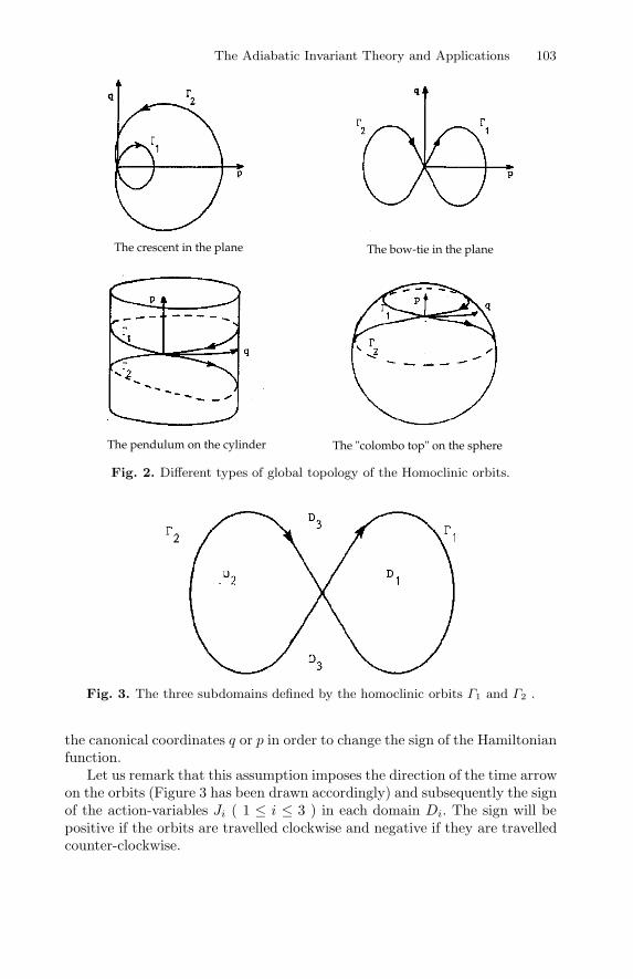
The Adiabatic Invariant Theory and Applications 103
The crescent in the plane The bow-tie in the plane
The pendulum on the cylinder The "colombo top" on the sphere
Fig. 2. Different types of global topology of the Homoclinic orbits.
Fig. 3. The three subdomains defined by the homoclinic orbits Γ1 and Γ2 .
the canonical coordinates q or p in order to change the sign of the Hamiltonianfunction.
Let us remark that this assumption imposes the direction of the time arrowon the orbits (Figure 3 has been drawn accordingly) and subsequently the signof the action-variables Ji ( 1 ≤ i ≤ 3 ) in each domain Di. The sign will bepositive if the orbits are travelled clockwise and negative if they are travelledcounter-clockwise.
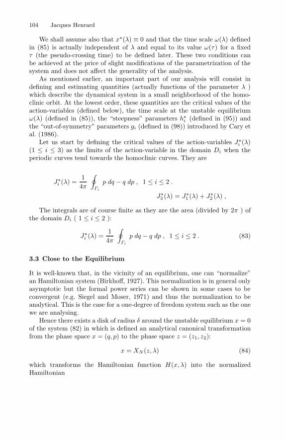
104 Jacques Henrard
We shall assume also that x(λ) ≡ 0 and that the time scale ω(λ) definedin (85) is actually independent of λ and equal to its value ω(τ) for a fixedτ (the pseudo-crossing time) to be defined later. These two conditions canbe achieved at the price of slight modifications of the parametrization of thesystem and does not affect the generality of the analysis.
As mentioned earlier, an important part of our analysis will consist indefining and estimating quantities (actually functions of the parameter λ )which describe the dynamical system in a small neighborhood of the homo-clinic orbit. At the lowest order, these quantities are the critical values of theaction-variables (defined below), the time scale at the unstable equilibriumω(λ) (defined in (85)), the “steepness” parameters hi (defined in (95)) andthe “out-of-symmetry” parameters gi (defined in (98)) introduced by Cary etal. (1986).
Let us start by defining the critical values of the action-variables Ji (λ)(1 ≤ i ≤ 3) as the limits of the action-variable in the domain Di when theperiodic curves tend towards the homoclinic curves. They are
Ji (λ) =14π
∮
Γi
p dq − q dp , 1 ≤ i ≤ 2 .
J3 (λ) = J1 (λ) + J2 (λ) ,
The integrals are of course finite as they are the area (divided by 2π ) ofthe domain Di ( 1 ≤ i ≤ 2 ):
Ji (λ) =14π
∮
Γi
p dq − q dp , 1 ≤ i ≤ 2 . (83)
3.3 Close to the Equilibrium
It is well-known that, in the vicinity of an equilibrium, one can “normalize”an Hamiltonian system (Birkhoff, 1927). This normalization is in general onlyasymptotic but the formal power series can be shown in some cases to beconvergent (e.g. Siegel and Moser, 1971) and thus the normalization to beanalytical. This is the case for a one-degree of freedom system such as the onewe are analysing.
Hence there exists a disk of radius δ around the unstable equilibrium x = 0of the system (82) in which is defined an analytical canonical transformationfrom the phase space x = (q, p) to the phase space z = (z1, z2):
x = XN (z, λ) (84)
which transforms the Hamiltonian function H(x, λ) into the normalizedHamiltonian
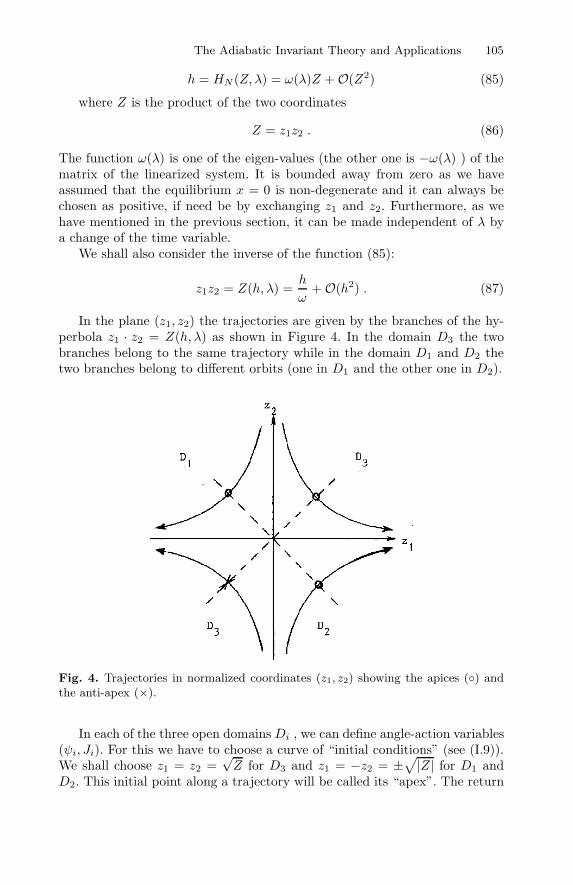
The Adiabatic Invariant Theory and Applications 105
h = HN (Z, λ) = ω(λ)Z +O(Z2) (85)
where Z is the product of the two coordinates
Z = z1z2 . (86)
The function ω(λ) is one of the eigen-values (the other one is −ω(λ) ) of thematrix of the linearized system. It is bounded away from zero as we haveassumed that the equilibrium x = 0 is non-degenerate and it can always bechosen as positive, if need be by exchanging z1 and z2. Furthermore, as wehave mentioned in the previous section, it can be made independent of λ bya change of the time variable.
We shall also consider the inverse of the function (85):
z1z2 = Z(h, λ) =h
ω+O(h2) . (87)
In the plane (z1, z2) the trajectories are given by the branches of the hy-perbola z1 · z2 = Z(h, λ) as shown in Figure 4. In the domain D3 the twobranches belong to the same trajectory while in the domain D1 and D2 thetwo branches belong to different orbits (one in D1 and the other one in D2).
Fig. 4. Trajectories in normalized coordinates (z1, z2) showing the apices () andthe anti-apex (×).
In each of the three open domains Di , we can define angle-action variables(ψi, Ji). For this we have to choose a curve of “initial conditions” (see (I.9)).We shall choose z1 = z2 =
√Z for D3 and z1 = −z2 = ±
√
|Z| for D1 andD2. This initial point along a trajectory will be called its “apex”. The return
106 Jacques Henrard
point z1 = z2 = −√Z along a trajectory in D3 will be called the “anti-apex”.
Apex and anti-apex are called “vertex” by Cary et al. (1986).The normalizing transformation (84) is not uniquely defined although the
normalized Hamiltonian (85) is uniquely defined. This makes the definition ofthe apices coordinate-dependent. We shall come back on this later.
The transformation from the normalizing coordinates (z1, z2) to the angle-action variables (ψi, Ji) of each domain Di are easy to define. The generatingfunctions S′(z1, Ji, λ) is (see (24)):
S′i(z1, Ji, λ) =
∫ z1
±√
|Zi|
Ziz1dz1 +
12Zi = ±1
2Zi log
z21e
|Zi|(88)
where Zi is a yet unknown function of Ji and λ. Its definition depends uponthe global properties of the trajectory and it cannot be determined by theanalysis of this section which is purely local being confined to the disk of ra-dius δ around the origin. We shall determine this function or rather its inverseJi = Ji(Z, λ) in the next section.
Note that a “±” sign is inserted in (88) and in what follows, to indicate thatthe sign of the function should be ajusted (in an obvious way) in accordancewith the quadrangle of the plane (z1, z2) to which the domain Di belongs.
When we consider that λ = εt , the normalizing transformation (84) andthe transformation to action-angle variables are time-dependent. The remain-der function to be added to HN in order to produce the “new Hamiltonian” ofthe dynamical system is the sum of the remainder function of the normalizingtransformation RN (z, λ) and the remainder function of the transformation toaction-angle variables, R′
i(ψi, Ji, λ).The equilibrium x = 0 being sent on z = 0 , the normalizing transforma-
tion has no independent term and the remainder function RN has no linearterm
RN (z, λ) = O(||z||2) . (89)
On the other hand, we have for the second remainder function:
R′i(ψi, Ji, λ) =
∂S′
∂λ= ±1
2
(∂Zi∂λ
)
logz21
|Zi|=(∂Zi∂λ
)(∂Zi∂Ji
)−1
ψi .
Summing the two contributions and defining the function Ji = Ji(Z, λ) asthe inverse of the yet unknown function mentioned earlier, we have
Ri(ψi, Ji, λ) = −(∂Ji∂λ
)
ψi +RN (z, λ) . (90)
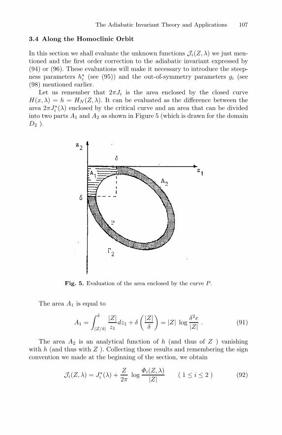
The Adiabatic Invariant Theory and Applications 107
3.4 Along the Homoclinic Orbit
In this section we shall evaluate the unknown functions Ji(Z, λ) we just men-tioned and the first order correction to the adiabatic invariant expressed by(94) or (96). These evaluations will make it necessary to introduce the steep-ness parameters hi (see (95)) and the out-of-symmetry parameters gi (see(98) mentioned earlier.
Let us remember that 2πJi is the area enclosed by the closed curveH(x, λ) = h = HN (Z, λ). It can be evaluated as the difference between thearea 2πJi (λ) enclosed by the critical curve and an area that can be dividedinto two parts A1 and A2 as shown in Figure 5 (which is drawn for the domainD2 ).
Fig. 5. Evaluation of the area enclosed by the curve P .
The area A1 is equal to
A1 =∫ δ
|Z/δ|
|Z|z1dz1 + δ
(|Z|δ
)
= |Z| logδ2e
|Z| . (91)
The area A2 is an analytical function of h (and thus of Z ) vanishingwith h (and thus with Z ). Collecting those results and remembering the signconvention we made at the beginning of the section, we obtain
Ji(Z, λ) = Ji (λ) +Z
2πlog
Φi(Z, λ)|Z| ( 1 ≤ i ≤ 2 ) (92)
108 Jacques Henrard
where the functions Φi(Z, λ) = δ2e exp(A2/|Z|) are analytical functions. Thesetwo functions are invariants of the dynamical system and, together with thefunction Z(h, λ) , they characterize it completely. These are the functions weintroduced in the previous section. The functional dependences of Ji withrespect to h:
Ji(h, λ) = Ji(Z(h, λ), λ) (1 ≤ i ≤ 2) (93)
will also be most useful. Their approximations close to the homoclinic orbitsare given by
Ji(h, λ) = Ji (λ) +h
2πωlog
ehi|h| +O(h2 log |h−1|) , (94)
The parameters
hi (λ) =ω(λ)e
Φi(0, λ) ( 1 ≤ i ≤ 2 ) (95)
are the “steepness parameters” mentionned earlier. They measure the ratesat which Ji approach Ji when h goes to zero. As such they will enter in manyof our estimates.
Formula (92) is valid for the two domains D1 and D2. In order to evaluatethe area enclosed by a trajectory in the domain D3 , we have to add twice thearea A1 plus the two areas of the type A2 corresponding to each lobe alongΓ1 and Γ2. We find
J3(Z, λ) = J3 (λ) +Z
πlog
Φ3(Z, λ)|Z|
with
Φ3(Z, λ) = [Φ1(Z, λ) Φ2(Z, λ)]1/2 , J3 (λ) = J1 (λ) + J2 (λ) .
Hence J3 is approximated by
J3(h, λ) = J3 (λ) +h
πωlog
eh3|h| +O(h2 log |h−1|) , (96)
withh3(λ) = [h1 h
2]
1/2 . (97)
We turn now to the evaluation of the first order corrections to the adiabaticinvariants for small (but not too small) values of h. From (52), we have
Ji = Ji + ε (∂Ji∂h
) R(ψi, Ji, λ)− < R(ψi, Ji, λ) >+O(ε2h−1 log2 |h−1|) .
In estimating the error term, we made use of (52) but also of (94) in order toestimate the derivatives of h with respect to Ji.
The Adiabatic Invariant Theory and Applications 109
We shall evaluate the adiabatic invariant Ji at the apex ( ψi = 0 ). From(90) we have that
Ri(0, Ji, λ) = RN (±√
|Z|,±√
|Z|) = O(|Z|) = O(h) .
It remains to evaluate the mean value of the remainder functions. Aftersome computation (see (Henrard 1993) for details) we find
< Ri > =(∂Ji∂h
)−1
−gi(λ) +O(h log |h−1|)
1 ≤ i ≤ 2 ,
< R3 > =(∂J3
∂h
)−1
−g3(λ) + π∆12 +O(h log |h−1|)
,
with∆12 =
∂J1
∂λ
∂J2
∂h− ∂J2
∂λ
∂J1
∂h
andg3(λ) = g1(λ) + g2(λ) . (98)
The functions gi(λ) , which are important because they measure the firstorder corrections to the adiabatic invariants (see below), vanish when thefunctions Ri ( 1 ≤ i ≤ 2 ) are odd in ψ. This is the case when the dynamicalsystem possesses the right type of symmetry and when the apices are chosenaccordingly. This is why we have called these functions the “out-of-symmetry”parameters. Most of the simple dynamical systems have the right type ofsymmetry and the corresponding functions gi(λ) vanish. For more generalsystems, the functions can be evaluated numerically, for instance, by meansof the numerical integration of the variational equations.
Gathering these results, we find that the adiabatic invariants in each ofthe three domains Di are given by
Ji = Ji + εgi +O(εh log |h−1|, ε2h−1 log2 |h−1|) 1 ≤ i ≤ 2 , (99)J3 = J3 + εg3 − π∆12+O(εh log |h−1|, ε2h−1 log2 |h−1|) (100)
where the Ji ( 1 ≤ i ≤ 2 ) are evaluated at the apices.
3.5 Traverse from Apex to Apex
We shall now be concerned with solutions of the non-autonomous systemdescribed by the Hamiltonian function:
H(x, εt) = h(t) . (101)
As we have seen in Section 3.3, this system is equivalent in a disk of radiusδ around the origin, to the system described by
H ′(z, εt) = HN (Z, εt) + ε RN (z1, z2, εt) (102)
in the normalizing coordinates (z1, z2).
110 Jacques Henrard
We shall be concerned more specifically with a “traverse” from apex toapex (or from apex to anti-apex) close to one of the homoclinic orbits Γi.
Let us assume that at time t0 , a trajectory of (101) is at an apex (oranti-apex) with h = h0, λ = λ0 , z2
1 = z22 = ζ2
0 = |Z(h0, λ0)| , and thatthe following apex (or anti-apex) corresponds to t = t1 , h = h1 , λ = λ1 ,z21 = z2
2 = ζ21 = |Z(h1, λ1)|.
We plan to evaluate the difference in “energy” and in time between thosetwo consecutive apices:
∆h = h1 − h0 , ∆λ = λ1 − λ0 = ε ∆T = ε (t1 − t0) . (103)
In order to obtain these estimates, we compare the solution of the non-autonomous system (101) (or (102)) which passes through an apex at timeλj/ε with the energy hj :
x(t, hj , λj) or z(t, hj , λj) (1 ≤ j ≤ 2 ) . (104)
with the solution of the autonomous system described byH(x, λj) or HN (Z, λj) which we denote
x(t, hj , λj) or z(t, hj , λj) = (ζj expΩjt , ζj exp−Ωjt) (105)
where Ωj = Ω(ζ2j , λj) , the function Ω being the derivative ∂HN/∂Z.
The comparison is quite delicate if one wishes to reach very small valuesof h0 (of the order of exp−1/ε ) which implies very long periods of time (ofthe order of 1/ε ).
The main step (developed in detail in Henrard 1993) is to compare, inthe disk of radius δ around the origin, the solution z(t, hj, λj) of the non-autonomous system with the solution
u = (ζj expµj(t), ζj exp−µj(t)) , µj =∫ t
tj
Ω(ζ2j , εt) dt , (106)
of the intermediary system described by HN (Z, εt).We find the estimate
||z − u|| ≤ c6ε for c7 exp− 1c1ε ≤ hj ≤ c5 (107)
where c1, c5, c6, c7 are constants independent of ε.It is for the comparison of u and z that the assumption we have made
that ω is independent of λ is useful. Indeed this assumption makes the esti-mate, in the disk of radius δ around the origin:
|µj −Ωjt| ≤ c8εhj log |h−1j | (108)
The Adiabatic Invariant Theory and Applications 111
sharper than the corresponding estimate (|µj −Ωjt| ≤ c8ε log |h−1j |) to which
one would be led if ω , the leading term in Ω , were indeed a function of time.The estimate (108) leads to a total estimate
||z − z|| ≤ c9ε (109)
in the disk of radius δ around the unstable equilibrium.The value of ∆T , the time spent from apex (h0, λ0) to the next one
(h1, λ1) is then estimated as follows. Let
∆T = T ε0 + T ε1 + T εδ (110)
where T ε0 (h0, λ0) and T ε1 (h1, λ1) are the values of the time spent in the diskof radius δ in the neighborhood of the two apices and T εδ the value of thetime spent outside this disk. The superscript ε is there to recall that we areconsidering the non-autonomous system with λ = εt.
From lengthty computations (see Henrard 1993), we get an estimate for∆T as a mean value of the periods of two trajectories of the autonomoussystem, the initial conditions of which correspond to the value of h and λ atthe apices
∆T =12T (h0, λ0) + T (h1, λ1)+O(ε log h−1
m )
= π(∂J∂h
(h0, λ0) + (∂J
∂h)(h1, λ1)+O(ε log h−1
m ) , (111)
where hm is the minimum value of h0 and h1. We now proceed by estimating∆h:
∆h = h1 − h0 = ε
∫ t1
t0
∂H
∂λ(x, εt) dt . (112)
The integral can be split into two parts: One starting from t0 on an intervalof T (h0, λ0)/2 and the other one on an interval T (h1, λ1)/2 ending at t1. Eachof these integrals is then compared with the corresponding integrals withx(t, hi, λi) substituted to x and λi substituted to εt . We obtain eventually(see (Henrard, 1993) for details)
∆h = ε
∫ T (hj ,λj)
0
∂H
∂λ(xj , λj) dt+O(ε2 log h−1
m ) . (113)
where the subscript j may be taken indifferently as 0 or 1.It remains to compute the integral in the right-hand member of (113).
112 Jacques Henrard
From (43) we compute:
R(2π)−R(0) =(∂K
∂J
)−1 ∫ 2π
0
[∂H
∂p
∂P ∗
∂λ+∂H
∂q
∂Q∗
∂λ
]
dψ
=(∂K
∂J
)−1 ∫ 2π
0
[d
dλH(Q∗, P ∗, λ)− ∂H
∂λ
]
dψ
=(∂K
∂J
)−1 ∫ 2π
0
[∂K
∂λ− ∂H
∂λ
]
dψ ,
because H(Q∗, P ∗, λ) = K(J, λ). As the remainder function is periodic, theabove integral is zero. We conclude that
∫ ∞
0
∂H
∂λ(x∗j , λj) dt =
(∂K
∂J
)−1 ∫ 2π
0
∂K
∂λdψ = 2π
(∂K
∂J
)−1∂K
∂λ.
Eventually we obtain
∆h = −2πε(∂J
∂λ
)
(hj , λj) +O(ε2 log |h−1m |) . (114)
The last equality is obtained by differentiating K(J(h, λ), λ) = h with respectto λ.
The approximations (111) and (114) define mappings from (h0, λ0) to(h1, λ1) , from apex to apex in each of the domains Di. These mappingsreproduce (approximately) the behaviour of the non-autonomous dynamicalsystem in the vicinity of the homoclinic orbit. They are Poincare’s mappingswith the apices defining the surfaces of section.
In what follows we shall use only an approximation of this mapping whichis easier to handle. It is obtained by substituting the approximations (94) forthe functions Ji
∆λi =ε
2ω
loghi|h0|
+ loghi|h1|
+O(ε2 log |h−1m |, εhM log h−1
M ) ;
∆hi = −2πε(∂Ji∂λ
)
+O(ε2 log |h−1m |, εhM log h−1
M ) . (115)
The subscripts (i) in ∆hi , ∆λi have been inserted to recall that themapping is different in each of the domains Di. The functions ω(λ) , hi (λ)and Ji (λ) are evaluated at λ = λ0. We recall also that hm (resp. hM ) standsfor the minimum (resp. maximum) of the absolute values of h0 and h1.
Formulae (115) are not meaningful if ε log |h−1m | is not small. We thus make
the assumptionhm ≥ εη >> exp−ε−1 . (116)
The Adiabatic Invariant Theory and Applications 113
Later, we shall be led to the choice
η =1ε
exp−ε−1/3 (117)
in order to minimize the error terms on the final results.
3.6 Probability of Capture
We are now in a position where we can analyse the transition from one domainto another one. We shall investigate in this section the basic question: wheredoes the trajectory go when, from inside the domain Di (which is shrinking),it is pushed towards the critical curve ? Does it stay indefinitely close to thecritical curve ? Does it end up eventually well inside one of the other domainsDj where the adiabatic invariant can again inform us about its ultimate fate,and which one of the other domains ?
We shall show that, except for a set of initial conditions, the measure ofwhich is exponentially small with ε , the trajectory does end up in one of theother two domains after a time such that the parameter λ has not changedsignificantly.
In some cases we shall be able to say which one of the other domains isvisited. In other cases, it depends very sensitively upon the initial conditions.So sensitively that the accuracy on the initial conditions needed to decidewhich one it is, is not physically meaningful and, as a consequence, we shallresort to a probabilistic argument.
Let us first investigate the case where the trajectory is initially in domainD3 and approaches the critical curve close enough so that the formula (115)becomes meaningful. As we are approaching the critical curve and not goingaway from it, ∆h3 , the increment of h (see (59)), is negative and, at eachturn, from apex to apex, the value of h decreases by an amount proportionalto ε (we assume of course that the ∂Ji /∂λ are bounded away from zero).Eventually, h takes on a value h0 such that
0 < h0 ≤ −∆h3 . (118)
This is the last time the trajectory goes through the apex in domain D3.We shall call it the main apex. As we use the approximation (115), we haveto exclude from our consideration, initial conditions such that h0 comes closerto one of its limiting values ( 0 and −∆h3 ) than εη (see 116).
This is part of the set of initial conditions we were mentioning earlier andfor which our analysis fails. The corresponding trajectories could stay for avery long time, possibly forever, close to the “unstable equilibrium”. Notethat the “unstable equilibrium” is an equilibrium of the “frozen” system withλ constant. In the system we are analysing, with λ = εt, the equilibrium maybe replaced by a very complicated invariant set.
114 Jacques Henrard
Let us assume now that the two domains Di ( 1 ≤ i ≤ 2 ) increasein size. It means that ∆h1 and ∆h2 (see (115)) are also negative and that∆h3 = ∆h1 + ∆h2 is larger in absolute value than either of them. If h0
happens to be in the interval
εη ≤ h0 ≤ −∆h1 − εη , (119)
the first traverse along Γ1 after that will bring the trajectory inside the domainD1 with a negative value of h. From there-on, the trajectory will loose energyat the rate of ∆h1 for each turn in D1 and will end up well inside this domain.
On the other hand, if h0 is in the interval
−∆h1 + εη < h0 < −∆h3 − εη , (120)
the trajectory will arrive at the anti-apex in domain D3 with a value of theenergy equal to h′0 = h0 +∆h1 , with
εη < h′0 < −∆h2 − εη . (121)
The traverse along Γ2 after this will bring the trajectory inside D2 andfrom there-on it will go deeper and deeper in D2.
If we do not know the exact value of h0 but assume that the distribu-tion of possible values is uniform on the interval of definition (118) (we shallcome back on this assumption later), the probability of the trajectory endingup in Di is proportional to the length of the interval (119) or (121). As aconsequence, we have
Pi =∆hi∆h3
=∂Ji∂λ
/∂J3∂λ
+O(ε log(εη)−1) (122)
where Pi is the probability of the trajectory ending up in domain Di. Withthe assumption (118), the error term is ε2/3.
If, on the other hand, the two domains Di ( 1 ≤ i ≤ 2 ) do not increasein size but only one of them does, say D1 , the trajectory will certainly endup in that domain. Indeed only ∆h1 is negative and the trajectory can onlyleave D3 along Γ1 and enters then D1. Once it has entered it, it will remainin it, decreasing its energy by ∆h1 at each traverse.
Let us investigate now the case where the trajectory is initially in one ofthe two domains Di ( 1 ≤ i ≤ 2 ). Let us choose D2 to simplify the notations.
The value of ∆h2 is then positive (as we are approaching the critical curve)and we shall eventually enter the domain D3 (except possibly for an exponen-tially small set of initial conditions). At the first apex in Domain D3, whichwe shall call the main apex, the energy is h0 with
εη < h0 < ∆h2 − εη (123)
as we have crossed h = 0 in the last traverse along Γ2 just before this apex.
The Adiabatic Invariant Theory and Applications 115
Again we have to consider two cases according to the sign of ∆h1. If it ispositive, the energy will increase at each successive traverse and the trajectorywill end up in D3.
If ∆h1 is negative and if h0 happens to fall in the interval
εη ≤ h0 ≤ −∆h1 − εη , (124)
the trajectory will enter the domain D1 on its first traverse along Γ1 and willremain there loosing energy at each successive traverse in D1.
If h0 does not belong to the interval (124), it means that it belongs to
−∆h1 + εη ≤ h0 ≤ ∆h2 − εη (125)
and that −∆h1 < ∆h2 or that ∆h3 = ∆h2 +∆h1 > 0. Hence the trajectorydoes not enter D1 on its first traverse along Γ1 and increases its energy by∆h3 on the total trip from apex to apex. This will be true for the successivetrips from apex to apex until formula (115) is no longer valid and we are deepenough in domain D3.
Again if we do not know the exact value of h0 but assign a uniform dis-tribution of probability on its value in the domain of definition (123), theprobability Pi of the trajectory ending up in Di (i = 1 or 3) is proportionalto the length of the intervals (124) or (125):
P1 = −∂J1
∂λ/∂J2∂λ
+O(ε log(εη)−1) ,
P3 =∂J3∂λ
/∂J2∂λ
+O(ε log(εη)−1) .
The various cases we have analysed may be summarized in a unique for-mula. We may consider a jump from domain Di to domain Dj (1 ≤ i, j ≤ 3)if the trajectories are leaving Di , i.e.
leaving Di : sgn(hi) ·(∂Ji∂λ
)
> 0 .
In that case, the probability of the jump from Di to Dj is given by:
Pr(i, j) = −sgn(hihj)∂Jj∂λ
/∂Ji∂λ
+O(ε log(εη)−1) , (126)
where sgn(hi) is the sign of h in the domain Di. Written in this way, Formulae(71) and (72) are independent of the assumption on the sign of h made inSection 3.2.
Of course, formula (126) should be understood with the following conven-tion. If the right-hand member is negative, the probability is actually zero andif the right-hand member is larger than one, the probability is actually one.

116 Jacques Henrard
We shall call the function Pr(i, j) the probability function. It is equal to theprobability of transition when its value lies between zero and one.
We ought to come back now on the assumption that h0 , the value of theHamiltonian at the main apex, is a random variable uniformly distributed onits interval of definition (see (118) or (123)).
When the probabilistic argument is introduced simply by our lack of knowl-edge about the precise initial conditions (or for that matter the precise mod-elization of the dynamical system) of a unique “test particle” as it happensin most problems of capture into resonance in Celestial Mechanics, then theassumption is as good as another one. On the other hand, if we are thinkingin terms of distribution of many test particles in a dynamical system as it isnatural in problems involving charged particles in a plasma, then it becomesimportant to relate the distribution on the values of h0 (at the main apex)with the distribution of initial conditions far from the transition. Neishtadt(1975) found that it is a simple consequence of Liouville’s Theorem.
We shall paraphrase Neishtadt’s argument by using Poincare-Cartan In-tegral Invariant.
Let us take two small sets of points Pi ( 1 ≤ i ≤ 2 ) in the extended phasespace (q, p, t). We take them at the main apex, centered respectively arounda value h0(i) of h0:
Pi : (q, p, t) such that
z1 = z2(apex) ,h0 ∈ [h0(i)− δh, h0(i) + δh] ,t ∈ [t0 − δt, t0 + δt] .
(127)
The values of the Integral Invariant for these sets of points are then∫ ∫
Pi
dq dp− dH dt = −∫ ∫
Pi
dH dt = −4δh · δt . (128)
Let us define Qi ( 1 ≤ i ≤ 2 ) as the sets of points in phase space translatedfrom Pi along the trajectories back to a time t = τ when they are far awayfrom the transition. As the integrals in (74) remain invariant, we have
∫ ∫
Qi
dq dp− dH dt =∫ ∫
Qi
dq dp = −4δh · δt .
The areas of the two sets of initial conditions Qi are then equal. Henceif the distribution of test particles in the phase-space far from transition isuniform, so is the distribution of values of h0 for test particles crossing theapex per unit of time.
We have assumed in the argument above a uniform distribution of testparticles in the full phase-space far from transition because it is the simplestassumption. Actually the set of points Qi can be shown to be very narrowstrips along the guiding trajectories far from transition (see Escande, 1985),and thus it is enough to assume that the distribution of test particles is uniformin ψ.
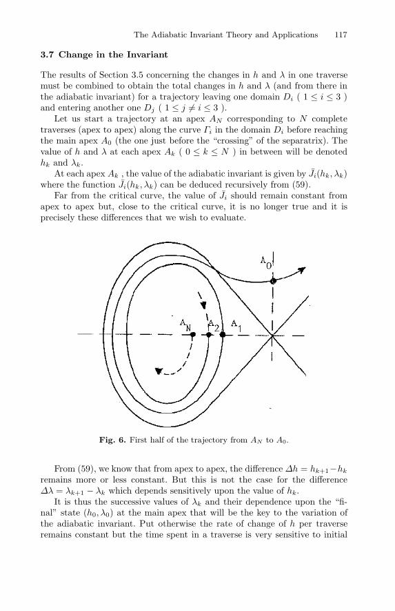
The Adiabatic Invariant Theory and Applications 117
3.7 Change in the Invariant
The results of Section 3.5 concerning the changes in h and λ in one traversemust be combined to obtain the total changes in h and λ (and from there inthe adiabatic invariant) for a trajectory leaving one domain Di ( 1 ≤ i ≤ 3 )and entering another one Dj ( 1 ≤ j = i ≤ 3 ).
Let us start a trajectory at an apex AN corresponding to N completetraverses (apex to apex) along the curve Γi in the domain Di before reachingthe main apex A0 (the one just before the “crossing” of the separatrix). Thevalue of h and λ at each apex Ak ( 0 ≤ k ≤ N ) in between will be denotedhk and λk.
At each apex Ak , the value of the adiabatic invariant is given by Ji(hk, λk)where the function Ji(hk, λk) can be deduced recursively from (59).
Far from the critical curve, the value of Ji should remain constant fromapex to apex but, close to the critical curve, it is no longer true and it isprecisely these differences that we wish to evaluate.
Fig. 6. First half of the trajectory from AN to A0.
From (59), we know that from apex to apex, the difference ∆h = hk+1−hkremains more or less constant. But this is not the case for the difference∆λ = λk+1 − λk which depends sensitively upon the value of hk.
It is thus the successive values of λk and their dependence upon the “fi-nal” state (h0, λ0) at the main apex that will be the key to the variation ofthe adiabatic invariant. Put otherwise the rate of change of h per traverseremains constant but the time spent in a traverse is very sensitive to initial
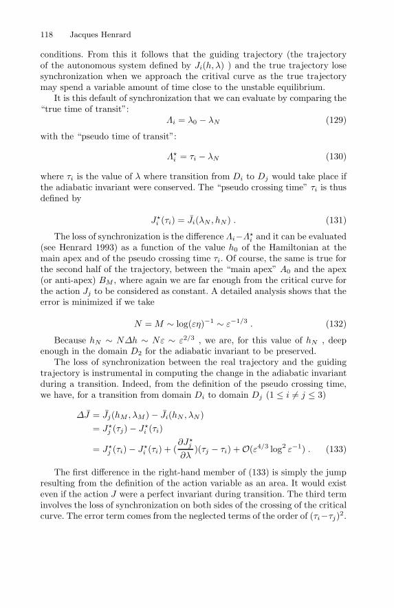
118 Jacques Henrard
conditions. From this it follows that the guiding trajectory (the trajectoryof the autonomous system defined by Ji(h, λ) ) and the true trajectory losesynchronization when we approach the critival curve as the true trajectorymay spend a variable amount of time close to the unstable equilibrium.
It is this default of synchronization that we can evaluate by comparing the“true time of transit”:
Λi = λ0 − λN (129)
with the “pseudo time of transit”:
Λi = τi − λN (130)
where τi is the value of λ where transition from Di to Dj would take place ifthe adiabatic invariant were conserved. The “pseudo crossing time” τi is thusdefined by
Ji (τi) = Ji(λN , hN ) . (131)
The loss of synchronization is the difference Λi−Λi and it can be evaluated(see Henrard 1993) as a function of the value h0 of the Hamiltonian at themain apex and of the pseudo crossing time τi. Of course, the same is true forthe second half of the trajectory, between the “main apex” A0 and the apex(or anti-apex) BM , where again we are far enough from the critical curve forthe action Jj to be considered as constant. A detailed analysis shows that theerror is minimized if we take
N = M ∼ log(εη)−1 ∼ ε−1/3 . (132)
Because hN ∼ N∆h ∼ Nε ∼ ε2/3 , we are, for this value of hN , deepenough in the domain D2 for the adiabatic invariant to be preserved.
The loss of synchronization between the real trajectory and the guidingtrajectory is instrumental in computing the change in the adiabatic invariantduring a transition. Indeed, from the definition of the pseudo crossing time,we have, for a transition from domain Di to domain Dj (1 ≤ i = j ≤ 3)
∆J = Jj(hM , λM )− Ji(hN , λN )= Jj (τj)− Ji (τi)
= Jj (τi)− Ji (τi) + (∂Jj∂λ
)(τj − τi) +O(ε4/3 log2 ε−1) . (133)
The first difference in the right-hand member of (133) is simply the jumpresulting from the definition of the action variable as an area. It would existeven if the action J were a perfect invariant during transition. The third terminvolves the loss of synchronization on both sides of the crossing of the criticalcurve. The error term comes from the neglected terms of the order of (τi−τj)2.
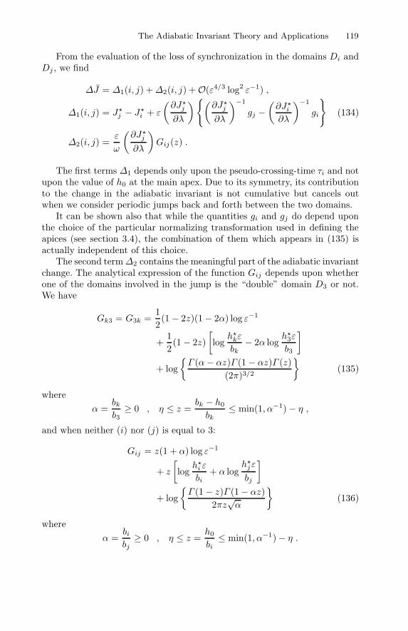
The Adiabatic Invariant Theory and Applications 119
From the evaluation of the loss of synchronization in the domains Di andDj , we find
∆J = ∆1(i, j) +∆2(i, j) +O(ε4/3 log2 ε−1) ,
∆1(i, j) = Jj − Ji + ε
(∂Jj∂λ
)(∂Jj∂λ
)−1
gj −(∂Ji∂λ
)−1
gi
(134)
∆2(i, j) =ε
ω
(∂Jj∂λ
)
Gij(z) .
The first terms ∆1 depends only upon the pseudo-crossing-time τi and notupon the value of h0 at the main apex. Due to its symmetry, its contributionto the change in the adiabatic invariant is not cumulative but cancels outwhen we consider periodic jumps back and forth between the two domains.
It can be shown also that while the quantities gi and gj do depend uponthe choice of the particular normalizing transformation used in defining theapices (see section 3.4), the combination of them which appears in (135) isactually independent of this choice.
The second term∆2 contains the meaningful part of the adiabatic invariantchange. The analytical expression of the function Gij depends upon whetherone of the domains involved in the jump is the “double” domain D3 or not.We have
Gk3 = G3k =12(1− 2z)(1− 2α) log ε−1
+12(1− 2z)
[
loghkε
bk− 2α log
h3ε
b3
]
+ logΓ (α− αz)Γ (1− αz)Γ (z)
(2π)3/2
(135)
whereα =
bkb3≥ 0 , η ≤ z =
bk − h0
bk≤ min(1, α−1)− η ,
and when neither (i) nor (j) is equal to 3:
Gij = z(1 + α) log ε−1
+ z
[
loghi ε
bi+ α log
hjε
bj
]
+ logΓ (1− z)Γ (1− αz)
2πz√α
(136)
whereα =
bibj≥ 0 , η ≤ z =
h0
bi≤ min(1, α−1)− η .
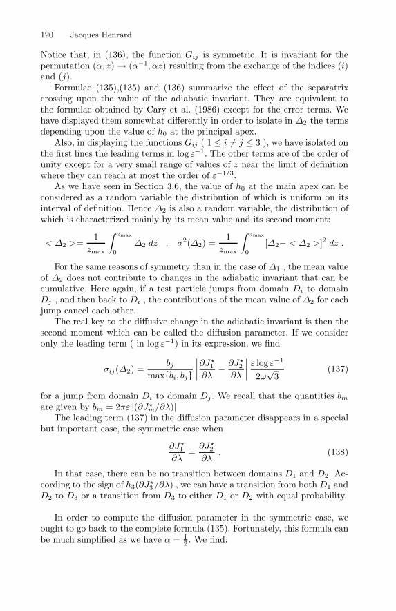
120 Jacques Henrard
Notice that, in (136), the function Gij is symmetric. It is invariant for thepermutation (α, z)→ (α−1, αz) resulting from the exchange of the indices (i)and (j).
Formulae (135),(135) and (136) summarize the effect of the separatrixcrossing upon the value of the adiabatic invariant. They are equivalent tothe formulae obtained by Cary et al. (1986) except for the error terms. Wehave displayed them somewhat differently in order to isolate in ∆2 the termsdepending upon the value of h0 at the principal apex.
Also, in displaying the functions Gij ( 1 ≤ i = j ≤ 3 ), we have isolated onthe first lines the leading terms in log ε−1. The other terms are of the order ofunity except for a very small range of values of z near the limit of definitionwhere they can reach at most the order of ε−1/3.
As we have seen in Section 3.6, the value of h0 at the main apex can beconsidered as a random variable the distribution of which is uniform on itsinterval of definition. Hence ∆2 is also a random variable, the distribution ofwhich is characterized mainly by its mean value and its second moment:
< ∆2 >=1
zmax
∫ zmax
0
∆2 dz , σ2(∆2) =1
zmax
∫ zmax
0
[∆2− < ∆2 >]2 dz .
For the same reasons of symmetry than in the case of ∆1 , the mean valueof ∆2 does not contribute to changes in the adiabatic invariant that can becumulative. Here again, if a test particle jumps from domain Di to domainDj , and then back to Di , the contributions of the mean value of ∆2 for eachjump cancel each other.
The real key to the diffusive change in the adiabatic invariant is then thesecond moment which can be called the diffusion parameter. If we consideronly the leading term ( in log ε−1) in its expression, we find
σij(∆2) =bj
maxbi, bj
∣∣∣∣
∂J1∂λ− ∂J2
∂λ
∣∣∣∣
ε log ε−1
2ω√
3(137)
for a jump from domain Di to domain Dj . We recall that the quantities bmare given by bm = 2πε |(∂Jm/∂λ)|
The leading term (137) in the diffusion parameter disappears in a specialbut important case, the symmetric case when
∂J1∂λ
=∂J2∂λ
. (138)
In that case, there can be no transition between domains D1 and D2. Ac-cording to the sign of h3(∂J3 /∂λ) , we can have a transition from both D1 andD2 to D3 or a transition from D3 to either D1 or D2 with equal probability.
In order to compute the diffusion parameter in the symmetric case, weought to go back to the complete formula (135). Fortunately, this formula canbe much simplified as we have α = 1
2 . We find:
The Adiabatic Invariant Theory and Applications 121
σij(∆2) =∣∣∣∣
∂Jj∂λ
∣∣∣∣
[
1 +1π2
log2 hi hj
h3h3
]1/2πε
2ω√
3. (139)
When the geometric symmetry (138) is accompanied by a time symmetrysuch that
h1 = h2 (140)
(which implies that h3 = h1 = h2 ), the second term of the square root in(101) disappears and we obtain:
σij(∆2) =∣∣∣∣
∂Jj∂λ
∣∣∣∣
πε
2ω√
3. (141)
This last formula is the one given by Timofeev (1978) in the case of thependulum with varying amplitude and by Cary et al. (1986) in the generalsymmetric case.
3.8 Applications
The Magnetic Bottle
As we mentionned in the second chapter, the model discussed there is, ofcourse, only approximative. Fluctuations in the magnetic field or electric fieldmay complicate the topology of the “frozen system” (corresponding to (75)with c = 0) by introduce a separatrix in the phase space. The adiabatic in-variance of the averaged G may then be in default at each crossing of theseparatrix.
This effect has been investigated for instance by Dobrott and Greene(1971) in the case of the stellator in which a weak but short periodicpoloidal magnetic field is superimposed on top of the main toroidal field(see also Kovrizhnykh, 1984) or by Aamodt (1971-1972) who considers short-wavelength fluctuations in the electric field due to collective modes in theplasma itself.
We shall discuss briefly this last application. Let us assume that superim-posed on the magnetic field (69), there is a short-wavelength electric field inthe direction perpendicular to the magnetic field and slightly modulated inthe direction of the magnetic field:
ϕ =m
eF (ε2x3) cos(kx1) . (142)
We introduce the “guiding center” coordinates as in (50) and a scaling ofthe third dimension:
y3 =1εz , Y3 = εZ (143)
122 Jacques Henrard
to obtain
K =12(1 + c)(Y 2
g + y2g) + F (εz) cos[
kYc1 + c
+kyg
(1 + c)1/2] +O(ε2) . (144)
As it can be seen in Figure 7, the motion (yg, Yg) can be severely distortedby the electric field corresponding to ϕ. This does not preclude the applicationof the adiabatic invariant theory and the definition of “mirror points”. Simply,the adiabatic invariant is no longer the (averaged) magnetic momentum G buta more complicated function and the mirror points are no longer given by (80).
YgYg
ygyg
c = oc = 1
Fig. 7. Motion of the particle around its gyrocenter for the Hamiltonian (63) withF = 2 , k = 1 , Yc = 0 and two particular values of c.
Of course the mirror points may be much different for a trapped orbit(inside the loops in Figure 7 than for un untrapped one (outside the loops).Also, we have to consider that the periodic jumps from one domain of thephase space of (yg, Yg) to another one generate a slow diffusion in the adiabaticinvariant which may be much more important than the one estimated byChirikov (see 81).
Resonance Sweeping in the Solar System
The orbital and spin parameters of many natural satellites in the Solar Sys-tem have been significantly affected by tidal dissipation and passage throughresonances. It is possible to understand the slow dynamical evolution of theseparameters in terms of a few “simple models” and the use of the adiabaticinvariant. Of course these simplified models do not always give an accuratequantitative answer to the problems at hand: too many physical parametersare poorly known and the mathematical approximations are sometime verycrude. But they can at least be used in order to define likely scenarii of evo-lution (or dismiss impossible or improbable scenarii) which can then, if needbe, improved either by refining the analytical model or by using numericalsimulations (which are often quite costly, since we are dealing with very slowevolutions).
Let us take as an example the passage through a second order resonanceof the planar planetary restricted three-body problem. The three bodies may
The Adiabatic Invariant Theory and Applications 123
be (Sun + Jupiter + Asteroid) or (Saturn + Mimas + particle in the ring) or(Uranus + Miranda + Umbriel).
The Hamiltonian of the restricted problem can be written:
H = − (1− µ)2
L2− µ
1
|r− r′| −r|r′
r′3
, (145)
where (1 − µ) and µ are the reduced masses of the primary and the sec-ondary, L =
√
(1− µ)a the first action variable of the two-body problem, athe semi-major axis of the test particle, r and r′ the position vector of the testparticle and of the secondary with respect to the primary. We are consideringhere that the Hamiltonian fonction is expressed implicitely in terms of theusual Delaunay’s modified elements where the quantities L, P are momentaconjugated to the angular variables λ, p, with
λ = mean longitude of particle , L =√
(1− µ)ap = −longitude of its pericenter , P = L
(
1−√
1− e2) (146)
where e is the eccentricity of the particle. The Hamiltonian is also a function ofthe time through its dependence upon the longitude of the secondary λ′ = n′t.In case of a 3/1 internal resonance between the unperturbed mean motion ofthe particle (n =
√
(1− µ)a3) we have
3n′ − n ≈ 0 . (147)
and it is usefull to introduce the Poincare’s resonance variables
σ = (3λ′ − λ+ 2p)/2 , S = P ,
ν = −(3λ′ − λ+ 2p′)/2 , N = 2L+ P − 2√
(1− µ)a∗ ,(148)
where a∗ is the “exact resonance” value: a∗ = a′[(1−µ)/9]1/3. After averagingthe Hamiltonian over the fast remaining angular variable λ′, the Hamiltonian,expanded in powers of
√S ≈ e and e′ reads
H = A(N − S)2 +BS + CS cos 2σ +De′2 cos 2ν
+ e′√S[E cos(σ + ν) + F cos(σ − ν)]
+ · · · . (149)
The coefficient A is of the order of unity, the coefficients C,D,E, F of theorder of µ (i.e ≈ 10−3 in the Sun-Jupiter problem and ≈ 10−5 in the Planet-Satellite problems. The coefficient B is also of the order of µ in the Sun-Jupiterproblem, but in the Planet-Satellite problems it should be corrected in orderto take into account the oblateness of the planet by a term of the order ofthe dynamical oblateness J2 which is of the order of 10−3 when the planet isUranus and 5 times larger when the planet is Saturn.
When B is not much larger than the trigonometric terms the unperturbedfrequencies of these terms are “small” for the same values of the momenta
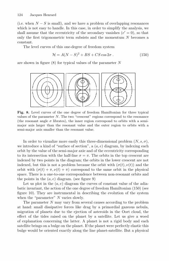
124 Jacques Henrard
(i.e. when N − S is small), and we have a problem of overlapping resonanceswhich is not easy to handle. In this case, in order to simplify the analysis, weshall assume that the eccentricity of the secondary vanishes (e′ = 0), so thatonly the first trigonometric term subsists and the momentum N becomes aconstant.
The level curves of this one-degree of freedom system
H = A(N − S)2 +BS + CS cos 2σ . (150)
are shown in figure (8) for typical values of the parameter N
Fig. 8. Level curves of the one degree of freedom Hamiltonian for three typicalvalues of the parameter N . The two “crescent” regions correspond to the resonance(the resonant angle σ librates), the inner region correspond to orbits with a semi-major axis larger than the resonant value and the outer region to orbits with asemi-major axis smaller than the resonant value.
In order to vizualize more easily this three-dimensional problem (N, s, σ),we introduce a kind of “surface of section”, a (a, e) diagram, by indexing eachorbit by the value of the semi-major axie and of the eccentricity correspondingto its intersection with the half-line σ = π. The orbits in the top crescent areindexed by two points in the diagram; the orbits in the lower crescent are notindexed, but this is not a problem because the orbit with (σ(t), ν(t)) and theorbit with (σ(t) + π, ν(t) + π) correspond to the same orbit in the physicalspace. There is a one-to-one correspondence between non-resonant orbits andthe points in the (a, e) diagram. (see figure 9)
Let us plot in the (a, e) diagram the curves of constant value of the adia-batic invariant, the action of the one degree of freedom Hamiltonian (150) (seefigure 10). They are instrumental in describing the evolution of the systemwhen the “parameter” N varies slowly.
The parameter N may vary from several causes according to the problemat hand: small dissipative forces like drag by a primordial gazeous nebula,migration of planets due to the ejection of asteroids in the Oort cloud, theeffect of the tides raised on the planet by a satellite. Let us give a woedof explanation concerning the latter. A planet is not a rigid body and eachsatellite brings on a bulge on the planet. If the planet were perfectly elastic thisbulge would be oriented exactly along the line planet-satellite. But a physical
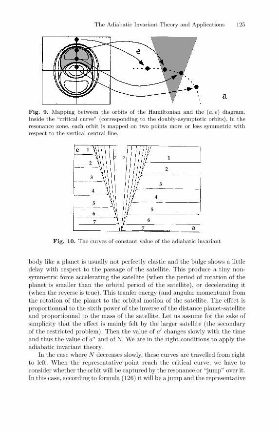
The Adiabatic Invariant Theory and Applications 125
Fig. 9. Mapping between the orbits of the Hamiltonian and the (a, e) diagram.Inside the “critical curve” (corresponding to the doubly-asymptotic orbits), in theresonance zone, each orbit is mapped on two points more or less symmetric withrespect to the vertical central line.
e
a
1
1
22
33
44
55
667
7
7 7
Fig. 10. The curves of constant value of the adiabatic invariant
body like a planet is usually not perfectly elastic and the bulge shows a littledelay with respect to the passage of the satellite. This produce a tiny non-symmetric force accelerating the satellite (when the period of rotation of theplanet is smaller than the orbital period of the satellite), or decelerating it(when the reverse is true). This tranfer energy (and angular momentum) fromthe rotation of the planet to the orbital motion of the satellite. The effect isproportionnal to the sixth power of the inverse of the distance planet-satelliteand proportionnal to the mass of the satellite. Let us assume for the sake ofsimplicity that the effect is mainly felt by the larger satellite (the secondaryof the restricted problem). Then the value of a′ changes slowly with the timeand thus the value of a∗ and of N. We are in the right conditions to apply theadiabatic invariant theory.
In the case where N decreases slowly, these curves are travelled from rightto left. When the representative point reach the critical curve, we have toconsider whether the orbit will be captured by the resonance or “jump” over it.In this case, according to formula (126) it will be a jump and the representative
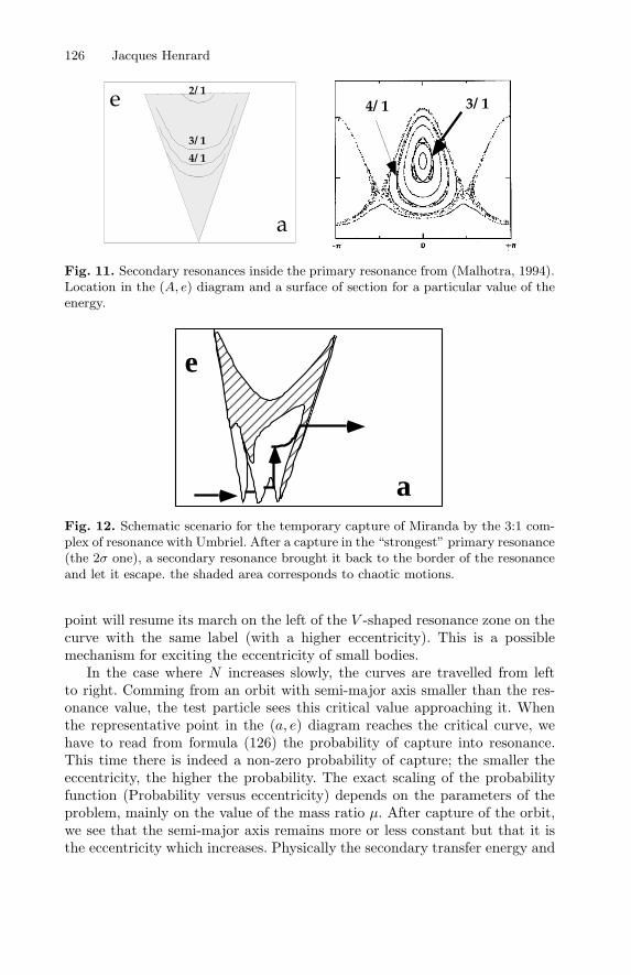
126 Jacques Henrard
3/ 14/ 1
a
e 2/ 1
3/ 1
4/ 1
Fig. 11. Secondary resonances inside the primary resonance from (Malhotra, 1994).Location in the (A, e) diagram and a surface of section for a particular value of theenergy.
a
e
Fig. 12. Schematic scenario for the temporary capture of Miranda by the 3:1 com-plex of resonance with Umbriel. After a capture in the “strongest” primary resonance(the 2σ one), a secondary resonance brought it back to the border of the resonanceand let it escape. the shaded area corresponds to chaotic motions.
point will resume its march on the left of the V -shaped resonance zone on thecurve with the same label (with a higher eccentricity). This is a possiblemechanism for exciting the eccentricity of small bodies.
In the case where N increases slowly, the curves are travelled from leftto right. Comming from an orbit with semi-major axis smaller than the res-onance value, the test particle sees this critical value approaching it. Whenthe representative point in the (a, e) diagram reaches the critical curve, wehave to read from formula (126) the probability of capture into resonance.This time there is indeed a non-zero probability of capture; the smaller theeccentricity, the higher the probability. The exact scaling of the probabilityfunction (Probability versus eccentricity) depends on the parameters of theproblem, mainly on the value of the mass ratio µ. After capture of the orbit,we see that the semi-major axis remains more or less constant but that it isthe eccentricity which increases. Physically the secondary transfer energy and
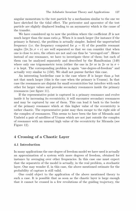
The Adiabatic Invariant Theory and Applications 127
angular momentum to the test particle by a mechanism similar to the one wehave sketched for the tidal effect. The pericenter and apocenter of the testparticle are slightly displaced leading to an asymmetry which is the cause ofthe transfer.
We have considered up to now the problem where the coefficient B is notmuch larger than the mass ratio µ. When it is much larger (for instance if theprimary is Saturn), the problem is actually simpler. Indeed the unperturbedfrequency (i.e. the frequency computed for µ = 0) of the possible resonantangles (2σ, 2ν, σ + ν) are well separated so that we can consider that whenone is close to zero, the others are not and can thus be “averaged out”. Henceinstead of one resonance, we have to investigate three of them; but each ofthem can be analyzed separately and described by the Hamiltonian (149)where only one trigonometric term (either the one in 2σ or in 2ν or in σ +ν is kept. The corresponding problem is again “one-degree-of-freedom” andactually very similar to (150). We shall not pursue further this case.
An interesting borderline case is the case where B is larger than µ butnot that much larger (this is the case when the primary is Uranus). In thatcase the resonances are disjoint for small eccentricities but interfere with eachother for larger values and provoke secondary resonances inside the primaryresonances (see figure 11).
If the representative point is captured in a primary resonance and evolveinside it by increasing its eccentricity, it will encounter secondary resonancesand may be captured by one of them. This can lead it back to the borderof the primary resonance which at this higher value of the eccentricity israther chaotic. The representative point may then escape to the right side ofthe complex of resonances. This seems to have been the fate of Miranda andUmbriel a pair of satellites of Uranus which are not just outside the complexof resonance with an unusual high value of the eccentricity for Miranda (seeFigure 12).
4 Crossing of a Chaotic Layer
4.1 Introduction
In many applications the one-degree of freedom model we have used is actuallyan approximation of a system with more degrees of freedom, obtained forinstance by averaging over other frequencies. In this case one must expectthat the separatrix of the model is actually, in the real problem, a stochasticlayer. One may wonder if, in this case, the above mentioned estimate for theprobability of capture is still valid.
One could object to the application of the above mentioned theory tosuch a case. It is possible that as soon as the chaotic layer is large enoughthat it cannot be crossed in a few revolutions of the guiding trajectory, the
128 Jacques Henrard
mechanism of capture is qualitatively different and thus the predictions of theabove mentioned theory have no relevance.
In this chapter, following (Henrard and Henrard, 1991 and Henrard andMorbidelli, 1992) we shall give indications that the situation is not as de-sesperate as that. Roughly speaking we shall show that there are reasons tobelieve that in the presence of a stochastic layer the probability of capture inthe growing domains (see the previous chapter) is still proportional to theirgrowing rates (see equation 172). The main difference will be that the “cap-ture” will no longer be instantaneous but will happen on a time scale inverselyproportional to the area of the stochastic layer (see equation 171). As a re-sult the change in the adiabatic invariant upon crossing the chaotic layer willhave a random component of the order of the area of the stochastic layer (seeequation 173).
4.2 The Frozen System
Let us consider the one-and-a-half degree-of-freedom Hamiltonian system de-pending upon a real parameter λ and defined by the Hamiltonian function:
H(q, p, t;λ) , (151)
T-periodic in the time t and defined on V ×T 1×I, where V is an oriented man-ifold parametrized by the canonical variables (q, p) and I is an open intervalof the real line.
The Poincare section of the system will be taken at t ≡ 0 (modulo T ) andthe Poincare map is the return map on the Poincare section: (q(0), p(0)) −→(q(T ), p(T )). The Poincare map is area-preserving. Indeed if C2 is the imageof a closed curve C1, we have by considering the Poincare linear integralinvariant [1]:
∫
C1
p dq =∫
C2
p dq . (152)
We shall assume that the dynamical system defined by the Poincare mapis a typical representative of a “close to integrable” and “close to a resonance”system. By this we mean the following. The Poincare section shows a finitenumber of simply connected domains Di where the Poincare map seems to beregular and one connected and bounded domain DS where the Poincare mapseems to be ergodic.
Generically we can expect that the Hamiltonian system we started withis not integrable and that if some invariant tori are present, they do not formopen domains of regular behaviour. But typically (see for instance Henon andHeile, 1964]), when the system is not too far away from an integrable one butclose to a resonance, we can expect to see in the Poincare section macroscopicregions which are almost completely filled by regular closed curves (trace ofinvariant tori upon the Poincare section) and a macroscopic region (aroundthe stable and unstable manifolds of the unstable periodic orbit generated by
The Adiabatic Invariant Theory and Applications 129
the resonance) which looks completely chaotic. We know of course that generi-cally the “regular” regions contain almost everywhere thin layers of stochasticbehaviour and that the stochastic region contains an infinite number of small“island”. The point is that the layers and the islands can be very small andthat we can hope to reach meaningful approximate answers about the systemby ignoring them.
In each regular domain Di of the Poincare section we define the action ofa regular closed curve C as the signed area:
A(C) =∫
C
p dq , (153)
where the sign of A(C) (the direction of the path integral) is chosen in sucha way that A(C) increases when the curve C approaches the boundary of theregular domain Di.
With such a definition we can characterize the regular domains Di by theirmaximum action:
Ai(λ) =∫
Γi
p dq , (154)
where Γi is the boundary of the regular domainDi with the stochastic domainDS . The sign of Ai(λ) is taken accordingly to the sign of the action in thedomain.
We shall assume in what follows that for λ ∈ I the number of regularregions is constant and furthermore that each of them grows (dAi/dλ > 0)or becomes smaller (dAi/dλ < 0) monotonically with λ. Let us call S+ theset of indices (i) such that dAi/dλ > 0 and S− the set of indices such thatdAi/dλ < 0 . We shall denote by A+(λ) (resp. A−(λ)) the sum of the actionsof the growing (resp. decreasing) regular domains:
A+(λ) =∑
i∈S+
Ai(λ) A−(λ) =∑
i∈S−Ai(λ) . (155)
4.3 The Slowly Varying System
We shall now assume that the parameter λ of the Hamiltonian function (151)is slowly changing with the time:
λ = εt . (156)
The Poincare section and the Poincare map are defined as previously. ThePoincare map is still area-preserving, but of course the dynamical systemdefined by the Poincare map will be different although we may expect thatit will not be very much different for time intervals small compared to ε−1.Our goal is of course to get information about the dynamical system for timeintervals of the order of ε−1.
130 Jacques Henrard
First let us show that in the regular domains the action as defined in (153)is adiabatically invariant. By this we mean that the changes in the action isof the order of ε for time intervals of the order of ε−1.
Indeed the image of a regular curve of Di remains adiabatically close toa regular curve of Di as long as this image remains in Di. To show thislet us remark that, in a regular domain, we can define approximate angle-action variables (ψ, J) such that for a fixed value of the parametrer λ, theHamiltonian (151) is transformed into
H = K(J ;λ) + ηP (ψ, J, t;λ) , (157)
where the “small parameter” η measures the non-integrability of the systemin the regular domain. We assume that it can be made as small as ε2.
If we consider now that λ = εt, the Hamiltonian of the system is no longergiven by (157) but by:
H ′ = K(J ; εt) + εR(ψ, J, t; εt) + ηP (ψ, J, t; εt) , (158)
where R is the remainder function of the time dependant canonical transfor-mation defining the action-angle variables.
A further averaging transformation brings the Hamiltonian (158) underthe form:
H ′ = K(J; εt) + εR(J ; εt) + ηP (ψ, J , t; εt) + ε2R(ψ, J , t; εt) , (159)
which shows that the averaged action J is an adiabatic invariant:
dJ
dt= O(ε2) . (160)
The action J itself, which differs from J by periodic terms of the order of ε isalso an adiabatic invariant.
Now if we consider at time t0 a closed regular curve C1 corresponding to agiven value of J , its image by an iterate of the return map will form a closedcurve C2. All the points on C2 will correspond within ε to the same value ofJ because J is an adiabatic invariant. Thus C2 is again a regular curve of thefrozen system and: ∫
C1
p dq =∫
C2
p dq . (161)
Hence the action as defined in (153) is adiabatically conserved.
4.4 Transition Between Domains
We wish to estimate statistically when and how a trajectory makes a transitionfrom one domain (regular or stochastic) of the frozen system to another one.We shall consider that the Poincare section is covered by particles with a
The Adiabatic Invariant Theory and Applications 131
density (q, p, n) where n is the number of the return map. The density isassumed to depend only upon the action in the regular domains and not onthe phase and to have a constant value S(n) in the stochastic domain.
Particles starting with an action A in one of the regular domain Di remainin this regular domain, with the same action, as long as A < Ai(εt) . But ifi ∈ S− (i.e. if the domain Di is one which is decreasing in area), the domainDi will loose particles to the stochastic domain at a rate of:
−idAidλ
ε , (162)
where i is the density of particles at the boundary of the domain Di.Indeed the particles contained between the regular curves of actionAi(ε(n+
1)T ) and Ai(εnT ) at time t = nT cannot remain in the regular domain att = (n+ 1)T .
On the other hand, the number of particles leaving the stochastic domainDS and entering the regular domain Dj (with j ∈ S+ ) at each iteration is
S(n)dAjdλ
ε , (163)
where S is the density of the stochastic domain at time t = nT . Indeedthe particles contained between the regular curves of action Aj(εnT ) andAj(ε(n + 1)T ) at time t = (n + 1)T cannot come from elsewhere than thestochastic domain. Their density (which is preserved because the map is area-preserving) was at time t = n equal to the density of the stochastic domain.
The above estimates are based upon the assumption that in the time εTa particle cannot jump directly from one regular domain to another one. It isassumed further that for most particles it takes many iterates of the Poincaremap to cross the stochastic domain. By “many” iterates we mean a numberlarge enough that the mixing character of the stochastic domain has the timeto uniformize the density of particles inside DS . It is difficult to translatequantitatively this assumption because we do not have a quantitative estimateof the mixing character ofDS . But certainly this assumption will be violated ifthe exchange of area between regular domains in one iteration of the mappingis of the order of the area of the stochastic domain. Hence we assume that:
dA+
dλεT AS ,
dA−
dλεT AS . (164)
Now let us follow the fate of a set of particles entering at time t = t0 thestochastic domain coming from one of the domain Di which is loosing area.Let us designate by k(t) the fraction of this set of particles which have leftthe stochastic domain at time t > t0. If t − t0 is large enough, the particlesremaining in the stochastic domain are spread uniformely and we can estimatethe number of them which are leaving the stochastic domain between t andt+ T , by using (163):
132 Jacques Henrard
k(t+ T )− k(t) =1− k(t)AS
dA+
dλεT . (165)
Indeed (1 − k(t))/AS(t) is the fractional density of the set of particleswe are considering and εTdA+/dλ measures the area lost by the stochasticdomain to the growing domains.
Converting (165) into a differential equation:
11− k
dk
dt=
ε
AS(t)dA+
dλ, (166)
and integrating, we find:
k(t) = 1− exp(−F+(t)) , (167)
with
F+(t) = ε
∫ t
t0
1AS(t)
dA+
dλdt . (168)
The fraction ki(t) of this set of particles which have entered the regulardomain Di (i ∈ S+) at time t is given by:
ki(t) = ε
∫ t
t0
1− k(t)AS(t)
dAidλ
dt . (169)
In the application described in the following sections we have that AS(t) =AS is a constant and so are the quantities:
B =dA+
dλC = −dA
−
dλBi =
dAidλ
(i ∈ S+) . (170)
In this case formulae (167) and (169) are easy to evaluate and we obtain:
k(t) = 1− exp[
−εB(t− t0)AS(t0)
]
, (171)
ki(t) =BiBk(t) . (172)
We conclude that the probability for one particle to enter a particulardomain Di is proportional to the growing rate Bi of this domain.
From (171) we can evaluate the distribution of the values of the action ofthe particle in the regular domain they have jumped into. The probability ofreaching the domain Di with a value of the action larger than Ai(0) +∆A isequal to:
Pr(Ai ≥ Ai(0) +∆A) = exp[
− BBi
∆A
AS
]
. (173)
In the limit AS → 0, these formulae agree with the formulae obtained byconsidering a separatrix crossing and not a chaotic layer crossing. In that case,as we recalled in the introduction, we have:
ki = Bi/B , Ai = Ai(0) . (174)
The Adiabatic Invariant Theory and Applications 133
4.5 The “MSySM”
As a test of the ideas developed in the previous sections we shall consideras “frozen system” the Modulated Symmetric Standard Map (in short theMSySM). Let us first describe the Symmetric Standard Map (in short theSySM):
(SySM)I(n+1) = I(n) −K sin
[
ϕ(n) + I(n)/2]
,
ϕ(n+1) = ϕ(n) +[
I(n+1) + I(n)]
/2 ,(175)
which can be interpreted as the application of a first order symplectic inte-grator, with a time step ε, to the integration of the pendulum. The parameterK = bε2 is a scaled value of the restoring force b of the pendulum and I = pε)is a scaled value of the momentum p.
We have shown in (Henrard and Morbidelli, 1992) how one can constructa formal power series which is a formal invariant for the sequence of pointsgenerated by the Symmetric Standard Map and we have shown how to com-pute it. Applying this technique we found that the action of the perturbedpendulum can be approximated by:
Jlib =8√K
π
µ1IE(α) − (µ1 + µ2)(1− α)IK(α)
, (176)
Jcirc =8√αK
π
µ1IE(β) + µ2(1− β)IK(β)
, (177)
where IK and IE are the usual elliptic function (see for instance Abramowiczand Stagun, 1968). The parameter α = β−1 is equal to (H + b)/2b and isequal to zero at the central stable equilibrium and one on the separatrix. Thecoefficient µ1 and µ2 are given as truncated series in ε by:
µ1 = 1 +K
72[1− 2α] (178)
− K2
5 400
[7916
+ 11α(1− α)]
+K3
7 938
[3 5932 560
− 1 205 α256
+19 α2
10(3− 2α)
]
− K4
17 010
[1 208 0871 228 800
− 1 553 α9 600
− 9 461 α2
3 200+
1 871 α3
600(2− α)
]
+K5
22 869
[181 980 143294 912 000
− 676 926 221 α442 368 000
− 13 699 639 α2
6 912 000
−17 166 013 α3
3 456 000+
2 953 α4
2 700(5− 2α)
]
134 Jacques Henrard
µ2 =αK
36+
11αK2
10 800[1− 2α] (179)
+αK3
7 938
[565256− 19 α
5(1− α)
]
+αK4
17 010
[89
4 800− 1 277 α
800+
1 871 α2
1 200(3 − 2α)
]
+αK5
76 230
[2 344 9011 638 400
− 3 226 493 α1 036 800
+3 595 391 α2
345 600− 2 953 α3
405(2 − α)
]
In order to obtain a model with a rather large and clean “stochastic layer”,we have imposed a slow modulation to the SySM by making K a function ofthe index n,
Kn = α∆2
[
1 + β cos(π(2n− 1)
N
)]
. (180)
This is the (normalized) second order symplectic integrator with time-step∆ (we shall reserve the symbol ε for a better use) for the modulated pendulumdescribed by the two degrees of freedom Hamiltonian,
H =12p2 + Λ+ α
[
1 + β cos2πλN
]
cos q , (181)
where λ is the time in disguise and Λ is its associated momentum. We call“modulated symmetric standard map” the N step map from t = λ = 0 tot = λ = N , i.e. the symplectic approximate integration of the pendulum overthe full period of the modulation.
For trajectories which do not cross the slowly moving separatrix of thependulum, the action J (see equations 176 and 177) is a second order (withrespect to 2π/N) adiabatic invariant (see for instance Arnold, 1963). Indeedthe first order correction is proportional to (∂H/∂λ) which in this case van-ishes at the time the mapping is evaluated (i.e. when λ = 0 mod 2π).
On the other hand, the trajectories which are forced to cross the slowlymoving separatrix are engulfed in a large and “clean” chaotic layer (see figure13). As shown by Elskens and Escande (1991), it is “clean” (i.e. has sharpboundaries and contains only very thin islands) because the “slowly pulsatingseparatrix sweep homoclinic tangles where islands must be small”. The extendof the chaotic layer can be easily approximated analytically. It corresponds(up to terms of order 2π/N) to the interval of values of the action which areassumed by the separatrix during its pulsation.
Inside the chaotic layer, the dynamics can be described (at least in a firstapproximation) as a diffusive process (Bruwhiler and Cary, 1989) on the actionJ together with a fast “phase mixing” on the angle variable (let us call it Ψ)conjugated to it. The diffusion coefficient of the Fokker-Planck equation forthe density P (J , t) of particles inside the chaotic layer
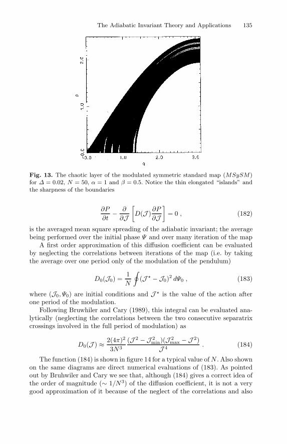
The Adiabatic Invariant Theory and Applications 135
Fig. 13. The chaotic layer of the modulated symmetric standard map (MSySM)for ∆ = 0.02, N = 50, α = 1 and β = 0.5. Notice the thin elongated “islands” andthe sharpness of the boundaries
∂P
∂t− ∂
∂J
[
D(J )∂P
∂J
]
= 0 , (182)
is the averaged mean square spreading of the adiabatic invariant; the averagebeing performed over the initial phase Ψ and over many iteration of the map
A first order approximation of this diffusion coefficient can be evaluatedby neglecting the correlations between iterations of the map (i.e. by takingthe average over one period only of the modulation of the pendulum)
D0(J0) =1N
∮
(J − J0)2 dΨ0 , (183)
where (J0, Ψ0) are initial conditions and J is the value of the action afterone period of the modulation.
Following Bruwhiler and Cary (1989), this integral can be evaluated ana-lytically (neglecting the correlations between the two consecutive separatrixcrossings involved in the full period of modulation) as
D0(J ) ≈ 2(4π)2
3N3
(J 2 − J 2min)(J 2
max − J 2)J 4
. (184)
The function (184) is shown in figure 14 for a typical value ofN . Also shownon the same diagrams are direct numerical evaluations of (183). As pointedout by Bruhwiler and Cary we see that, although (184) gives a correct idea ofthe order of magnitude (∼ 1/N3) of the diffusion coefficient, it is not a verygood approximation of it because of the neglect of the correlations and also
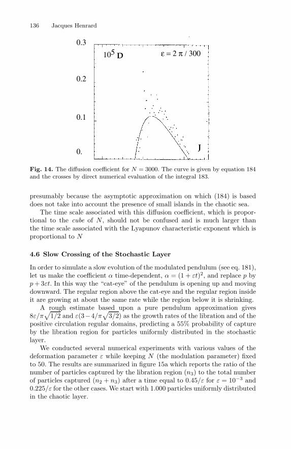
136 Jacques Henrard
105 D
J
0.1
0.2
0.3
0.
ε = 2 π / 300
Fig. 14. The diffusion coefficient for N = 3000. The curve is given by equation 184and the crosses by direct numerical evaluation of the integral 183.
presumably because the asymptotic approximation on which (184) is baseddoes not take into account the presence of small islands in the chaotic sea.
The time scale associated with this diffusion coefficient, which is propor-tional to the cube of N , should not be confused and is much larger thanthe time scale associated with the Lyapunov characteristic exponent which isproportional to N
4.6 Slow Crossing of the Stochastic Layer
In order to simulate a slow evolution of the modulated pendulum (see eq. 181),let us make the coefficient α time-dependent, α = (1 + εt)2, and replace p byp+ 3εt. In this way the “cat-eye” of the pendulum is opening up and movingdownward. The regular region above the cat-eye and the regular region insideit are growing at about the same rate while the region below it is shrinking.
A rough estimate based upon a pure pendulum approximation gives8ε/π
√
1/2 and ε(3−4/π√
3/2) as the growth rates of the libration and of thepositive circulation regular domains, predicting a 55% probability of captureby the libration region for particles uniformly distributed in the stochasticlayer.
We conducted several numerical experiments with various values of thedeformation parameter ε while keeping N (the modulation parameter) fixedto 50. The results are summarized in figure 15a which reports the ratio of thenumber of particles captured by the libration region (n3) to the total numberof particles captured (n2 + n3) after a time equal to 0.45/ε for ε = 10−3 and0.225/ε for the other cases. We start with 1.000 particles uniformly distributedin the chaotic layer.
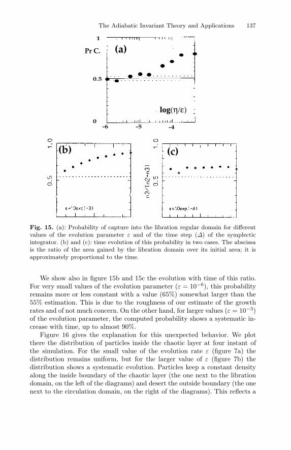
The Adiabatic Invariant Theory and Applications 137
-4-5-6
1
0.5
0
log(η/ε)
Pr C. (a)
(b) (c)
Fig. 15. (a): Probability of capture into the libration regular domain for differentvalues of the evolution parameter ε and of the time step (∆) of the symplecticintegrator. (b) and (c): time evolution of this probability in two cases. The abscissais the ratio of the area gained by the libration domain over its initial area; it isapproximately proportional to the time.
We show also in figure 15b and 15c the evolution with time of this ratio.For very small values of the evolution parameter (ε = 10−6), this probabilityremains more or less constant with a value (65%) somewhat larger than the55% estimation. This is due to the roughness of our estimate of the growthrates and of not much concern. On the other hand, for larger values (ε = 10−3)of the evolution parameter, the computed probability shows a systematic in-crease with time, up to almost 90%.
Figure 16 gives the explanation for this unexpected behavior. We plotthere the distribution of particles inside the chaotic layer at four instant ofthe simulation. For the small value of the evolution rate ε (figure 7a) thedistribution remains uniform, but for the larger value of ε (figure 7b) thedistribution shows a systematic evolution. Particles keep a constant densityalong the inside boundary of the chaotic layer (the one next to the librationdomain, on the left of the diagrams) and desert the outside boundary (the onenext to the circulation domain, on the right of the diagrams). This reflects a
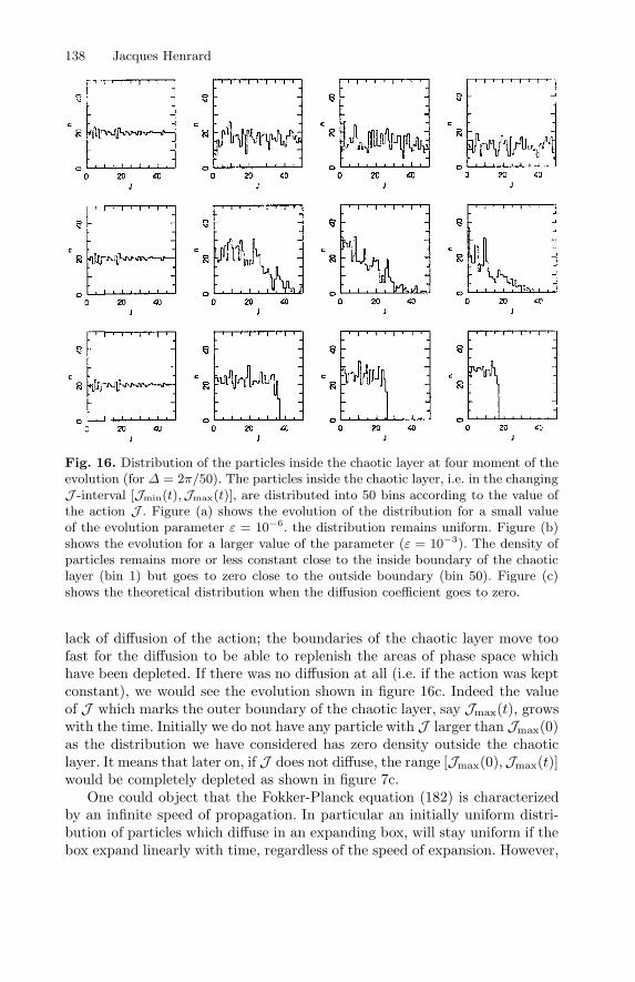
138 Jacques Henrard
Fig. 16. Distribution of the particles inside the chaotic layer at four moment of theevolution (for ∆ = 2π/50). The particles inside the chaotic layer, i.e. in the changingJ -interval [Jmin(t),Jmax(t)], are distributed into 50 bins according to the value ofthe action J . Figure (a) shows the evolution of the distribution for a small valueof the evolution parameter ε = 10−6. the distribution remains uniform. Figure (b)shows the evolution for a larger value of the parameter (ε = 10−3). The density ofparticles remains more or less constant close to the inside boundary of the chaoticlayer (bin 1) but goes to zero close to the outside boundary (bin 50). Figure (c)shows the theoretical distribution when the diffusion coefficient goes to zero.
lack of diffusion of the action; the boundaries of the chaotic layer move toofast for the diffusion to be able to replenish the areas of phase space whichhave been depleted. If there was no diffusion at all (i.e. if the action was keptconstant), we would see the evolution shown in figure 16c. Indeed the valueof J which marks the outer boundary of the chaotic layer, say Jmax(t), growswith the time. Initially we do not have any particle with J larger than Jmax(0)as the distribution we have considered has zero density outside the chaoticlayer. It means that later on, if J does not diffuse, the range [Jmax(0),Jmax(t)]would be completely depleted as shown in figure 7c.
One could object that the Fokker-Planck equation (182) is characterizedby an infinite speed of propagation. In particular an initially uniform distri-bution of particles which diffuse in an expanding box, will stay uniform if thebox expand linearly with time, regardless of the speed of expansion. However,
The Adiabatic Invariant Theory and Applications 139
one should not forget that the diffusion process we are dealing with here is adiscrete phenomenon with a basic time-scale given by the period of modula-tion N of the pendulum (i.e. the inverse of the Lyapunov exponent). In ourcase, the Fokker-Planck equation is valid only on time-scale much larger thanthis period of modulation. From this consideration one can get a rough andheuristic estimate of the maximum value of the evolution rate ε which allowsto keep an uniform density throughout the chaotic layer. After a time equal tothe modulation period the limit of the chaotic region Jmax(N) is changed bya quantity ∆J ≈ 8εN
√
α(1 + β/π which, in our case, amounts to 1.5 102ε.On the other hand, during the same period, the density of an interval of width
δJ ≈ η(Jmax − Jmin)√
DN/π , (185)
on the boundary will become uniform (with tolerance η) according to theFokker-Plank equation. If we impose ∆J δJ , we obtain (taking η = 10−1,D = 10−4, (Jmax − Jmin) = 1.3)
ε 3 10−5 . (186)
It does seems that the asymptotic estimate developed in the previous sec-tion for the probability of capture in regular domains for particles comingfrom the stochastic layer of a slowly evolving symplectic map is confirmed bythe numerical experiments on the modulated symmetric standard map. Butwe see that the asymptotic limit is reached only for rate of evolution muchsmaller than expected a priori. The reason for this is now identified. It is thefact that the value of the action diffuses on a time scale (proportional to thecube of the modulation coefficient N) much longer than the time scale of theLyapunov exponent (which is proportional to N).
References
1. Abramowitz, M. and Segun, I.A.: 1968, Handbook of Mathematical Functions,Dover Pub.
2. Alfven, H.: 1950, Cosmical Electrodynamics, Clarendon Press, Oxford.3. Andronov, A.A., Vitt, A.A. and Khaikin, S.E.: 1966, Theory of Oscillators,
Addison-Wesley, Reading, Mass.4. Arnold, V.I.: 1963, Small Denominators and Problems of Stability of Motion in
Classical and Celestial Mechanics, Russian Math. Survey, 18, 85-1915. Arnold, V.I., 1964, Small denominators and problems of stability of motion in
classical and celestial mechanics, Russian Math. Survey, 18, 85-191.6. Arnold, V.I.: 1978, Mathematical Methods of Classical Mechanics, Springer-
Verlag.7. Arnold, V.I.: 1985, Dynamical Systems III, Springer-Verlag8. Best, R.W.B.: 1968, On the motion of charged particles in a slightly damped
sinusoidal potential wave, Physica 40, 182-196.9. Cary, J.R., Escande, D.F. and Tennyson, J.L.: 1986, Adiabatic invariant change
due to separatrix crossing, Physical Review, A 34, 4256-4275.
140 Jacques Henrard
10. Chirikov, B.V.: 1979, A universal instability of many-dimensional oscillator sys-tems, Physics Reports, 52, 263-379.
11. Birkhoff, G.: 1927, Dynamical Systems, Am. Math. Soc. Coll. Pub. IX.12. Bruhwiler, D.L. and Cary, J.R.: 1989, Diffusion of Particles in a Slowly Modu-
lated Wave, Physica D, 40, 26513. Burns, T.J.: 1979, On the rotation of Mercury, Celestial Mechanics, 19, 297-313.14. Dobrott, D. and Greene, J.M.: 1971, Probability of trapping-state transitions in
a toroidal device, Phys. of Fluids, 14, 1525-1531.15. Dubrovin, B.A., Krichever, I.M. and Novikov, S.P.: 1985, Integrable Systems. I,
in Dynamical systems IV, Arnold and Novikov (eds), Springer-Verlag16. Elskens, Y. and Escande, D.F.: 1991, Slowly pulsating separatrices sweep ho-
moclinic tangles where island must be small: An extension of classical adiabatictheory, Nonlinearity, 4, 615-667
17. Escande, D.F.: 1985, Change of adiabatic invariant at separatrix crossing: Ap-plication to slow Hamiltonian chaos, in Advances in Nonlinear Dynamics andStochastic Processes, (R. Livi and A. Politi eds.), World Scientific Singapore,67-79.
18. Ferraz-Mello, S.: 1990, Averaging Hamiltonian Systems, in Modern Methods inCelestial Mechanics, Benest and Froeschle (eds), Editions Fronti‘eres
19. Freidberg, J.P.: 1982, Ideal magnetohydrodynamic theory of magnetic fusionsystems, Rev. of Modern Physics, 54, 801-902.
20. Goldreich, P.: 1965, An explanation of the frequent occurrence of commensurablemean motions in the Solar System, M.N.R.A.S., 130, 159-181.
21. Goldreich, P.: 1986, Final spin states of planets and satellites, Astron. J., 71,1-7.
22. Goldreich, P. and Peale, S.: 1966, Spin-orbit coupling in the Solar System, As-tron. J., 71, 425-437.
23. Hagihara, Y: 1970, Celestial Mechanics, Vol I, Mit Press, Cambridge24. Hannay, J.H.: 1986, Accuracy loss of action invariance in adiabatic change of a
one degree of freedom Hamiltonian, J. Phys. A, 19, 1067-1072.25. Henon, M. and Heiles, C.: 1964, The Applicability of the Third Integral of
Motion: some Numerical Experiments, Astron. Journal, 69, 73-7926. Henrard, J., 1982, Capture into resonance: An extension of the use of the adia-
batic invariants, Celestial Mechanics, 27, 3-22.27. Henrard, J.: 1990, Action-Angle Variables, in Modern Methods in Celestial Me-
chanics, Benest and Froeschle (eds), Editions Fronti‘eres28. Henrard, J.: 1993, The Adiabatic Invariant in Classical Mechanics, in Dynamics
Reported, Jones, Kirchgraber and Walther (eds), 2 new series, 117–23529. Henrard, J. and Henrard, M.: 1991, Slow Crossing of a Stochastic Layer, Physica
D, 54, 135-14630. Henrard, J. and Morbidelli, A.: 1993, Slow Crossing of a Stochastic Layer, Phys-
ica D, 68, 187-20031. Kovrizhnykh, L.M.:1984, Progress in stellarator theory, Plasma Phys., 26, 195-
207.32. Kruskal, M.: 1952, U.S. Atomic Energy Commission Report N40-998 (PM-S-5).33. Landau, L.L. and Lifchitz, E.M.: 1960, Mecanique, Edition en langues
etrangeres, Moscou34. Malhotra , R.: 1994, Nonlinear Resonances in the Solar System, Physica D, 77,
289-304
The Adiabatic Invariant Theory and Applications 141
35. Menyuk, C.R.: 1985, Particle motion in the field of a modulated wave, Phys.Rev., A 31, 3282-3290.Neishtadt, A.I.: 1975, Passage through a separatrix in a resonance problem witha slowly-varying parameter, Prikl. Matem. Mekhun, 39, 621-632.
36. Neishtadt, A.I.: 1986, Change in adiabatic invariant at a separatrix, Sov. J.Plasma Phys., 12, 568-573
37. Siegel, C.L. and Moser, J.K.: 1971, Lectures on Celestial Mechanics, Springer-Verlag.
38. Stackel.: 1905, Enc. d. math. Wiss., 4, 494-49839. Timofeev, A.V.: 1978, On the constancy of the adiabatic invariant when the
nature of the motion changes, Sov. Phys. JETP 48, 656-659.40. Urabe, M.: 1954, Infinitesimal deformation of the periodic solution of the second
kind and its application to the equation of a pendulum, J. Sci. Hiroshima Univ.,A18, 183.
41. Urabe, M.:, 1955, The least upper bound of a damping coefficient ensuring theexistence of a periodic motion of a pendulum under constant torque, J. Sci.Hiroshima Univ., A18, 379.
42. Yoder, C.F.: 1973, On the establishment and evolution of orbit-orbit resonances,Thesis, University of California, Santa-Barbara.
43. Yoder, C.F.: 1979a, Diagrammatic theory of transition of Pendulum like sys-tems, Celestial Mechanics, 19, 3-29.
Lectures on Hamiltonian Methods in NonlinearPDEs
Sergei Kuksin
Department of Mathematics, Heriot-Watt University, EdinburghEH14 4AS United Kingdom andSteklov Institute of Mathematics, 8 Gubkina St. 111966 Moscow, [email protected]
Notations
By Tn we denote the torus T
n = Rn/2πZ
n and write T1 = S1. By R
n+ we
denote the open octant x | xj > 0 ∀j and by Z0 – the set of nonzerointegers. Abusing notations, we denote by x both the space-variable and anelement of an abstract Banach space X . For an invertible linear operator Jwe denote J = −J−1 (so J = J).
1 Symplectic Hilbert Scales and Hamiltonian Equations
1.1 Hilbert Scales and Their Morphisms
Let X be a real Hilbert space with a scalar product 〈 · , · 〉 = 〈 · , · 〉X and aHilbert basis ϕk | k ∈ Z, where Z is a countable subset of some Z
n. Let ustake a positive sequence ϑk | k ∈ Z which goes to infinity with k. For anys we define Xs as a Hilbert space with the Hilbert basis ϕkϑ−sk | k ∈ Z.By ‖ · ‖s and 〈 · , · 〉s we denote the norm and the scalar product in Xs (inparticular,X0 = X and 〈 · , · 〉0 = 〈 · , · 〉). The totality Xs is called a Hilbertscale, the basis ϕk — the basis of the scale and the scalar product 〈 · , · 〉— the basic scalar product of the scale.
A Hilbert scale may be continuous or discrete, depending on whether s ∈ R
or s ∈ Z. The objects we define below and the theorems we discuss are validin both cases.
A Hilbert scale Xs possesses the following properties:1) Xs is compactly embedded in Xr if s > r and is dense there;2) the spacesXs andX−s are conjugated with respect to the scalar product
〈 · , · 〉. That is, for any u ∈ Xs ∩X0 we have
‖u‖s = sup〈u, u′〉 | u′ ∈ X−s ∩X0, ‖u′‖−s = 1;
G. Benettin, J. Henrard, and S. Kuksin: LNM 1861, A. Giorgilli (Ed.), pp. 143–164, 2005.c© Springer-Verlag Berlin Heidelberg 2005
144 Sergei Kuksin
3) the norms ‖ · ‖s satisfy the interpolation inequality; linear operators inthe spaces Xs satisfy the interpolation theorem
Concerning these and other properties of the scales see [14] and [12].For a scale Xs we denote by X−∞ and X∞ the linear spaces X−∞ =
⋃Xs and X∞ =
⋂Xs.
Scales of Sobolev functions are the most important for this work:Examples
1) Basic for us is the Sobolev scale of functions on an n-torus Hs(Tn; R) =Hs(Tn). A space Hs(Tn) is formed by all functions u : T
n → R such that
u =∑
l∈Zn
uleil·x, C ul = u−l, ‖u‖2s =
∑
l
(1 + |l|)2s|ul|2 <∞. (1)
The basis ϕk is formed by properly normalised functions Re eil·x andIm eil·x, l ∈ Z
n.2) The Sobolev scales Hs(Tn; RN ) are formed by vector-valued maps
and are defined similarly.3) The scale Hs
0(Tn) is formed by functions with zero mean-value, sothat in (1) l ∈ Z
n \0. In this case in definition of the norm ‖ · ‖s we replacethe factor (1 + |l|)2s by |l|2s (thus defined norm is equivalent and is slightlymore convenient).
Given two scales Xs, Ys and a linear map L : X∞ → Y−∞, we denoteby ‖L‖s1,s2 ≤ ∞ its norm as a map Xs1 → Ys2 . We say that L defines amorphism of order d of the two scales for s ∈ [s0, s1], s0 ≤ s1, 1 if ‖L‖s,s−d <∞ for every s ∈ [s0, s1]. If in addition the inverse map L−1 exists and definesa morphism of order −d of the scales Ys and Xs for s ∈ [s0 +d, s1 +d], wesay that L defines an isomorphism of order d for s ∈ [s0, s1]. If Xs = Ys,then an isomorphism is called an automorphism.
Example 1. Multiplication by a non-vanishing Cr-smooth function defines azero-order automorphism of the Sobolev scale Hs(Tn) for −r ≤ s ≤ r.
If L is a morphism of scales Xs, Ys of order d for s ∈ [s0, s1], thenadjoint maps L∗ form a morphism of the scales Ys and Xs of the sameorder d for s ∈ [−s1 + d,−s0 + d]. It is called the adjoint morphism.
If L = L∗ (L = −L∗) on the space X∞, then the morphism L is calledsymmetric (antisymmetric).
If L is a symmetric morphism of Xs of order d for s ∈ [s0, d− s0], wheres0 ≥ d/2, then the adjoint morphism L∗ is defined for s ∈ [s0, d − s0] andcoincide with L on X∞; hence, L∗ = L. We call L a selfadjoint morphism.Anti-selfadjoint morphisms are defined similarly.
Example 2. The operator ∆ defines a selfadjoint morphism of order 2 of theSobolev scale Hs(Tn) for −∞ < s < ∞. The operators ∂/∂xj , 1 ≤ j ≤ n,define anti-selfadjoint morphisms of order one. The automorphism in Example1.1 is selfadjoint. 1 or s ∈ (s0, s1), etc.
Lectures on Hamiltonian Methods in Nonlinear PDEs 145
Let Ys, Ys be two scales and Os ⊂ Xs, s ∈ [a, b], be a system of (open)domains, compatible in the following sense:
Os1 ∩Os2 = Os2 if a ≤ s1 ≤ s2 ≤ b.
Let F : Oa → Y−∞ be a map such that for every s ∈ [a, b] its restriction toOs defines an analytic (Ck-smooth) map F : Os → Ys−d. Then F is called ananalytic (Ck-smooth) morphism of order d for s ∈ [a, b].
Example 3. Let Xs be the Sobolev scale Hs(S1) and F (u, x) be a Cr-smooth function. Then the map u(x) → F (u(x), x) defines a zero-order Cr-smooth morphism of the scale Xs for s ∈ (1/2, r] (now Os = Xs). If thefunction F is analytic in u, then the morphism is analytic.
Given a Ck-smooth function H : Xd ⊃ Od → R, k ≥ 1, we consider itsgradient map with respect to the basic scalar product 〈 · , · 〉:
∇H : Od → X−d, 〈∇H(u), v〉 = H∗(u)v ∀v ∈ Xd,
where H∗(u) stands for the linearization of the map H at a point u. The map∇H is Ck−1-smooth.
If Od belongs to a system of compatible domains Os, a ≤ s ≤ b, and thegradient map ∇H defines a Ck−1-smooth morphism of order dH for a ≤ s ≤ b,we write that ord∇H = dH .
1.2 Symplectic Structures
For simplicity we restrict ourselves to constant-coefficient symplectic struc-tures. For the general case see [12].
Let Xs be a Hilbert scale and J be its anti-selfadjoint automorphism oforder d for −∞ < s <∞. Then the operator
J = −J−1
defines an anti-selfadjoint automorphism of order −d. We define a two-formα2 as
α2 = J dx ∧ dx,where by definition
J dx ∧ dx [ξ, η] = 〈Jξ, η〉.Clearly, J dx∧dx defines a continuous skew-symmetric bilinear form on Xr×Xr if r ≥ −d/2. Therefore any space Xr, r ≥ −d/2, becomes a symplectic(Hilbert) space and we shall write it as a pair (Xr, α2).
The pair (Xs, α2) is called a symplectic (Hilbert) scale. 2
2 In [8, 12] we consider symplectic Hilbert scales (Xs, α2) such that d ≥ 0, andwork with symplectic spaces (Xr, α2) with r ≥ 0. It was done since the relationsd ≥ 0 and r ≥ 0 hold for most examples and since this assumption simplifiesstatements of some results, especially if the symplectic form is not constant-coefficient.
146 Sergei Kuksin
Let (Xs, α2 = J dx ∧ dx) and (Ys, β2 = Υ dy ∧ dy) be two symplecticHilbert scales and Os ⊂ Xs, a ≤ s ≤ b, be a system of compatible domains.A C1-smooth morphism of order d1
F : Os → Ys−d1 , a ≤ s ≤ b,
is symplectic if F ∗β2 = α2. That is, if 〈ΥF∗(x)ξ, F∗(x)η〉Y ≡ 〈Jξ, η〉X , or
F ∗(x)ΥF∗(x) = J ∀x.
A symplectic morphism F as above is called a symplectomorphism if it is adiffeomorphism.
1.3 Hamiltonian Equations
To a C1-smooth function h on a domain Od ⊂ Xd, the symplectic form α2
as above corresponds the Hamiltonian vector field Vh, defined by the usualrelation (cf. [1, 5]):
α2[Vh(x), ξ] = −h∗(x)ξ ∀ξ.That is, 〈JVh(x), ξ〉 ≡ −〈∇h(x), ξ〉 and
Vh(x) = J∇h(x).
The vector field Vh defines a continuous map Od → X−d−dJ . Usually we shallassume that Vh is smoother than that and defines a smooth morphism of orderd1 ≤ 2d+ dJ for all s from some segment.
For any C1-smooth function h on Od × R we denote by Vh the non-autonomous vector field Vh(x, t) = J∇xh(x, t), where ∇x is the gradient inx, and consider the corresponding Hamiltonian equation (or Hamiltonian sys-tem)
x = J∇xh(x, t) = Vh(x, t). (2)
A partial differential equation (PDE), supplemented by some boundaryconditions, is called a Hamiltonian PDE if under a suitable choice of a sym-plectic Hilbert scale (Xs, α2), a domain Od ⊂ Xd and a Hamiltonian h, itcan be written in the form (2). In this case the vector field Vh is unbounded,ordVh = d1 > 0. That is,
Vh : Od × R→ Xd−d1 .
Usually Od belongs to a system of compatible domains Os, s ≥ d0, and Vh(as a function of x) defines an analytic morphism of order d1 for s ≥ d0.
A continuous curve x : [t0, t1]→ Od is called a solution of (2) in the spaceXd if it defines a C1-smooth map x : [t0, t1] → Xd−d1 and both parts of (2)coincide as curves inXd−d1 . A solution x is called smooth if it defines a smoothcurve in each space Xs.
Lectures on Hamiltonian Methods in Nonlinear PDEs 147
If a solution x(t), t ≥ t0, of (2) such that x(t0) = x0 exists and is unique,we write x(t1) = St1t0x0, or x(t1) = St1−t0x0 if the equation is autonomous(we do not assume that t1 ≥ t0). The operators St1t0 and St are called flow-maps of the equation. Often the flow-map operators have non-trivial domainsof definition, where a point x ∈ Xd belongs to a domain of definition of anoperator St1t0 , if for every x′ ∈ Xd, sufficiently close to x, equation (2) has aunique solution in Xd, defined for t ∈ [t0, t1] and equal x′ for t = t0.
Clearly, St1t0 equals (St0t1 )−1 on a joint domain of definition of the twooperators.
1.4 Quasilinear and Semilinear Equations
A nonlinear PDE is called strongly nonlinear if its nonlinear part containsas many derivatives as the linear part. Strongly nonlinear Hamiltonian PDEsmay possess rather unpleasant properties. In particular, for some of them,every non-zero solution develops a singularity in finite time, see an examplein Section 1.4 of [12].
If the nonlinear part contains less derivatives then the linear one, an equa-tion is called quasilinear. A quasilinear equation can be written in the form(2) with
h(x, t) = 12 〈Ax, x〉 + h0(x, t), (3)
where A is a linear operator which defines a selfadjoint morphism of the scale(so ∇h(x, t) = Ax+∇h0(x, t)) and ord∇h0 < ordA.
The class of Hamiltonian PDEs contains many important equations ofmathematical physics, some of them are discussed below. The first difficultyone comes across when studies this class is absence of a general theorem whichwould guarantee that (locally in time) an equation has a unique solution. Sucha theorem exists for semilinear equations, where an equation (2) is calledsemilinear if its Hamiltonian has the form (3) and ordJ∇h0 ≤ 0 (see [13] andSection 1.4 of [12]).
Example 4 (equations of the Korteweg–de Vries type). Let us take for Xsthe scale of zero-mean-value Sobolev spaces Hs
0 (S1) as in Subsection 1.1and choose J = ∂/∂x, so dJ = 1. For a Hamiltonian h we take h(u) =∫ 2π
0(− 1
8u′(x)2 + f(u)) dx with some analytic function f(u). Then ∇h(u) =
14u
′′ + f ′(u) and the equation takes the form
u(t, x) =14u′′′ +
∂
∂xf ′(u). (4)
For f(u) = 14u
3 we get the classical Korteweg–de Vries (KdV) equation. Themap Vh defines an analytic morphism of order 3 of the scale Xs, for s > 1/2.The equation has the form (2), (3), where ordJA = 3 and ordJ∇h0 = 1. Itis quasilinear, but not semilinear.
148 Sergei Kuksin
Example 5 (nonlinear Schrodinger equations). Let Xs = Hs(Tn; C), s ∈ Z,where these Sobolev spaces are treated as real Hilbert spaces, and the ba-sic scalar product 〈 · , · 〉 is 〈u, v〉 = Re
∫
uv dx. For J we take the operatorJu(x) = iu(x) and choose
h(u) =∫
Tn
(12|∇u|2 + g(u, u)
)
dx,
where g(u, v) is an analytic function, real if v = u. Then 3 ∇h(u) = −∆u +2 ∂∂ug and (2) takes the form
u = −i∆u+ 2i∂
∂ug(u, u). (5)
This is a semilinear Hamiltonian PDE.
2 Basic Theorems on Hamiltonian Systems
Basic theorems from the classical Hamiltonian formalism (see [1, 5]) remaintrue for equations (2) in Hilbert scales, provided that the theorems are prop-erly formulated. In this section we present three corresponding results. Theirproofs can be found in [8, 12].
Let (Xs, α2 = J dx ∧ dx) and (Ys, β2 = Υ dy ∧ dy) be two symplecticscales and (for simplicity) ordJ = ordΥ = dJ ≥ 0. Let Φ : Q → O be a C1-smooth symplectic map, where Q and O are domains in Yd and Xd, d ≥ 0. IfdJ > 0, we have to assume that
(H1) for any |s| ≤ d linearised maps Φ∗(y), y ∈ Q, define linear maps Ys → Xs
which continuously depend on y.
The first theorem states that symplectic maps transform Hamiltonianequations to Hamiltonian:
Theorem 1. Let Φ : Q → O be a symplectic map as above (so (H1) holds ifdJ > 0). Let us assume that the vector field Vh of equation (2) defines a C1-smooth map Vh : O×R→ Xd−d1 of order d1 ≤ 2d and that this vector field istangent to the map Φ (i.e., for every y ∈ Q and every t the vector Vh(Φ(y), t)belong to the range of the linearised map Φ∗(y)). Then Φ transforms solutionsof the Hamiltonian equation
y = Υ∇yH(y, t), H = h Φ,
to solutions of (2)
3 To understand the factor 2, take g = |u|2 = uu.
Lectures on Hamiltonian Methods in Nonlinear PDEs 149
Corollary 1. If under the assumptions of Theorem 1 Xs = Ys and β2 =Kα2 (i.e., Φ∗α2 = Kα2) for some K = 0, then Φ transforms solutions of theequation x = K−1J∇h to solutions of (2). In particular, Φ preserves the classof solutions for (2) if it preserves the symplectic form α2
For Hamiltonian PDEs (and for Hamiltonian equations (2)) Theorem 2.1plays the same role as its classical finite-dimensional counterpart plays forusual Hamiltonian equations: it is used to transform an equation to a normalform, usually in the vicinity of an invariant set (e.g., of an equilibrium). Cf.Section 7 of [12].
To apply Theorem 1 one needs regular ways to construct symplectic trans-formations. For classical finite-dimensional systems symplectic transforma-tions usually are obtained either via generating functions, or as Lie transfor-mations (i.e., as flow-maps of additional Hamiltonians), see [1, 5]. For infinitedimensional symplectic spaces generating functions play negligible role, whileLie transformations remain an important tool. An easy but important corre-sponding result is stated in the theorem below.
Let (Xs, α2) be a symplectic Hilbert scale as above and O be a domainin Xd.
Theorem 2. Let f be a C1-smooth function on O × R such that the mapVf : O × R → Xd is Lipschitz in (x, t) and C1-smooth in x. Let O1 be asubdomain of O. Then the flow-maps Sτt : (O1, α2) → (O,α2) are symplecto-morphisms (provided that they map O1 to O). If the map Vf is Ck-smooth oranalytic, then the flow-maps are Ck-smooth or analytic as well.
The assumption that the map Vf is Lipschitz can be replaced by the muchweaker assumption that for a solution x(t) of the equation x = Vf (x), thelinearised equation ξ = Vf∗(x(t))ξ is such that its flow maps are boundedlinear transformations of the space Xd. See [12].
Usually Theorem 2 is applied in the situation when |f | 1, or |t−τ | 1.In these cases the flow-maps are closed to the identity and the correspondingtransformations of the space of C1-smooth functions on O, H → H Sτt ,can be written as Lie series (cf. [4]). In particular, the following simple resultholds:
Theorem 3. Under the assumptions of Theorem 2, let H be a C1-smoothfunction on O. Then
d
dτH(Sτt (x)) = f,H(Sτt (x)), x ∈ O1. (1)
In this theorem f,H denotes the Poisson bracket of the two functions:
f,H(x) = 〈J∇f(x),∇H(x)〉.
It is well defined since J∇f = Vf ∈ Xd by assumptions.
150 Sergei Kuksin
Theorem 2 and formula (1) make from symplectic flow-maps Sτt a toolwhich suits well to prove KAM-theorems for Hamiltonian PDEs, see [8, 12, 6].
An immediate consequence of Theorem 3 is that for an autonomous Hamil-tonian equation x = J∇f(x) such that ordJ∇f = 0, a C1-smooth functionH is an integral of motion 4 if and only if f,H ≡ 0.
If d′ = ordJ∇f > 0 and O = Od belongs to a system of compatibledomains Os ⊂ Xs, s ∈ [d0, d], where d0 = d−d′, then H such that f,H ≡ 0is an integrable of motion for the equation x = J∇f(x), provided that
ordJ∇f = d′ and ord∇H = dH for s ∈ [d0, d],
where d′ + dH ≤ 2d. Indeed, since d0 − dH ≥ −d0, then H is a C1-smoothfunction on Od0 . Since any solution x(t) is a C1-smooth curve in Od0 by thedefinition of a solution, then
d
dtH(x) = 〈∇H(x), x〉 = 〈∇H(x), J∇f(x)〉 = f,H(x) = 0.
In particular, f is an integral of motion for the equation x = J∇f(x) in Odif we have ordJ = dJ and ord∇f = df for s = d and for s ∈ [d, d− df − dJ ],where d ≥ df +dJ/2. That is, if the equation is being considered in sufficientlysmooth spaces.
Example 6. Let us consider a nonlinear Schrodinger equation (5) such thatg(u, u) = g0(|u|2), and take H(u) = ‖u‖20 = |u|2L2
. Now d′ := ordJ∇f = 2 fors ∈ (n/2,∞), and ord∇H = 0. Elementary calculations show that f,H ≡ 0.So L2-norm is an integral of motion for solutions of (5) in Xs if s > n/2 + 2.(In fact this result holds true for solutions of much lower smoothness).
3 Lax-Integrable Equations
3.1 General Discussion
Let us take a Hamiltonian PDE and write it as a Hamiltonian equation in asuitable symplectic Hilbert scale (Zs, α2 = J du ∧ du)
u = J∇H(u). (1)
This equation is called Lax-integrable if there exists an additional Hilbertscale Xs (real or complex), and finite order linear morphisms Lu and Au ofthis scale which depend on the parameter u ∈ Z∞, such that a curve u(t) isa smooth solution for (1) if and only if
d
dtLu(t) = [Au(t),Lu(t)]. (2)
4 That is, H(x(t)) is a time-independent quantity for any solution x(t)).
Lectures on Hamiltonian Methods in Nonlinear PDEs 151
The operators Au and Lu, treated as morphisms of the scale Xs, are as-sumed to depend smoothly on u ∈ Zd where d is sufficiently large, so theleft-hand side of (2) is well defined (for details see [12]). The pair of operatorsL, A is called the Lax pair.
In most known examples of Lax-integrable equations relation between thescales Zs and Xs is the following: spaces Zs are formed by T -periodicSobolev vector-functions, while A and L are differential or integro-differentialoperators with u-dependent coefficients, acting in a scale Xs of TL-periodicSobolev vector-functions. Here L is any fixed integer, so the scale Xs is notuniquely defined.
Let u(t) be a smooth solution for (1). We set Lt = Lu(t) and At = Au(t).
Lemma 1. Let χ0 ∈ X∞ be a smooth eigenvector of L0, i.e., L0χ0 = λχ0.Let us assume that the initial-value problem
χ = Atχ, χ(0) = χ0, (3)
has a unique smooth solution χ(t). Then
Ltχ(t) = λχ(t) ∀t. (4)
Proof. Let us denote the left-hand side of (4) by ξ(t), the right-hand side —by η(t) and calculate their derivatives. We have:
d
dtξ =
d
dtLχ = [A,L]χ+ LAχ = ALχ = Aξ
andd
dtη =
d
dtλχ = λAχ = Aη.
Thus, both ξ(t) and η(t) solve the problem (3) with χ0 replaced by λχ0 andcoincide by the uniqueness assumption.
Due to this lemma, a set T formed by all smooth vectors u ∈ Z∞ suchthat the operator Lu has a prescribed set of smooth eigenvalues (i.e., theeigenvalues, corresponding to eigenvectors from the space X∞), is invariantfor the flow of equation (1). A remarkable fact is that for many Lax-integrableHamiltonian PDEs some sets T as above are finite dimensional symplecticsubmanifolds T 2n of Z∞ and restriction of equation (1) to every T 2n is anintegrable Hamiltonian equation. Moreover, union of all these manifolds T 2n
is dense in every space Zs. Below we discuss this construction for some Lax-integrable equations.
152 Sergei Kuksin
3.2 Korteweg–de Vries Equation
The KdV equation
u =14∂
∂x(uxx + 3u2), u(t, x) ≡ u(t, x+ 2π),
∫ 2π
0
u dx ≡ 0, (KdV)
takes the form (1) in the symplectic Hilbert scale (Zs, α2 = J du ∧ du),where Zs is the Sobolev space Hs
0(S1) and Ju = (∂/∂x)u, see Example 4.Due to Lax himself, this equation is Lax-integrable and the correspondingLax pair is
Lu = − ∂2
∂x2− u, Au =
∂3
∂x3+
32u∂
∂x+
34ux.
Taking for Xs the Sobolev scale of 4π-periodic functions and applyingLemma 1 we obtain that smooth 4π-periodic spectrum of the operator Luis an integral of motion. It is well known that the spectrum of Lu is formedby eigenvalues
λ0 < λ1 ≤ λ2 < λ3 ≤ λ4 < · · · ∞,and that the corresponding eigenfunctions are smooth, provided that the po-tential u is. Let us take any integer n-vector V,
V = (V1, . . . , Vn) ∈ Nn, V1 < · · · < Vn.
Denoting ∆j = λ2j − λ2j−1 ≥ 0, j = 1, 2, . . . , we define the set T 2nV as
T 2nV = u(x) | ∆j = 0 iff j ∈ V1, . . . , Vn.
Clearly T 2nV equals to the union
T 2nV =
⋃
r∈Rn+
T nV(r),
where Rn+ = r | rj > 0 ∀j and
T nV(r) = u(x) ∈ T 2nV | ∆j = rj ∀j.
Since the 4π-periodic spectrum λj is an integral of motion for (KdV), thenthe sets T nV(r) are invariant for the KdV-flow. Due to the classical theory ofthe Sturm–Liouville operator Lu, the set T 2n
V is a smooth submanifold of anyspace Zs, foliated to the smooth n-tori T nV(r). There exists an analytic mapΦ : (r, z) = R
n+ × T
n → Zs such that T nV(r) = Φ(r × Tn). One of the
most remarkable results of the theory of KdV equation — the Its–Matveevformula — explicitly represents the map Φ 5 in terms of theta-functions.Moreover, the Its–Matveev map Φ analytically extends to the closed octant5 more specially, a possible choice of this map.
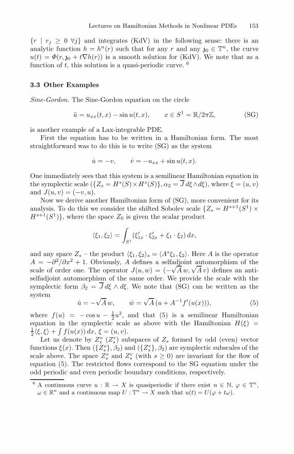
Lectures on Hamiltonian Methods in Nonlinear PDEs 153
r | rj ≥ 0 ∀j and integrates (KdV) in the following sense: there is ananalytic function h = hn(r) such that for any r and any z0 ∈ T
n, the curveu(t) = Φ(r, z0 + t∇h(r)) is a smooth solution for (KdV). We note that as afunction of t, this solution is a quasi-periodic curve. 6
3.3 Other Examples
Sine-Gordon. The Sine-Gordon equation on the circle
u = uxx(t, x)− sinu(t, x), x ∈ S1 = R/2πZ, (SG)
is another example of a Lax-integrable PDE.First the equation has to be written in a Hamiltonian form. The most
straightforward was to do this is to write (SG) as the system
u = −v, v = −uxx + sinu(t, x).
One immediately sees that this system is a semilinear Hamiltonian equation inthe symplectic scale (Zs = Hs(S)×Hs(S), α2 = J dξ∧dξ), where ξ = (u, v)and J(u, v) = (−v, u).
Now we derive another Hamiltonian form of (SG), more convenient for itsanalysis. To do this we consider the shifted Sobolev scale Zs = Hs+1(S1)×Hs+1(S1), where the space Z0 is given the scalar product
〈ξ1, ξ2〉 =∫
S1(ξ′1x · ξ′2x + ξ1 · ξ2) dx,
and any space Zs – the product 〈ξ1, ξ2〉s = 〈Asξ1, ξ2〉. Here A is the operatorA = −∂2/∂x2 + 1. Obviously, A defines a selfadjoint automorphism of thescale of order one. The operator J(u,w) = (−
√Aw,
√Av) defines an anti-
selfadjoint automorphism of the same order. We provide the scale with thesymplectic form β2 = J dξ ∧ dξ. We note that (SG) can be written as thesystem
u = −√Aw, w =
√A (u+A−1f ′(u(x))), (5)
where f(u) = − cosu − 12u
2, and that (5) is a semilinear Hamiltonianequation in the symplectic scale as above with the Hamiltonian H(ξ) =12 〈ξ, ξ〉+
∫
f(u(x)) dx, ξ = (u, v).Let us denote by Zos (Zes ) subspaces of Zs formed by odd (even) vector
functions ξ(x). Then (Zos, β2) and (Zes, β2) are symplectic subscales of thescale above. The space Zos and Zes (with s ≥ 0) are invariant for the flow ofequation (5). The restricted flows correspond to the SG equation under theodd periodic and even periodic boundary conditions, respectively.6 A continuous curve u : R → X is quasiperiodic if there exist n ∈ N, ϕ ∈ T
n,ω ∈ R
n and a continuous map U : Tn → X such that u(t) = U(ϕ+ tω).
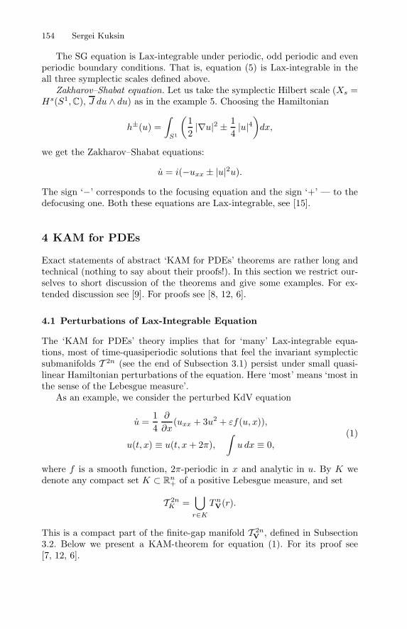
154 Sergei Kuksin
The SG equation is Lax-integrable under periodic, odd periodic and evenperiodic boundary conditions. That is, equation (5) is Lax-integrable in theall three symplectic scales defined above.
Zakharov–Shabat equation. Let us take the symplectic Hilbert scale (Xs =Hs(S1,C), J du ∧ du) as in the example 5. Choosing the Hamiltonian
h±(u) =∫
S1
(12|∇u|2 ± 1
4|u|4)
dx,
we get the Zakharov–Shabat equations:
u = i(−uxx ± |u|2u).
The sign ‘−’ corresponds to the focusing equation and the sign ‘+’ — to thedefocusing one. Both these equations are Lax-integrable, see [15].
4 KAM for PDEs
Exact statements of abstract ‘KAM for PDEs’ theorems are rather long andtechnical (nothing to say about their proofs!). In this section we restrict our-selves to short discussion of the theorems and give some examples. For ex-tended discussion see [9]. For proofs see [8, 12, 6].
4.1 Perturbations of Lax-Integrable Equation
The ‘KAM for PDEs’ theory implies that for ‘many’ Lax-integrable equa-tions, most of time-quasiperiodic solutions that feel the invariant symplecticsubmanifolds T 2n (see the end of Subsection 3.1) persist under small quasi-linear Hamiltonian perturbations of the equation. Here ‘most’ means ‘most inthe sense of the Lebesgue measure’.
As an example, we consider the perturbed KdV equation
u =14∂
∂x(uxx + 3u2 + εf(u, x)),
u(t, x) ≡ u(t, x+ 2π),∫
u dx ≡ 0,(1)
where f is a smooth function, 2π-periodic in x and analytic in u. By K wedenote any compact set K ⊂ R
n+ of a positive Lebesgue measure, and set
T 2nK =
⋃
r∈KT nV(r).
This is a compact part of the finite-gap manifold T 2nV , defined in Subsection
3.2. Below we present a KAM-theorem for equation (1). For its proof see[7, 12, 6].
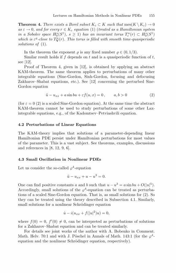
Lectures on Hamiltonian Methods in Nonlinear PDEs 155
Theorem 4. There exists a Borel subset Kε ⊂ K such that mes(K \Kε)→ 0as ε→ 0, and for every r ∈ Kε equation (1) (treated as a Hamiltonian systemin a Sobolev space Hs
0(S1), s ≥ 1) has an invariant torus T nε (r) ⊂ Hs0(S1)
which is ε-close to T nV(r). This torus is filled with smooth time-quasiperiodicsolutions of (1).
In the theorem the exponent is any fixed number ∈ (0, 1/3).Similar result holds if f depends on t and is a quasiperiodic function of t,
see [12].Proof of Theorem 4, given in [12], is obtained by applying an abstract
KAM-theorem. The same theorem applies to perturbations of many otherintegrable equations (Sine-Gordon, Sinh-Gordon, focusing and defocusingZakharov–Shabat equations, etc.). See [12] concerning the perturbed Sine-Gordon equation
u− uxx + a sin bu+ εf(u, x) = 0 , a, b > 0 (2)
(for ε = 0 (2) is a scaled Sine-Gordon equation). At the same time the abstractKAM-theorem cannot be used to study perturbations of some other Lax-integrable equations, e.g., of the Kadomtsev–Petviashvili equation.
4.2 Perturbations of Linear Equations
The KAM-theory implies that solutions of a parameter-depending linearHamiltonian PDE persist under Hamiltonian perturbations for most valuesof the parameter. This is a vast subject. See theorems, examples, discussionsand references in [8, 12, 9, 6].
4.3 Small Oscillation in Nonlinear PDEs
Let us consider the so-called ϕ4-equation
u− uxx + u− u3 = 0.
One can find positive constants a and b such that u− u3 = a sin bu+O(|u|5).Accordingly, small solutions of the ϕ4-equation can be treated as perturba-tions of a scaled Sine-Gordon equation. That is, as small solutions for (2). Sothey can be treated using the theory described in Subsection 4.1. Similarly,small solutions for a nonlinear Schrodinger equation
u− i(uxx + f(|u|2)u) = 0,
where f(0) = 0, f ′(0) = 0, can be interpreted as perturbations of solutionsfor a Zakharov–Shabat equation and can be treated similarly.
For details see joint works of the author with A. Bobenko in Comment.Math. Helv. 70:1 and with J. Poschel in Annals of Math. 143:1 (for the ϕ4-equation and the nonlinear Schrodinger equation, respectively).
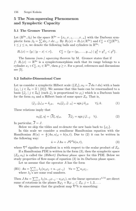
156 Sergei Kuksin
5 The Non-squeezing Phenomenonand Symplectic Capacity
5.1 The Gromov Theorem
Let (R2n, β2) be the space R2n = x1, x−1, . . . , x−n with the Darboux sym-
plectic form β2 =∑dxj ∧ dx−j . By Br(x) = Br(x; R2n) and Cj = Cj(R
2n),1 ≤ j ≤ n, we denote the following balls and cylinders in R
2n:
Br(x) = y | |y − x| < r, Cj = y = (y1, . . . , y−n) | y2j + y2
−j < 2.
The famous (non-) squeezing theorem by M. Gromov states that iff : Br(x) → R
2n is a symplectomorphism such that its range belongs to acylinder x1 +Cj, x1 ∈ R
2n, then ≥ r. For a proof, references and discussionssee [5].
5.2 Infinite-Dimensional Case
Let us consider a symplectic Hilbert scale (Zs, α2 = J du∧ du) with a basisϕj | j ∈ Z0 = Z \ 0. We assume that this basis can be renormalised to abasis ϕj | j ∈ Z0 (each ϕj is proportional to ϕj) which is a Darboux basisfor the form α2 and a Hilbert basis of some space Zd. That is,
〈ϕj , ϕk〉d = δj,k, α2[ϕj , ϕ−k] = sgn j δj,k ∀j, k. (1)
These relations imply that
α2[ξ, η] = 〈Jξ, η〉d, Jϕj = sgn j ϕ−j ∀j. (2)
In particular, J = J .Below we skip the tildes and re-denote the new basis back to ϕj.In this scale we consider a semilinear Hamiltonian equation with the
Hamiltonian H(u) = 12 〈Au, u〉d + h(u, t). Due to (2) it can be written in
the following way:u = JAu + J∇dh(u, t), (3)
where ∇d signifies the gradient in u with respect to the scalar product of Zd.If a Hamiltonian PDE is written in the form (3), then the symplectic space
(Zd, α2) is called the (Hilbert) Darboux phase space for this PDE. Below westudy properties of flow-maps of equation (3) in its Darboux phase space.
Let us assume that the operator A has the form
(H1) Au =∑∞
j=1 λj(ujϕj + u−jϕ−j) ∀u =∑ujϕj ,
where λj ’s are some real numbers.
Then JAu =∑∞
j=1 λj(u−jϕ−j−ujϕj), so the linear operators etJA are directsums of rotations in the planes Rϕj + Rϕ−j ⊂ Zd, j = 1, 2, . . . .
We also assume that the gradient map ∇dh is smoothing:
Lectures on Hamiltonian Methods in Nonlinear PDEs 157
(H2) there exists γ > 0 such that ord∇dh = −γ for s ∈ [d − γ, d + γ].Moreover, the maps
∇dh : Zs × R→ Zs+γ , s ∈ [d− γ, d+ γ],
are C1-smooth and bounded. 7
For any t and T we denote by OTt any open subset of the domain of defini-tion of STt in Zd, such that for each bounded setQ ⊂ OTt the set
⋃
τ∈[t,T ] Sτt (Q)
is bounded in Zd.8
In the theorem below the balls Br and the cylinders Cj, j ≥ 1, are definedin the same way as in Subsection 5.1.
Theorem 5. Let us assume that the assumptions (H1) and (H2) hold andthat a ball Br = Br(u0, Zd) belongs to OTt together with some ε-neighbourhood,ε > 0. Then the relation
STt (Br) ⊂ v0 + Cj(Zd) (4)
with some v0 ∈ Zd and j ≥ 1 implies that ≥ r.
Proof. Without lost of generality we may assume that
v0 = 0, j = 1.
Arguing by contradiction we assume that in (4) < r and choose any 1 ∈(, r).
For n ≥ 1 we denote by E2n the subspace of Zd, spanned by the vectorsϕj , |j| ≤ n, and provide it with the usual Darboux symplectic structure(it is given by the form α2|E2n). By Πn we denote the orthogonal projectionΠn : Zd → E2n. We set
Hn = 12 〈Au, u〉d + h(Πn(u))
and denote by ST(n)t flow-maps of the Hamiltonian vector filed VHn . Any mapST(n)t decomposes to the direct sum of a symplectomorphism of E2n and of alinear symplectomorphism of Zd ! E2n. So the theorem’s assertion with themap STt replaced by ST(n)t follows from the Gromov theorem, applied to thesymplectomorphism
E2n → E2n, x → ΠnST(n)t(i(x) + u0),
where i stands for the embedding of E2n to Zd.7 i.e., they send bounded sets to bounded.8 this set should be treated as a ‘regular part of the domain of definition’.
158 Sergei Kuksin
Lemma 2. Under the theorem’s assumptions the maps ST(n)t are defined onBr for n ≥ n′ with some sufficiently large n′, and there exists a sequenceεn −→
n→∞0 such that
‖STt (u)− ST(n)t(u)‖ ≤ εn (5)
for n ≥ n′ and for every u ∈ Br.
We leave a proof of this lemma as an exercise; alternatively see for theproof [10].
Lemma 3. For any u ∈ Br we have
STt (u) = e(T−t)JAu+ STt (u),
where STt is a C1-smooth map in the scale Zs and ord STt = −γ for s ∈[d− γ, d+ γ].
A proof is another exercise (cf. Lemma 1 in [10]).
Now we continue the proof of the theorem. Since its assertion holds forany map ST(n)t (n ≥ n′) and since the ball Br belongs to this map’s domain ofdefinition (see Lemma 2), then for each n ≥ n′ there exists a point un ∈ Brsuch that ST(n)t(un) /∈ C1
1(0). That is,
|Π1ST(n)t(un)| ≥ 1. (6)
By the weak compactness of a Hilbert ball, we can find a weakly convergingsubsequence
unj u ∈ Br, (7)
sounj → u strongly in Zd−γ .
Due to Lemma 3 this implies that STt (unj )→ STt (u) in Zd, and using (7) weobtain the convergence:
STt (unj ) STt (u). (8)
Noting that |Π1STt (un)| = |Π1S
T(n)tun +Π1(STt − ST(n)t)un| and using (6),
(5) we get:|Π1S
Tt (un)| ≥ 1 − εn, n ≥ n′. (9)
Since by (8) Π1STt (unj ) → Π1S
Tt (u) in E2, then due to (9) we have
|Π1STt (u)| ≥ 1. This contradicts (4) because 1 > . The obtained contra-
diction proves the theorem.
Lectures on Hamiltonian Methods in Nonlinear PDEs 159
5.3 Examples
Example 7. Let us consider the nonlinear wave equation
u = ∆u− f(u; t, x), (10)
where u = u(t, x), x ∈ Tn. The function f is a polynomial in u of a degree D
such that its coefficients are smooth functions of t and x. We set f = f − u,denote by B the linear operator B =
√1−∆ and write (10) as the system of
two equations:u = −Bv,v = Bu+B−1f(u; t, x).
(11)
Let us take for Zs the shifted Sobolev scale Zs = Hs+1/2(Tn; R2), where〈ξ, η〉s =
∫
Tn B2s+1ξ · η dx.
Taking for α2 the Darboux form α2 = J dξ ∧ dξ, where Jξ = (−v, u) forξ = (u, v), one sees that (11) is a Hamiltonian equation with the Hamiltonian
H(u, v) =12〈B(u, v), (u, v)〉0 +
∫
F (u; t, x) dx,
where F ′u = f0. Choosing for ψj | j ∈ N a (properly enumerated) Hilbert
basis of the space H1/2(Tn), formed by functions CsRe eis·x and Cs Im eis·x,we set
ϕj = (ψj , 0), ϕ−j = (0, ψj), j ∈ N.
The basis ϕj satisfies (1), so Z0 = H1/2(Tn,R2) is the Darboux phase spacefor the nonlinear wave equation, written in the form (11).
To apply Theorem 5 we have to check conditions (H1) and (H2). The firstone (with A = B) holds trivially since ϕj ’s are eigenfunctions of the Laplacian.The condition (H2) holds in the following three cases:
a) n = 1,b) n = 2, D ≤ 4,c) n = 3, D ≤ 2.The case a) and the case b) with D ≤ 2 can be checked using elementary
tools, see [10]. Arguments in the case b) with 3 ≤ D ≤ 4 and in the case c)are based on Strichartz-type inequalities, see [3].
In the cases a)–c), Theorem 5 applies to equation (10) in the form (11) andshows that the flow maps cannot squeeze H1/2-balls to narrow cylinders. Thisresult can be interpreted as impossibility of ‘locally uniform’ energy transitionto high modes, see [10].
Example 8. For a nonlinear Schrodinger equation
u = i∆u+ if ′u(|u|2)u, x ∈ T
n (12)
(cf. Example 4), the Darboux phase space is the L2-space L2(Tn; C). It is veryunlikely that the flow-maps of (12) satisfy in this space assumption (H2). Sowe smooth out the Hamiltonian of (12) and replace it by
160 Sergei Kuksin
Hξ =12
∫
(|∇u|2 + f(|U |2)) dx, U = u ∗ ξ,
where u ∗ ξ is the convolution of u with a function ξ ∈ C∞(Tn,R). Thecorresponding Hamiltonian equation is
u = i∆u+ i(f ′(|U |2)U) ∗ ξ.
This smoothed equation satisfies (H1), (H2) and Theorem 5 applies to itsflow-maps.
5.4 Symplectic Capacity
Another way to prove Theorem 5 uses a new object — symplectic capacity —which is interesting on its own.
Symplectic capacity in a Hilbert Darboux space (Zd, α2) as in Subsection5.2 (below we abbreviate Zd to Z), is a map c which corresponds to any opensubset O ⊂ Z a number c(O) ∈ [0,∞] and satisfies the following properties:
1) translational invariance: c(O) = c(O + ξ) for any ξ ∈ Z;2) monotonicity: if O1 ⊃ O2, then c(O1) ≥ c(O2);3) 2-homogeneity: c(τO) = τ2c(O);4) normalisation: for any ball Br = Br(x;Z) and any cylinder Cjr = Cjr (Z)
we havec(Br) = c(Cjr ) = πr2.
(We note that for x = 0 the cylinder contains the ball and is ‘much bigger’,but both sets have the same capacity.)
5) Symplectic invariance: for any symplectomorphism Φ : Z → Z and anydomain O, c(Φ(O)) = c(O).
If (Z,α2) is a finite-dimensional Darboux space, then existence of a capac-ity with properties 1)–5) is equivalent to the Gromov theorem. Indeed, if acapacity exists, then the squeezing (4) with < r is impossible due to 2), 4)and 5). On the opposite, the quantity
c(O) = supπr2 | there exists a symplectomorphism which sends Br in O
obviously satisfies 1)–3) and 5). Using the Gromov theorem we see that csatisfies 4) as well.
If (Z,α2) is a Hilbert Darboux space, then the finite-dimensional sym-plectic capacity, obtained in [5], can be used to construct a capacity c whichmeets 1)–4). This capacity turns out to be invariant under symplectomor-phisms, which are flow-maps STt as in Theorem 5, see [10]. This result alsoimplies Theorem 5.
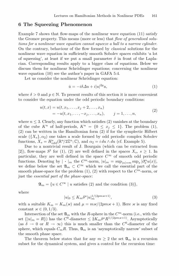
Lectures on Hamiltonian Methods in Nonlinear PDEs 161
6 The Squeezing Phenomenon
Example 7 shows that flow-maps of the nonlinear wave equation (11) satisfythe Gromov property. This means (more or less) that flow of generalised solu-tions for a nonlinear wave equation cannot squeeze a ball to a narrow cylinder.On the contrary, behaviour of the flow formed by classical solutions for thenonlinear wave equation in sufficiently smooth Sobolev spaces exhibits ‘a lotof squeezing’, at least if we put a small parameter δ in front of the Lapla-cian. Corresponding results apply to a bigger class of equations. Below wediscuss them for nonlinear Schrodinger equations; concerning the nonlinearwave equation (10) see the author’s paper in GAFA 5:4.
Let us consider the nonlinear Schrodinger equation:
u = −iδ∆u+ i|u|2pu, (1)
where δ > 0 and p ∈ N. To present results of this section it is more convenientto consider the equation under the odd periodic boundary conditions:
u(t, x) = u(t, x1, . . . , xj + 2, . . . , xn)= −u(t, x1, . . . ,−xj , . . . , xn), j = 1, . . . , n,
(2)
where n ≤ 3. Clearly, any function which satisfies (2) vanishes at the boundaryof the cube Kn of half-periods, Kn = 0 ≤ xj ≤ 1. The problem (1),(2) can be written in the Hamiltonian form (2) if for the symplectic Hilbertscale (Xs, α2) one takes a scale formed by odd periodic complex Sobolevfunctions, Xs = Hs
odd(Rn/2Z
n; C), and α2 = i du ∧ du (cf. Example 5).Due to a nontrivial result of J. Bourgain (which can be extracted from
[2]), flow-maps St for (1), (2) are well defined in the spaces Xs, s ≥ 1. Inparticular, they are well defined in the space C∞ of smooth odd periodicfunctions. Denoting by | · |m the Cm-norm, |u|m = sup|α|=m supx |∂αx u(x)|,we define below the set Am ⊂ C∞ which we call the essential part of thesmooth phase-space for the problem (1), (2) with respect to the Cm-norm, orjust the essential part of the phase-space:
Am = u ∈ C∞ | u satisfies (2) and the condition (3),
where|u|0 ≤ Kmδ
µ|u|1/(2pmκ+1)m , (3)
with a suitable Km = Km(κ) and µ = mκ/(2pmκ + 1). Here κ is any fixedconstant κ ∈ (0, 1/3).
Intersection of the set Am with the R-sphere in the Cm-norm (i.e., with theset |u|m = R) has the C0-diameter ≤ 2Kmδ
µR1/(2pmκ+1). Asymptotically(as δ → 0 or R → ∞) this is much smaller than the C0-diameter of thesphere, which equals CmR. Thus, Am is an ‘asymptotically narrow’ subset ofthe smooth phase space.
The theorem below states that for any m ≥ 2 the set Am is a recursionsubset for the dynamical system, and gives a control for the recursion time:
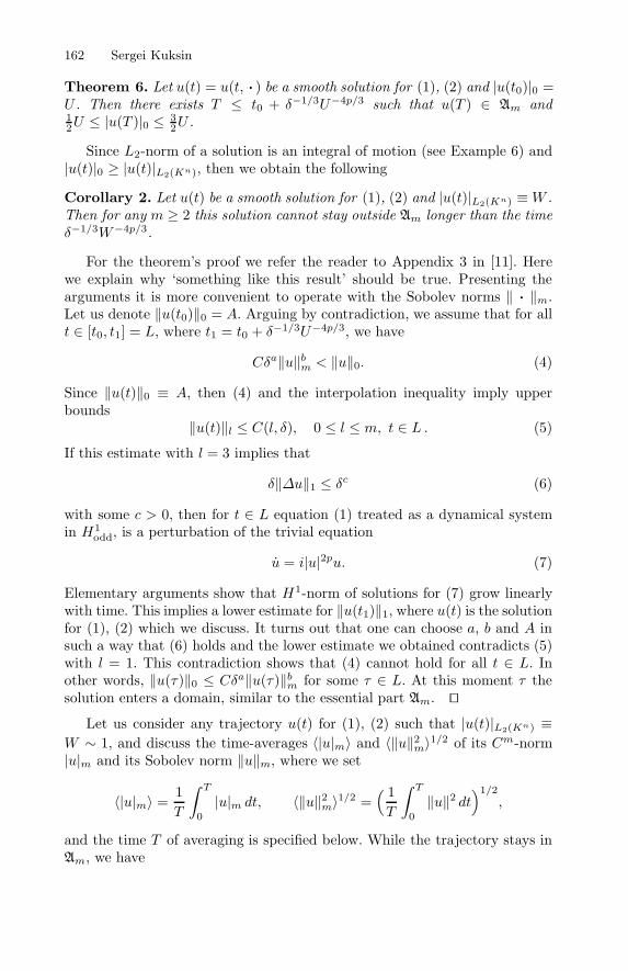
162 Sergei Kuksin
Theorem 6. Let u(t) = u(t, · ) be a smooth solution for (1), (2) and |u(t0)|0 =U . Then there exists T ≤ t0 + δ−1/3U−4p/3 such that u(T ) ∈ Am and12U ≤ |u(T )|0 ≤ 3
2U .
Since L2-norm of a solution is an integral of motion (see Example 6) and|u(t)|0 ≥ |u(t)|L2(Kn), then we obtain the following
Corollary 2. Let u(t) be a smooth solution for (1), (2) and |u(t)|L2(Kn) ≡W .Then for any m ≥ 2 this solution cannot stay outside Am longer than the timeδ−1/3W−4p/3.
For the theorem’s proof we refer the reader to Appendix 3 in [11]. Herewe explain why ‘something like this result’ should be true. Presenting thearguments it is more convenient to operate with the Sobolev norms ‖ · ‖m.Let us denote ‖u(t0)‖0 = A. Arguing by contradiction, we assume that for allt ∈ [t0, t1] = L, where t1 = t0 + δ−1/3U−4p/3, we have
Cδa‖u‖bm < ‖u‖0. (4)
Since ‖u(t)‖0 ≡ A, then (4) and the interpolation inequality imply upperbounds
‖u(t)‖l ≤ C(l, δ), 0 ≤ l ≤ m, t ∈ L . (5)
If this estimate with l = 3 implies that
δ‖∆u‖1 ≤ δc (6)
with some c > 0, then for t ∈ L equation (1) treated as a dynamical systemin H1
odd, is a perturbation of the trivial equation
u = i|u|2pu. (7)
Elementary arguments show that H1-norm of solutions for (7) grow linearlywith time. This implies a lower estimate for ‖u(t1)‖1, where u(t) is the solutionfor (1), (2) which we discuss. It turns out that one can choose a, b and A insuch a way that (6) holds and the lower estimate we obtained contradicts (5)with l = 1. This contradiction shows that (4) cannot hold for all t ∈ L. Inother words, ‖u(τ)‖0 ≤ Cδa‖u(τ)‖bm for some τ ∈ L. At this moment τ thesolution enters a domain, similar to the essential part Am.
Let us consider any trajectory u(t) for (1), (2) such that |u(t)|L2(Kn) ≡W ∼ 1, and discuss the time-averages 〈|u|m〉 and 〈‖u‖2m〉1/2 of its Cm-norm|u|m and its Sobolev norm ‖u‖m, where we set
〈|u|m〉 =1T
∫ T
0
|u|m dt, 〈‖u‖2m〉1/2 =( 1T
∫ T
0
‖u‖2 dt)1/2
,
and the time T of averaging is specified below. While the trajectory stays inAm, we have
Lectures on Hamiltonian Methods in Nonlinear PDEs 163
|u|m ≥ (WK−1m δ−µ)1/(1−2pµ).
One can show that this inequality implies that each visit to Am increasesthe integral
∫
|u|m dt by a term bigger than δ to a negative degree. Sincethese visits are sufficiently frequent by the Corollary, then we obtain a lowerestimate for the quantity 〈|u|m〉. Details can be found in the author’s paperin CMPh 178, pp. 265–280. Here we present a better result which estimatesthe time-averaged Sobolev norms. For a proof see Subsection 4.1 of [11].
Theorem 7. Let u(t) be a smooth solution for the equation (1), (2) suchthat |u(t)|L2(Kn) ≥ 1. Then there exists a sequence km 1/3 and constantsCm > 0, δm > 0 such that 〈‖u‖2m〉1/2 ≥ Cmδ
−2mkm , provided that m ≥ 4,δ ≤ δm and T ≥ δ−1/3.
The results stated in Theorems 6, 7 remain true for equations (1) withdissipation. I.e., for the equations with δ replaced by δν, where ν is a unitcomplex number such that Re ν ≥ 0 and Im ν ≥ 0. 9 If Im ν > 0, then smoothsolutions for (1), (2) converge to zero in any Cm-norm. Since the essentialpart Am clearly contains a sufficiently small Cm-neighbourhood of zero, theneventually any smooth solution enter Am and stays there forever. Theorem(1) states that the solution will visit the essential part much earlier, before itsnorm decays.
References
1. V. I. Arnold. Mathematical methods in classical mechanics. Springer-Verlag,Berlin, 3rd edition, 1989.
2. J. Bourgain. Fourier transform restriction phenomenona for certain lattice sub-sets and applications to nonlinear evolution equations. Geometric and Func-tional Analysis, 3:107–156 and 209–262, 1993.
3. J. Bourgain. Aspects of long time behaviour of solutions of nonlinear Hamilto-nian evolution equations. Geometric and Functional Analysis, 5:105–140, 1995.
4. G. E. Giacaglia. Perturbation methods in non-linear systems. Springer-Verlag,Berlin, 1972.
5. H. Hofer and E. Zehnder. Symplectic invariants and Hamiltonian dynamics.Birkhauser, Basel, 1994.
6. T. Kappeler and J. Poschel. Perturbed KdV equation, 2001.7. S. B. Kuksin. The perturbation theory for the quasiperiodic solutions of infinite-
dimensional hamiltonian systems and its applications to the Korteweg – de Vriesequation. Math. USSR Sbornik, 64:397–413, 1989.
8. S. B. Kuksin. Nearly integrable infinite-dimensional Hamiltonian Systems.Springer-Verlag, Berlin, 1993.
9. S. B. Kuksin. KAM-theory for partial differential equations. In Proceed-ings of the First European Congress of Mathematics, volume 2, pages 123–157.Birkhauser, 1994.
9 The only correction is that if Im ν > 0, then in Theorem 7 one should takeT = δ−1/3.
164 Sergei Kuksin
10. S. B. Kuksin. Infinite-dimensional symplectic capacities and a squeezing theoremfor Hamiltonian PDEs. Comm. Math. Physics, 167:531–552, 1995.
11. S. B. Kuksin. Spectral properties of solutions for nonlinear PDEs in the turbu-lent regime. Geometric and Functional Analysis, 9:141–184, 1999.
12. S. B. Kuksin. Analysis of Hamiltonian PDEs. Oxford University Press, Oxford,2000.
13. A. Pazy. Semigroups of linear operators and applications to partial differentialequations. Springer-Verlag, Berlin, 1983.
14. M. Reed and B. Simon. Methods of modern mathematical physics, volume 2.Academic Press, New York - London, 1975.
15. V. E. Zakharov, S. V. Manakov, S. P. Novikov, and L. P. Pitaevskij. Theory ofsolitons. Plenum Press, New York, 1984.
List of Participants
1. Berretti AlbertoDipartimento di Matematica, II Universita’ di Roma (Tor Vergata),via della Ricerca scientifica, 00133 Roma (Italy)[email protected]
2. Benettin GiancarloDipartimento di Matematica Pura ed Applicata,Universita’ di Padova,via Belzoni 7, 35131 Padova (Italy)[email protected]
3. Bertini MassimoDipartimento di Matematica, Universita’ Statale di Milano,via Saldini 50, 20133 Milano (Italy)[email protected]
4. Bertotti Maria LetiziaDipartimento di Matematica e Applicazioni c/o Ingegneria,Viale delle Scienze, 90128 Palermo (Italy) and:Dipartimento Ingegneria Meccanica e Strutturale, Ingegneria,via Mesiano 77, 38050 Trento (Italy)[email protected] [email protected]
5. Camyshev AndreiInstitute of Mathematics,Akademijas lauk. 1, Riga, LV 1524 (Latvia)[email protected]
6. Castella EnricDepartament de Matematica Aplicada i Analisi,Universitat de Barcelona,Gran Via 585, 08007 Barcelona (Spain)[email protected]
7. Cellina ArrigoDipartimento di Matematica e Applicazioni,Universita’ di Milano Bicocca,via degli Arcimboldi 8, 20126 Milano, (Italy)[email protected]
166 List of Participants
8. Cherubini Anna MariaDipartimento di Matematica, Universita’ degli Studi di Lecce,via per Arnesano, 73100 Lecce (Italy)[email protected]
9. Conti MonicaDipartimento di Matematica del Politecnico di Milano,Piazza Leonardo da Vinci 32, Milano (Italy)[email protected] [email protected]
10. Degiovanni LucaDipartimento di Matematica, Universita’ di Torino,Palazzo Campana, via Carlo Albrto, Torino (Italy)[email protected]
11. Eliasson HakanDepartment of Mathematics, Royal Inst. of Techn.S-10044 Stockolm (Sweden)[email protected]
12. Fasso FrancescoDipartimento di Matematica Pura ed Applicata, Universita’ di Padova,via Belzoni 7, 35131 Padova (Italy)[email protected]
13. Finco DomenicoDipartimento di Matematica, Universita’ ”La Sapienza” di Romapiazza A. Moro 5, 00185 Roma (Italy)[email protected]
14. Firpo Marie ChristinePIIM - UMR 6633, Equipe Turbulece Plasma,Universite’ Aix-Marseille ICentre S. Jerome, Case 321-F-13397,Marseille Cedex 20 (France)[email protected]
15. Gabern FredericDepartament de Matematica Aplicada i Analisi, Universitat de Barcelona,Gran Via 585, 08007 Barcelona (Spain)[email protected]
16. Galgani LuigiDipartimento di Matematica, Universita’ Statale di Milano,via Saldini 50, 20133 Milano (Italy)[email protected]
17. Gentile GuidoDipartimento di Matematica, Universita’ di Roma 3,Largo S. Leonardo Murialdo 1, 00146 Roma (Italy)[email protected]
List of Participants 167
18. Giorgi GiordanoDepartment: Dipartimento di Fisica, Universita’ ”La Sapienza”Personal Post Address: via G. Sirtori 69, 00149 Roma (Italy)[email protected]
19. Giorgilli AntonioDipartimento di Matematica e Applicazioni,Universita’ di Milano Bicocca,via degli Arcimboldi 8, 20126 Milano (Italy)[email protected]
20. Gonzalez Maria AlejandraDepartament de Matematica Aplicada i Analisi,Universitat de Barcelona,Gran Via 585, 08007 Barcelona (Spain)[email protected]
21. Henrard JacquesDepartement de Mathematique FUNDP 8,Rempart de la Vierge, B-5000 Namur, (Belgium)[email protected]
22. Kuksin SergeiDepartment of Mathematics, Heriott-Watt University,Edinburgh EH14 4AS, Scotland (United Kingdom)[email protected]
23. Lazaro Ochoa J.TomasDepartament de Matematica Aplicada I,Universitat Politecnica de Catalunya,Diagonal 647, 08028 Barcelona (Spain)[email protected]
24. Locatelli UgoSchool of Cosmic Physics, Dublin Institut for Advanced Studies,5 Merrion Square, Dublin 2, (Ireland)[email protected]
25. Macri’ MartaDipartimento di Matematica e Applicazioni ”R. Cacciopoli”,Monte S. Angelo, via Cinthia, Napoli (Italy)[email protected]
26. Mastropietro VieriDipartimento di Matematica,II Universita’ di Roma (Tor Vergata),via della Ricerca scientifica, 00133 Roma (Italy)[email protected]
27. Naselli FranzDepartament de Matematica Aplicada i Analisi,Universitat de Barcelona,Gran Via 585, 08007 Barcelona (Spain)[email protected]
168 List of Participants
28. Nekhoroshev NikolaiDepartment of Mechanics and Mathematics, Moscow State University,119899 Moscow (Russia)[email protected]
29. Pacha Andujar Juan RamonDepartament de Matematica Aplicada I,Universitat Politecnica de Catalunya,Diagonal 647, 08028 Barcelona (Spain)[email protected]
30. Paleari SimoneDipartimento di Matematica, Universita’ Statale di Milano,via Saldini 50, 20133 Milano, (Italy)[email protected]
31. Panati GianlucaMathematical Physics Sector, SISSA/ISAS,via Beirut 2, 34014 Trieste (Italy)[email protected]
32. Prykarpatsky YaremaDepartment of ordinary differential equations,Institute of Mathematics at MAS of Ukraine,Tereshchenkirska str., 252601 Kiev (Ukraine)[email protected]
33. Puig JoaquimDepartament de Matematica Aplicada i Analisi,Universitat de Barcelona,Gran Via 585, 08007 Barcelona (Spain)[email protected]
34. Pyke RandallDepartment of Mathematics, University of Toronto,Toronto, Ontario, M5S 3G3 (Canada)[email protected]
35. Sama Cami AnnaDepartament de Matematiques, Facultat de Ciencies,Universitat Autonoma de Barcelona08290 Cerdanyola del Valles (Spain)[email protected]
36. Shirikyan ArmenDepartment of Mathematics, Heriott-Watt University,Edinburgh EH14 4AS, Scotland (United Kingdom)[email protected]
37. Simo’ CarlesDepartament de Matematica Aplicada i Analisi,Universitat de Barcelona,Gran Via 585, 08007 Barcelona (Spain)[email protected]
List of Participants 169
38. Slijepcevic SinisaDepartment of Mathematics, PMF,Bijenicka 30, 10000 Zagreb (Croatia)[email protected]
39. Sommer BrittaInst. Reine und Angewandte Mathematik,RWTH-Aachen Templergraben 55, 52062 Aachen (Germany)[email protected]
40. Terracini SusannaDipartimento di Matematica del Politecnico di Milano,Piazza Leonardo da Vinci 32, Milano (Italy)[email protected]
41. Villanueva JordiDepartament de Matematica Aplicada I,Universitat Politecnica de Catalunya,Diagonal 647, 08028 Barcelona (Spain)[email protected]
42. Vitolo RenatoDepartment of Mathematics, University of Groningen,P.O. Box 800, 9700 AV Groningen (Netherlands)[email protected]
43. Vittot MichelCentre de Physique theorique - CNRSLuminy, Case 907, 13288 Marseille, Cedex 9 (France)[email protected]

LIST OF C.I.M.E. SEMINARS
1954 1. Analisi funzionale C.I.M.E
2. Quadratura delle superficie e questioni connesse "
3. Equazioni differenziali non lineari "
1955 4. Teorema di Riemann-Roch e questioni connesse "
5. Teoria dei numeri "
6. Topologia "
7. Teorie non linearizzate in elasticita,idrodinamica, aerodinamic
"
8. Geometria proiettivo-differenziale "
1956 9. Equazioni alle derivate parziali a caratteristichereali
"
10. Propagazione delle onde elettromagnetiche "
11. Teoria della funzioni di piu variabili complesse edelle funzioni automorfe
"
1957 12. Geometria aritmetica e algebrica (2 vol.) "
13. Integrali singolari e questioni connesse "
14. Teoria della turbolenza (2 vol.) "
1958 15. Vedute e problemi attuali in relativita generale "
16. Problemi di geometria differenziale in grande "
17. Il principio di minimo e le sue applicazioni alleequazioni funzionali
"
1959 18. Induzione e statistica "
19. Teoria algebrica dei meccanismi automatici (2 vol.) "
20. Gruppi, anelli di Lie e teoria della coomologia "
1960 21. Sistemi dinamici e teoremi ergodici "
22. Forme differenziali e loro integrali "
1961 23. Geometria del calcolo delle variazioni (2 vol.) "
24. Teoria delle distribuzioni "
25. Onde superficiali "
1962 26. Topologia differenziale "
27. Autovalori e autosoluzioni "
28. Magnetofluidodinamica "
1963 29. Equazioni differenziali astratte "
30. Funzioni e varieta complesse "
31. Proprieta di media e teoremi di confronto inFisica Matematica
"
1964 32. Relativita generale "
33. Dinamica dei gas rarefatti "
34. Alcune questioni di analisi numerica "
35. Equazioni differenziali non lineari "
1965 36. Non-linear continuum theories "
37. Some aspects of ring theory "
38. Mathematical optimization in economics "
172 LIST OF C.I.M.E. SEMINARS
1966 39. Calculus of variations Ed. Cremonese, Firenze
40. Economia matematica "
41. Classi caratteristiche e questioni connesse "
42. Some aspects of diffusion theory "
1967 43. Modern questions of celestial mechanics "
44. Numerical analysis of partial differentialequations
"
45. Geometry of homogeneous bounded domains "
1968 46. Controllability and observability "
47. Pseudo-differential operators "
48. Aspects of mathematical logic "
1969 49. Potential theory "
50. Non-linear continuum theories in mechanics andphysics and their applications
"
51. Questions of algebraic varieties "
1970 52. Relativistic fluid dynamics "
53. Theory of group representations and Fourieranalysis
"
54. Functional equations and inequalities "
55. Problems in non-linear analysis "
1971 56. Stereodynamics "
57. Constructive aspects of functional analysis (2 vol.) "
58. Categories and commutative algebra "
1972 59. Non-linear mechanics "
60. Finite geometric structures and their applications "
61. Geometric measure theory and minimal surfaces "
1973 62. Complex analysis "
63. New variational techniques in mathematicalphysics
"
64. Spectral analysis "
1974 65. Stability problems "
66. Singularities of analytic spaces "
67. Eigenvalues of non linear problems "
1975 68. Theoretical computer sciences "
69. Model theory and applications "
70. Differential operators and manifolds "
1976 71. Statistical Mechanics Ed. Liguori, Napoli
72. Hyperbolicity "
73. Differential topology "
1977 74. Materials with memory "
75. Pseudodifferential operators with applications "
76. Algebraic surfaces "
1978 77. Stochastic differential equations Ed. Liguori, Napoli& Birkhauser
78. Dynamical systems "
1979 79. Recursion theory and computational complexity "
80. Mathematics of biology "
1980 81. Wave propagation "
82. Harmonic analysis and group representations "
83. Matroid theory and its applications "
LIST OF C.I.M.E. SEMINARS 173
1981 84. Kinetic Theories and the Boltzmann Equation (LNM 1048) Springer-Verlag
85. Algebraic Threefolds (LNM 947) "
86. Nonlinear Filtering and Stochastic Control (LNM 972) "
1982 87. Invariant Theory (LNM 996) "
88. Thermodynamics and Constitutive Equations (LN Physics 228) "
89. Fluid Dynamics (LNM 1047) "
1983 90. Complete Intersections (LNM 1092) "
91. Bifurcation Theory and Applications (LNM 1057) "
92. Numerical Methods in Fluid Dynamics (LNM 1127) "
1984 93. Harmonic Mappings and Minimal Immersions (LNM 1161) "
94. Schrodinger Operators (LNM 1159) "
95. Buildings and the Geometry of Diagrams (LNM 1181) "
1985 96. Probability and Analysis (LNM 1206) "
97. Some Problems in Nonlinear Diffusion (LNM 1224) "
98. Theory of Moduli (LNM 1337) "
1986 99. Inverse Problems (LNM 1225) "
100. Mathematical Economics (LNM 1330) "
101. Combinatorial Optimization (LNM 1403) "
1987 102. Relativistic Fluid Dynamics (LNM 1385) "
103. Topics in Calculus of Variations (LNM 1365) "
1988 104. Logic and Computer Science (LNM 1429) "
105. Global Geometry and Mathematical Physics (LNM 1451) "
1989 106. Methods of nonconvex analysis (LNM 1446) "
107. Microlocal Analysis and Applications (LNM 1495) "
1990 108. Geometric Topology: Recent Developments (LNM 1504) "
109. H∞ Control Theory (LNM 1496) "
110. Mathematical Modelling of Industrial Processes (LNM 1521) "
1991 111. Topological Methods for Ordinary DifferentialEquations
(LNM 1537) "
112. Arithmetic Algebraic Geometry (LNM 1553) "
113. Transition to Chaos in Classical and QuantumMechanics
(LNM 1589) "
1992 114. Dirichlet Forms (LNM 1563) "
115. D-Modules, Representation Theory, andQuantum Groups
(LNM 1565) "
116. Nonequilibrium Problems in Many-ParticleSystems
(LNM 1551) "
1993 117. Integrable Systems and Quantum Groups (LNM 1620) "
118. Algebraic Cycles and Hodge Theory (LNM 1594) "
119. Phase Transitions and Hysteresis (LNM 1584) "
1994 120. Recent Mathematical Methods in NonlinearWave Propagation
(LNM 1640) "
121. Dynamical Systems (LNM 1609) "
122. Transcendental Methods in Algebraic Geometry (LNM 1646) "
1995 123. Probabilistic Models for Nonlinear PDE’s (LNM 1627) "
124. Viscosity Solutions and Applications (LNM 1660) "
125. Vector Bundles on Curves. New Directions (LNM 1649) "
174 LIST OF C.I.M.E. SEMINARS
1996 126. Integral Geometry, Radon Transforms andComplex Analysis
(LNM 1684) Springer-Verlag
127. Calculus of Variations and Geometric EvolutionProblems
(LNM 1713) "
128. Financial Mathematics (LNM 1656) "
1997 129. Mathematics Inspired by Biology (LNM 1714) "
130. Advanced Numerical Approximation of NonlinearHyperbolic Equations
(LNM 1697) "
131. Arithmetic Theory of Elliptic Curves (LNM 1716) "
132. Quantum Cohomology (LNM 1776) "
1998 133. Optimal Shape Design (LNM 1740) "
134. Dynamical Systems and Small Divisors (LNM 1784) "
135. Mathematical Problems in SemiconductorPhysics
(LNM 1823) "
136. Stochastic PDE’s and Kolmogorov Equations inInfinite Dimension
(LNM 1715) "
137. Filtration in Porous Media and IndustrialApplications
(LNM 1734) "
1999 138. Computational Mathematics driven by IndustrialApplications
(LNM 1739) "
139. Iwahori-Hecke Algebras and RepresentationTheory
(LNM 1804) "
140. Hamiltonian Dynamics - Theory and Applications (LNM 1861) "
141. Global Theory of Minimal Surfaces in Flat Spaces (LNM 1775) "
142. Direct and Inverse Methods in Solving NonlinearEvolution Equations
(LNP 632) "
2000 143. Dynamical Systems (LNM 1822) "
144. Diophantine Approximation (LNM 1819) "
145. Mathematical Aspects of Evolving Interfaces (LNM 1812) "
146. Mathematical Methods for Protein Structure (LNCS 2666) "
147. Noncommutative Geometry (LNM 1831) "
2001 148. Topological Fluid Mechanics to appear "
149. Spatial Stochastic Processes (LNM 1802) "
150. Optimal Transportation and Applications (LNM 1813) "
151. Multiscale Problems and Methods in NumericalSimulations
(LNM 1825) "
2002 152. Real Methods in Complex and CR Geometry (LNM 1848) "
153. Analytic Number Theory to appear "
154. Imaging to appear "
2003 155. Stochastic Methods in Finance (LNM 1856) "
156. Hyperbolic Systems of Balance Laws to appear "
157. Symplectic 4-Manifolds and Algebraic Surfaces to appear "
158. Mathematical Foundation of Turbulent ViscousFlows
to appear "
2004 159. Representation Theory and Complex Analysis to appear "
160. Nonlinear and Optimal Control Theory to appear "
161. Stochastic Geometry to appear "
LIST OF C.I.M.E. SEMINARS 175
2005 162. Enumerative Invariants in Algebraic Geometryand String Theory
announced Springer-Verlag
163. Calculus of Variations and Non-linear PartialDifferential Equations
announced "
164. SPDE in Hydrodynamics: Recent Progress andProspects
announced "
Fondazione C.I.M.E.
Centro Internazionale Matematico EstivoInternational Mathematical Summer Center
http://[email protected]
2005 COURSES LIST
Enumerative Invariantsin Algebraic Geometry and String Theory
June 6–11, Cetraro
Course Directors:Prof. Kai Behrend (University of British Columbia, Vancouver, Canada)Prof. Barbara Mantechi (SISSA, Trieste, Italy)
Calculus of Variationsand Non-linear Partial Differential Equations
June 27–July 2, Cetraro
Course Directors:Prof. Bernard Dacorogna (EPFL, Lousanne, Switzerland)Prof. Paolo Marcellini (Universita di Firenze, Italy)
SPDE in Hydrodynamics:Recent Progress and Prospects
August 29–September 3, Cetraro
Course Directors:Prof. Giuseppe Da Prato (Scuola Normale Superiore, Pisa, Italy)Prof. Michael Rockner (Bielefeld University, Germany)