Lecture Notes in Contract Theory - NYUhmueller/papers/Ch1to4.pdf · Lecture Notes in Contract Theory Holger M. Müller Stockholm School of Economics May 1997 preliminary and incomplete

Lecture Notes in Contract Theory

Holger M. MüllerStockholm School of Economics

May 1997

preliminary and incomplete

Contents

1 Introduction 3

2 Mechanism Design 52.1 The Implementation Problem . . . . . . . . . . . . . . . . . . 52.2 Dominant Strategy Implementation . . . . . . . . . . . . . . . 112.3 Nash Implementation . . . . . . . . . . . . . . . . . . . . . . . 212.4 Bayesian Implementation . . . . . . . . . . . . . . . . . . . . . 272.5 Bibliographic Notes . . . . . . . . . . . . . . . . . . . . . . . . 452.6 References . . . . . . . . . . . . . . . . . . . . . . . . . . . . . 46

3 Adverse Selection 483.1 Static Adverse Selection . . . . . . . . . . . . . . . . . . . . . 483.2 Repeated Adverse Selection . . . . . . . . . . . . . . . . . . . 603.3 Bibliographic Notes . . . . . . . . . . . . . . . . . . . . . . . . 683.4 References . . . . . . . . . . . . . . . . . . . . . . . . . . . . . 68

4 Moral Hazard 694.1 Static Moral Hazard . . . . . . . . . . . . . . . . . . . . . . . 694.2 Extensions: Multiple Signals, Multiple Agents, and Multiple

Tasks . . . . . . . . . . . . . . . . . . . . . . . . . . . . . . . . 87

2

Chapter 1

Introduction

Common sense suggests that contracts which are not enforceable are notworth the paper on which they are written. Enforcement, however, requiresboth the existence of a functioning legal system and the ability of courts tojudge whether a contract has been broken. The latter criterion leads directlyto the notion of verifiability. If the performance of a contractual duty is notverifiable vis-a-vis the court, then we can reasonably assume that this dutyis not enforceable, which in turn implies that it should not be made part ofa contract in the first place.In many situations, parties would like to include a rule or instruction in

a contract, but cannot do so by the above reasoning because either i) theperformance of the rule is observable by all parties but not verifiable vis-a-vis the court, or ii) the performance is not even observable by all the partiesinvolved. Throughout these notes, we refer to such rules as social choicerules. A social choice rule is a mapping f : Θ → A from a set of states Θinto a set of outcomes or alternatives A. While we exclusively concentrate onsocial choice rules that are (Pareto-)efficient, we abstract from distributionalconsequences. For instance, in chapters 3 and 4, we deal with social choicerules that maximize the (expected) utility of one party subject to holding theutility of another party constant at the lowest possible level. This suggeststhat the term ”social” must not always be taken literally.Contract theory is concerned with the implementation of social choice

rules in situations where these cannot be made part of a contract due tothe presence of incomplete information (i.e. either non-observability and/ornon-verifiability of performance). In such cases, we examine whether thesocial choice rule in question can be implemented indirectly or replicatedthrough either a) an alternative rule that is enforceable by courts or b) someinstitutional arrangement. If the social choice rule can be fully replicated,then we speak of an efficient or first-best solution. Usually, however, this

3

CHAPTER 1. INTRODUCTION 4

is not possible due to the constraints imposed by incomplete information.We then typically search for an enforceable alternative rule or institutionalarrangement that maximizes potential efficiency gains and thus comes asclose as possible to the original social choice rule. Such rules or institutionsare called constrained efficient or second-best optimal.In chapters 2 to 4, we study contracts (i.e. rules or instructions) that

are comprehensive in the sense that they optimally take into account allcommonly observable information. There, it is implicitly assumed that thisinformation is also verifiable in front of courts. Often, however, it is too costlyto write a contract that is contingent on all jointly observable information.For instance, suppose that an employment contract had to specificy what abricklayer should do next Monday when the weather is x, his health is y, andthe price of concrete is z. If each of these three variables had only ten possiblerealizations, the contract would have to include 1,000 different contingencies.Alternatively, some commonly observable information may simply not beverifiable vis-a-vis the court. In both cases, contracts will be left incomplete,i.e. they will not optimally utilize all available information. Incompletecontracts are the subject of chapter 5. When the incompleteness is severesuch that there is no hope of replicating the SCR through an alternativeenforceable rule, institutional arrangements become important. In the caseof the bricklayer, we would expect that either he or his supervisor has theauthority do decide what to do in each situation. If (nonhuman) assetsare involved, ownership rights usually determine how the asset is used inunforeseen contingencies.

To be completed

Chapter 2

Mechanism Design

2.1 The Implementation ProblemMechanism design is based on two canonical examples, both of which canbe addressed in the same theoretical framework. The first example is theplanner’s problem, where an uninformed agent (the planner) faces a groupof informed agents. The agents’ private information concerns the state θ,which determines their preferences over outcomes in A. Clearly, the plannercannot directly implement the social choice rule since she does not know thetrue state.For instance, suppose that a government decides that it will provide a

public good if and only if the aggregate valuation of all citizens exceeds thecost of the public good. Moreover, the citizens shall be taxed according totheir valuations. If the citizens are asked to reveal their valuations, eachindividual citizen has an incentive to understate his valuation since the taxsavings outweigh the potentially adverse effects on the collective decision.This is the well-known free-rider problem. Similarly, bidders in an auctionwhere the object is sold at the price of the highest bid have an incentive tobid less than their true valuation. For each bidder, the reduction in priceif he wins the object outweighs the reduction in the probability of winning.In both examples, the planner (i.e. the government or the auctioneer) hasfailed to elicit the agents’ private information.As we will see shortly, the planner can do better by designing amechanism

or game form that defines a game to be played by the agents in each state.Formally, a mechanism consists of a collection of strategy sets and an outcomefunction g : ×Si → A that assigns an outcome to each strategy profiles ∈ ×Si. The planner’s objective is to select the function g (s) such thatin each state, the set of equilibrium outcomes ”coincides” with the set of

5

CHAPTER 2. MECHANISM DESIGN 6

outcomes determined by the social choice rule. Since the equilibrium strategyprofile s is publicly observable, the outcome function g (s) is verifiable vis-a-vis the court and can -unlike the social choice rule- be included in a (ficticious)contract between the agents and the planner.The other canonical example is the trade model, which involves no plan-

ner, but a group of agents who would like to implement a social choice ruleby means of a contract. The problem is that the true state is not verifiable sothat the contract is not enforceable. For instance, consider a bilateral tradingproblem where agent 1 owns a good that agent 2 likes to buy. Here, a stateis a profile of valuations, where each agent knows only his own valuation. Amechanism can then be interpreted as a bargaining rule which specifies anallocation of the good and a monetary transfer from agent 2 to agent 1 as afunction of the agent’s (verifiable) bid and ask prices s1 and s2.

The Model

We begin by assuming that agents possess complete information about eachothers’ preferences. However, this restriction does not become relevant untilsection 2.3 when we study Nash implementation. In section 2.4, we then dropthe assumption of complete information and turn to environments wherepreferences are no longer mutually observable.Consider the following model:

1. There are n agents indexed by i ∈ I = {1, ..., n}.2. There is a finite set A of feasible outcomes.

3. Each agent has a characteristic or type θi ∈ Θi.4. A state is a profile of types θ = (θ1, ..., θn) ∈ Θ which defines a profileof preference orderings % (θ) = (%1 (θ) , ...,%n (θ)) ∈ < on the set offeasible outcomes A. %i (θ) ∈ <i denotes agent i’s preference orderingon A in state θ.

5. Each agent (but no outside party) observes the entire vector θ =(θ1, ..., θn), i.e. agents have complete information.

6. A social choice rule (SCR) is a correspondence f : Θ ³ A whichspecifies a nonempty choice set f (θ) ⊆ A for every state θ.

An SCR is a selection rule that determines a set of socially desirableoutcomes for each state θ ∈ Θ. Two examples of social choice rules whichfeature prominently in the literature are the Paretian SCR, which comprises


only Pareto optimal allocations, and the dictatorial SCR, where for all θ,the social choice set f (θ) is a subset of the most preferred outcomes of aparticular agent. Note that implementation theory takes the existence ofsocial choice rules as given - the underlying problem of constructing an SCRvia aggregation of preferences is the subject of social choice theory.In principle, the above formulation allows for any degree of correlation

among the agents’ preference orderings. For convenience, let us thereforenarrow down the set of admissible preferences by requiring that the domainsof the individual preference orderings be independent.

7. The set of possible preference orderings < is the Cartesian product ofthe n sets of preference orderings, i.e. < = ×<i.

Assumption 7 can be illustrated by means of a simple example: Let I ={1, 2}, A = {a, b}, <1 = {a Â1 b, b Â1 a}, and <2 = {a Â2 b, b Â2 a, aI2b}.With independent domains, the set < = <1 ×<2 becomes

a Â1 ba Â2 b

a Â1 bb Â2 a

a Â1 ba ∼2 b

b Â1 aa Â2 b

b Â1 ab Â2 a

b Â1 aa ∼2 b

Finally, let us concentrate on a special, but much studied case known asprivate values which assumes that the mapping from preference orderings totypes is one-to-one.

8. Agent i’s preferences in state θ depend only on his type θi, i.e. %i(θ) =%i (θi).

From assumption 8, it follows that we can label the rows and columns inthe above example with θ11 and θ

12, and θ

21, θ

22, and θ

23, respectively. Moreover,

assumptions 7 and 8 together imply that Θ = ×Θi, i.e. that the state-spaceis spanned by the Cartesian product of the individual sets of possible types.

Example: Provision of a Public Good

The city council (”the social planner”) considers the construction of a road forthe n inhabitants of the city. In this example, θi represents agent i’s valuationor willingness to pay for the road. An outcome is a profile y = (x, t1, ..., tn),where x can be either 1 (”the road is built”) or 0 (”the road is not built”), andwhere ti denotes a transfer to agent i Note that transfers can be negative.Preferences are assumed to be quasilinear of the form θix + ti. The city


council faces the restriction that it cannot provide additional funds, i.e. thecost c ≥ 0 must be covered entirely by the inhabitants. This defines the setof feasible outcomes as A = {(x, t1, ..., tn) | x = {0, 1} and

Pi ti ≤ −cx}. A

particularly desirable SCR is one where the road is built if and only if thethe sum of the agent’s valuations exceeds the construction cost and wherethe budget constraint is satisfied with equality, i.e.

x (θ) =

½1 if

Pi θi ≥ cx

0 otherwise,(2.1)

Xi

ti = −cx. (2.2)

The set of outcomes defined by (2.1)-(2.2) coincides with the set of Paretooptimal allocations (with respect to both the public good and money). Un-fortunately, it turns out that this SCR is not implementable in dominantstrategies (cf. section 2.2).

Implementation and Full Implementation

At the beginning of this chapter, we distinguished between two canonicalexamples of mechanism design problems: the planner’s problem and the trademodel. In both examples, the social choice rule f : Θ ³ A is not directlyimplementable as it depends on the true state θ, which is not verifiable vis-a-vis the court (in the planner’s problem, θ is not even known to the plannerherself). We also argued that when the agents are asked to reveal theirpreferences honestly, each individual agent has an incentive to misrepresenthis information.We then showed that the planner (or in the trade model, the agents them-

selves) can improve the situation by constructing a mechanism or game formthat uses only publicly observable (and thus verifiable) information. For-mally, a mechanism Γ consists of a collection of strategy sets Σ = {S1, ..., Sn}and an outcome function g : ×Si → A which assigns an outcome y ∈ A toeach strategy profile s = (s1, ..., sn) ∈ ×Si. Since the state θ is not verifiable,the outcomes themselves cannot be made contingent on the state. However,the agents’ payoffs (utilities) from a particular outcome typically vary with θsince preferences %i (θi) are state-dependent. Thus, the mechanism Γ com-bined with the state-space Θ defines a game of complete information witha (possibly) different payoff structure in every state θ. The implementationproblem is then to construct Γ such that in each state, the equilibrium out-comes of the resulting game coincide (in a way yet to be defined) with theelements in f (θ).


The idea which underlies mechanism design is information revelationthrough strategy choice. Since the collection of strategy sets Σ = {S1, ..., Sn}and the outcome function g : ×Si → A are public information, outsiders suchas courts (or the planner) can compute the agents’ equilibrium strategy ruless∗ (θ) = (s∗1 (θ) , ..., s

∗n (θ)). By observing a particular equilibrium strategy

profile (s∗1, ..., s∗n), these outsiders can then infer the true state θ.

Definition 1 (Mechanism) A mechanism or game form Γ is a collectionof strategy sets Σ = {S1, ..., Sn} and a mapping g : ×Si → A.

Definition 2 (Implementation) Denote by Eg (θ) the set of equilibriumprofiles s∗ (θ) of Γ in state θ, and define the set of equilibrium outcomes of Γ inθ as g (Eg (θ)) ≡ {g (s∗ (θ)) | s∗ (θ) ∈ Eg (θ)}. The mechanism Γ implementsthe social choice rule f (θ) if Eg (θ) is nonempty, and if for every θ ∈ Θ,g (Eg (θ)) ⊆ f (θ).Definition 3 (Full Implementation) The mechanism Γ fully implementsthe social choice rule f (θ) if for every θ ∈ Θ, g (Eg (θ)) = f (θ).The distinction between implementation and full implementation is sub-

tle. While implementation requires that all equilibrium outcomes are in thesocial choice set f (θ), it does not require that all elements in f (θ) correspondto some equilibrium outcome. Clearly, the notion of full implementation isstronger since it requires that the set of equilibrium outcomes exactly coin-cides with the choice set f (θ). Notice that there can be more equilibria thanequilibrium outcomes if several equilibria give rise to the same outcome.

Truthful Implementation

The identification of all social choice rules that are implementable for a spe-cific equilibrium concept requires knowledge of the entire set of possible mech-anisms. Fortunately, a very useful result known as the revelation principleallows us to restrict attention to a particularly simple class of mechanismscalled direct mechanisms. In a direct mechanism, an agent’s strategy setconsists of his possibly types Θi. In the underlying game, each agent an-nounces a type θi, and the outcome function g : Θ→ A subsequently selectsan outcome g(θ) = g(θ1, ..., θn). If in each state, there exists an equilibriumin which all agents report their types truthfully (i.e. θi = θi for all i) and theequilibrium outcome g (θ) is an element in f (θ), then we say that the directmechanism Γd truthfully implements the social choice rule f (θ).

Definition 4 (Direct Mechanism) A direct mechanism Γd is a mechanismin which Si = Θi.


Definition 5 (Truthful Implementation) The direct mechanism Γd tru-thfully implements the social choice rule f (θ) if for every θ ∈ Θ, θ ∈ Eg (θ)and g (θ) ∈ f (θ).Observe that truthful implementation is a weaker concept than imple-

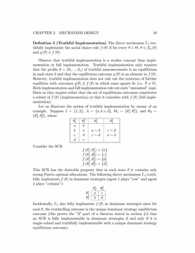
mentation or full implementation. Truthful implementation only requiresthat the profile θ = (θ1, ..., θn) of truthful announcements is an equilibriumin each state θ and that the equilibrium outcome g (θ) is an element in f (θ).However, truthful implementation does not rule out the existence of furtherequilibria with outcomes g(θ) /∈ f (θ) in which some agents lie (i.e. θ 6= θ).Both implementation and full implementation rule out such ”unwanted” equi-libria as they require either that the set of equilibrium outcomes constitutesa subset of f (θ) (implementation) or that it coincides with f (θ) (full imple-mentation).Let us illustrate the notion of truthful implementation by means of an

example. Suppose I = {1, 2}, A = {a, b, c, d}, Θ1 = {θ11, θ21}, and Θ2 ={θ12, θ22}, where

θ11 θ21 θ12 θ22abcd

badc

a ∼ bc ∼ d

c ∼ da ∼ b

Consider the SCRf (θ11, θ

12) = {a}

f (θ11, θ22) = {c}

f (θ21, θ12) = {b}

f (θ21, θ22) = {d}

This SCR has the desirable property that in each state θ it contains onlystrong Pareto optimal allocations. The following direct mechanism Γd truth-fully implements f (θ) in dominant strategies (agent 1 plays ”row” and agent2 plays ”column”):

θ12 θ22θ11 a cθ21 b d

Incidentally, Γd also fully implements f (θ) in dominant strategies since foreach θ, the truthtelling outcome is the unique dominant strategy equilibriumoutcome (this proves the ”if”-part of a theorem stated in section 2.2 thatan SCR is fully implementable in dominant strategies if and only if it issingle-valued and truthfully implementable with a unique dominant strategyequilibrium outcome).


2.2 Dominant Strategy ImplementationThe Revelation Principle

The great virtue of dominant strategy equilibrium is that agents need notforecast how other agents choose their strategies. In other words, agents donot have to know each others’ preferences. This is the basis for an extremelyconvenient result known as the revelation principle (Gibbard (1973), Greenand Laffont (1977), Dasgupta, Hammond, and Maskin (1979)), which saysthat we can restrict attention to direct mechanisms in which agents reportonly their own types. Thus, the assumption of complete information made atthe beginning of this chapter is irrelevant and any result derived in this sec-tion continues to hold if this assumption is dropped. Due to this robustnessproperty, SCRs that are truthfully implementable in dominant strategies areof particular interest.

Definition 6 (TIDS Social Choice Rule) The social choice rule f (θ) istruthfully implementable in dominant strategies (TIDS) or strategy-proof ifthere exists a direct mechanism Γd such that i) truthtelling is a dominantstrategy equilibrium, i.e. if for all i ∈ I and θi ∈ Θi,

g(θi, θ−i) %i (θi) g(θi, θ−i) (2.3)

for all θi ∈ Θi, θ−i ∈ Θ−i, and ii) g (θ) ∈ f (θ) for all θ ∈ Θ.We now present the revelation principle, which asserts that for every

mechanism Γ that implements f (θ) in dominant strategies, we can find adirect mechanism Γd that truthfully implements f (θ) in dominant strategies.

Theorem 1 (Revelation Principle) If an SCR is implementable in dom-inant strategies, then it is TIDS.

Proof (direct) Suppose Γ implements the social choice rule f (θ) in domi-nant strategies, and let Eg (θ) be non-empty for all θ. Define an equilibriumselection as a mapping s∗ : Θ → ×Si which selects exactly one equilibriumprofile s∗ (θ) ∈ Eg (θ) for each θ ∈ Θ. Since s∗ (θ) is a dominant strategyprofile, we have

g (s∗i (θi) , s−i) %i (θi) g (si, s−i) (2.4)

for all i ∈ I, θi ∈ Θi, si ∈ Si, and s−i ∈ S−i. In particular, it is true thatg(s∗i (θi) , s

∗−i(θ−i)) %i (θi) g(s∗i (θi), s∗−i(θ−i)) (2.5)

for all i ∈ I, θi, θi ∈ Θi and θ−i ∈ Θ−i since s∗i (θi) ∈ Si and s∗−i(θ−i) ∈ S−iare merely specific strategies.


Next, define the composed mapping h : Θ → A with h (θ) ≡ g (s∗ (θ)).The function h (θ) together with the collection of possible types {Θ1, ...,Θn}defines a direct mechanism Γd. But Γd truthfully implements f (θ) in domi-nant strategies because h (θ) ≡ g (s∗ (θ)) ∈ f (θ) and

h(θi, θ−i) %i (θi) h(θi, θ−i) (2.6)

for all i ∈ I, θi, θi ∈ Θi and θ−i ∈ Θ−i. Thus, f (θ) is TIDS.

Remarks

1. The intuition that underlies the proof is straightforward. For each stateθ, consider an equilibrium profile s∗ (θ) = (s∗1 (θ1) , ..., s

∗n (θn)) induced

by the (indirect) mechanism Γ with outcome g (s∗ (θ)) ∈ f (θ). Theplanner can mimick Γ by asking each agent to announce a type θi andplaying on his behalf the strategy s∗i (θi). Since s

∗i (θi) is a dominant

strategy in the game induced by Γ, reporting the true type θi = θimust also be a dominant strategy in the new game. Notice that wehave assumed that the planner can commit to playing s∗i (θi) after theagents have revealed their types.

2. Since full implementation implies implementation, theorem 1 continuesto hold if we substitute ”implementable” with ”fully implementable”.

3. In the remainder of this section, we will characterize the set of SCRsthat are implementable in dominant strategies. In theory, this impliesthat we have to consider all possible mechanisms. However, due to therevelation principle, we can restrict attention (subject to a caveat) todirect mechanisms and identify the set of SCRs that are TIDS.

4. Here is the caveat mentioned in 3. According to the revelation prin-ciple, TIDS is a necessary, but not a sufficient condition for dominantstrategy implementation. Hence, if an SCR is not TIDS, we can besure that it is not implementable in dominant strategies. However,the converse is not true, i.e. there may exist SCRs that are TIDS butnot implementable in dominant strategies. For instance, if truthtellingis only a weakly dominant strategy and there exist other (untruthful)equilibria in weakly dominant strategies with outcomes g(θ) /∈ f (θ),then the direct mechanism Γd does not implement f (θ), even thoughit truthfully implements f (θ). Conditions under which the revelationprinciple also holds in the other direction are presented in the followingsubsection.


Necessary and Sufficient Conditions for Implementation

Consider a direct mechanism Γd that truthfully implements f (θ) in dominantstrategies with a unique outcome in each state. Per definition, Γd implementsf (θ) in dominant strategies. Moreover, when f (θ) is single-valued, the con-cepts of implementation and full implementation coincide and Γd also fullyimplements f (θ) in dominant strategies. This suggests that the revelationprinciple holds in the other direction as well if we can ensure that the out-come associated with truthtelling is the unique dominant strategy equilibriumoutcome. A sufficient condition for a game to have at most one dominantstrategy outcome is that < contains only strict preference orderings.

Theorem 2 Suppose that < contains only strict preference orderings. If anSCR is TIDS, then it is implementable in dominant strategies.

Proof (direct) Assume that the direct mechanism Γd truthfully implementsf (θ) in dominant strategies. Since < contains only strict orderings, the setg (Eg (θ)) ≡ {g(θ) | θ ∈ Eg (θ)} of dominant strategy equilibrium outcomesmust be a singleton set for all θ ∈ Θ. Because the social choice rule f (θ)is TIDS, θ ∈ Eg (θ) and g(θ) ∈ f (θ). This implies g (Eg (θ)) ⊆ f (θ) for allθ ∈ Θ, i.e. f (θ) is implementable.

Theorem 2 shows that strict preference orderings and truthful implemen-tation imply implementation. The following theorem goes beyond theorem2 by showing that strict preference orderings, truthful implementation andsingle-valuedness of f (θ) imply full implementation. In addition, it showsthat the reverse also holds.

Theorem 3 Suppose that < contains only strict preference orderings. AnSCR is fully implementable in dominant strategies if and only if it is TIDSand single-valued.

Proof (direct) ”if”-part: By theorem 2, strict preference orderings andTIDS imply implementability. When the social choice rule f (θ) is single-valued, the concepts of implementability and full implementability coincide.It follows that f (θ) is fully implementable.”only if”-part: By Theorem 1, full implementability implies TIDS. More-

over, if < contains only strict preference orderings, the set of dominant strat-egy equilibrium outcomes g (Eg (θ)) ≡ {g (s∗ (θ)) | s∗ (θ) ∈ Eg (θ)} is a sin-gleton set for all θ ∈ Θ. Hence every fully implementable SCR must besingle-valued.


The Gibbard-Satterthwaite Theorem

In virtually all economic applications of interest, dictatorial SCRs are viewedas undesirable (recall that the social choice set f (θ) of a dictatorial SCRis a subset of the most preferred outcomes of a particular agent i in eachstate). For instance, democratic voting rules such as the majority rule aregenerically non-dictatorial. Also, the decision whether to provide a publicgood is typically not based on the valuation of a particular individual, butdepends on the valuations of all the agents in the economy. Likewise, auctionsdo typically not assign the object in question to a single predetermined agent,but to the bidder with the highest valuation.Given the prevalence of non-dictatorial SCRs, it is disturbing to learn that

under some very general conditions, none of these SCRs is implementable indominant strategies. In fact, the following theorem due to Gibbard (1973)and Satterthwaite (1975) tells us that when the domain of the agents’ pref-erence orderings is unrestricted, only dictatorial SCRs can be implementedin dominant strategies.

Definition 7 (Dictatorial Social Choice Rule) The social choice rulef (θ) is dictatorial on the set A0 ⊆ A if there exists an agent i ∈ I suchthat for all θ ∈ Θ, the choice set f (θ) is a subset of agent i’s most preferredoutcomes in A0, i.e. f (θ) ⊆ {y ∈ A0 | y %i (θi) z for all z ∈ A0}.

Theorem 4 (Gibbard-Satterthwaite Theorem) Let the social choicerule f (θ) be single-valued and let A0 ⊆ A denote the range of f (θ). Supposethat A is finite, that A0 contains at least three elements, and that for eachagent i ∈ I, the set of possible preference orderings <i is the set of strictpreference orderings on A. Then f (θ) is TIDS if and only if it is dictatorialon A0.

Proof The ”if”-part is obvious: Any dictatorial single-valued SCR is TIDS(assume that agent i is the dictator. In the direct mechanism Γd, we can thensimply assign an element in the set {y ∈ A0 | y %i (θi) z for all z ∈ A0} to anyprofile of announcements θ containing θi). The outline of the ”only if”-partis as follows: From f (θ), we construct a social welfare function (SWF ) F (θ)that is maximized by f (θ) and fulfills the conditions of Arrow’s impossibilitytheorem. It follows that F (θ) is dictatorial, which in turn implies that f (θ)is dictatorial.

The full proof of the ”only if”-part is lengthy and is omitted for the sakeof brevity. For a complete version of the proof, see Green and Laffont (1979),theorem 2.2.


Remarks

1. Some intuition for the Gibbard-Satterthwaite theorem can be gained bylooking at definition 6 which defines SCRs that are TIDS: In a simplesetting with two agents and two possible types per agent, TIDS impliesthat an SCR must satisfy 16 incentive compatibility constraints. Giventhese restrictive requirements, it is somewhat less surprising that onlydictatorial SCRs are TIDS.

2. In the face of this daunting result, we can choose between two possibil-ities: We can either relax the assumption of unrestricted preferences orwe can abandon the concept of dominant strategy implementation al-together. In the remainder of this section, we pursue the first approachand assume that preferences are restricted to the quasilinear domain.The second approach is pursued in sections 2.3 and 2.4 where we studyNash and Bayesian implementation, respectively.

Groves Mechanisms

In the remainder of this section, we concentrate on the special, but muchstudied problem introduced at the beginning of this chapter whether to pro-vide a public good. Consider the following additional assumptions:

9. A feasible outcome is a profile y = (x, t1, ..., tn) ∈ A consisting of adecision x ∈ {0, 1} and a vector of monetary transfers t = (t1, ..., tn).

10. The agents’ preferences are quasilinear of the form θix + ti. Here, thetype θi represents agent i’s valuation or willingness to pay for the publicgood.

In the public good context, x = 1 means that the public good is providedand x = 0 means that it is not provided. However, the same frameworkcan be used to represent an auction setting where an indivisible good isauctioned off to one of n agents. In this case, the decision x is a profilex = (x1, ..., xn), where xi = 1 means that agent i receives the good andxi = 0means that he does not receive the good (which imposes the additionalconstraint

Pi xi = 1). The agents’ preferences then take the form θixi + ti.

Without loss of generality, we can assume that the cost of the public goodis zero (if the cost is c ≥ 0, we simply let each agent pay an equal sharecnand redefine the agents’ valuations as θi = θi − c

n, where θi is now a net

valuation). Note that ti can be negative.When the agents’ utilities are cardinally and interpersonally comparable,

a reasonable social objective is the maximization of the utilitarian SWF


F (θ) =P

i (θix+ ti). The solution to this problem is x = 1 if and onlyifP

i θi ≥ 0, i.e. the public good is provided if and only if the sum ofthe agents’ valuations exceeds the cost of the public good c = 0. Let ushenceforth restrict attention to SCRs that meet this welfare criterion. SuchSCRs are called successful.

Definition 8 (Successful Social Choice Rule) The social choice rulef (θ) = (x (θ) , t1 (θ) , ..., tn (θ)) is successful if

x (θ) =

½1 if

Pi θi ≥ 0

0 otherwise.(2.7)

Since successful SCRs have such desirable welfare properties, we would like tofind out whether they are also TIDS. In what follows, we show that successfulSCRs are indeed truthfully implementable in dominant strategies by a classof direct mechanisms known as Groves mechanisms due to Groves (1973).

Definition 9 (Groves Mechanism) A Groves mechanism ΓG is a directmechanism with

x(θ) =

½1 if

Pi θi ≥ 0

0 otherwise,(2.8)

ti(θ) =

( Pj 6=i θj + hi(θ−i) if

Pi θi ≥ 0

hi(θ−i) otherwise,(2.9)

for all i ∈ I, where θ is a profile of announcements, and where hi(θ−i) is anarbitrary function of θ−i.

In a Groves mechanism, agent i’s transfer ti(θ) depends on his announce-ment θi only insofar as this announcement affects the decision x(θ), given theannouncements

Pj 6=i θj of the remaining j 6= i agents. If x(θ) is changed,

agent i’s transfer is reduced by an amount equal to the sum of the otheragents’ valuations |Pj 6=i θj |, which corresponds exactly to the negative ex-ternality that agent i is imposing on these agents. Since externalities arenow fully internalized, agent i no longer benefits from free riding at the ex-pense of the other agents by misreporting his type and truthtelling becomesa dominant strategy.

Theorem 5 In a Groves mechanism ΓG, truthtelling is a dominant strategy.

Proof (direct) Denote the true and the announced type of agent i by θiand θi, respectively, and denote the announcements of the other j 6= i agentsby θ−i.


i) Suppose that θi +P

j 6=i θj ≥ 0. Any announcement θi 6= θi such thatθi +

Pj 6=i θj ≥ 0 yields the same utility as truthtelling, viz. θi +

Pj 6=i θj +

hi(θ−i). Any announcement θi 6= θi such that θi+P

j 6=i θj < 0 yields hi(θ−i),which is less than or equal to θi +

Pj 6=i θj + hi(θ−i) since θi +

Pj 6=i θj ≥ 0.

Thus, agent i is never worse off by telling the truth.ii) Suppose now that θi +

Pj 6=i θj < 0. Any announcement θi 6= θi such

that θi+P

j 6=i θj < 0 yields the same utility as truthtelling, viz. hi(θ−i). Any

announcement θi 6= θi such that θi+P

j 6=i θj ≥ 0 yields θi+P

j 6=i θj+hi(θ−i),which is less than hi(θ−i) since θi+

Pj 6=i θj < 0. Again, agent i is never worse

off by telling the truth.

Since truthtelling is a dominant strategy, (2.7) and (2.8) coincide, fromwhich it follows that the Groves mechanism truthfully implements successfulSCRs in dominant strategies. Perhaps even more intriguing is the followingresult, which states that the Groves mechanism ΓG is the only mechanismthat truthfully implements successful SCRs in dominant strategies.

Theorem 6 Any mechanism Γd that truthfully implements a successful SCRin dominant strategies coincides with the Groves mechanism.

Proof (indirect) We prove the logically equivalent statement that anymechanism Γd that does not coincide with the Groves mechanism cannottruthfully implement a successful SCR in dominant strategies. From defi-nition 9, a mechanism Γd is a Groves mechanism if and only if it has thefollowing properties:i) x(θ) = 1 if and only if

Pi θi ≥ 0,

ii) Given θ−i, ti(θ) is constant for all i and θi such that θi +P

j 6=i θj ≥ 0,iii) Given θ−i, ti(θ) is constant for all i and θi such that θi+

Pj 6=i θj < 0,

iv) x(θi, θ−i) = 1 and x(θ0i, θ−i) = 0 imply ti(θi, θ−i)−ti(θ

0i, θ−i) =

Pj 6=i θj.

We now show that if Γd lacks one or more of these properties, then it eitherviolates success or TIDS or both. Since each property can either hold or fail,there are 24-1=15 possible events which contain at least one failure.1) Suppose property i) does not hold (8 cases). Then Γd either violates

success (if θ is the true state) or TIDS (if θ is not the true state).2) Assume that property i) holds but that property ii) fails (4 cases).

Then there exists an agent i and announcements θi (truthtelling), θi, and θ−isuch that θi +

Pj 6=i θj ≥ 0, θi +

Pj 6=i θj ≥ 0 (i.e. given θ−i, both θi and θi

yield x = 1) and t(θi, θ−i) > t(θi, θ−i). It follows that truthtelling is not adominant strategy for agent i.


3) Suppose properties i) and ii) hold but property iii) does not hold (2cases). Then there exists an agent i and announcements θi (truthtelling),θi, and θ−i such that θi +

Pj 6=i θj < 0, θi +

Pj 6=i θj < 0 (i.e. given θ−i,

both θi and θi yield x = 0) and t(θi, θ−i) > t(θi, θ−i). Again, it follows thattruthtelling is not a dominant strategy for agent i.4) Finally, assume that properties i), ii), and iii) hold and that prop-

erty iv) fails (1 case). Then x(θi, θ−i) = 1 and x(θ0i, θ−i) = 0 imply that

either a) ti(θi, θ−i) − ti(θ0i, θ−i) =P

j 6=i θj − ² or b) ti(θi, θ−i) − ti(θ0i, θ−i) =P

j 6=i θj + ² is true for some ² > 0 . Let us only consider the former pos-sibility (the proof of b) is along the same lines). If a) holds, then thereexists an agent i and announcements θi = θi (truthtelling), θ

0i, and θ−i such

that θ0i +

Pj 6=i θj < 0, θi = −Pj 6=i θj +

²2(hence θi +

Pj 6=i θj > 0) and

ti(θi, θ−i)− ti(θ0i, θ−i) =P

j 6=i θj − ². Agent i’s utility from telling the truth

is θi + ti(θi, θ−i) = ti(θ0i, θ−i) − ²

2, whereas his utility from announcing θ

0i is

ti(θ0i, θ−i) > ti(θ

0i, θ−i) − ²

2. It follows that truthtelling is not a dominant

strategy for agent i.

One implication of theorem 6 is that the only SCRs that are both success-ful and TIDS are those defined in (2.8)-(2.9). We can think of many exampleswhere we may want to place even further restrictions on the transfer functionti (θ). For instance, in some cases the planner may not be allowed to run adeficit when implementing f (θ), i.e. the sum

Pi ti (θ) must not exceed zero.

An SCR with this property is called feasible.

Definition 10 (Feasible Social Choice Rule) An SCR is feasible ifPi ti (θ) ≤ 0 for all θ ∈ Θ.

An even stronger requirement is that f (θ) be budget-balanced, i.e. thatthe sum of transfers

Pi ti (θ) be identically equal to zero.

Definition 11 (Budget-Balanced Social Choice Rule) An SCR is budg-et-balanced if

Pi ti (θ) = 0 for all θ ∈ Θ.

Since the planner’s preferences do not enter into our welfare considera-tions, any net surplus |Pi ti (θ)| > 0 collected from the agents is wasteful. Itis therefore not surprising that the social choice rule f ∗ (θ) which maximizesthe utilitarian SWF F (θ) =

Pi (θix+ ti) subject to the feasibility constraintP

i ti (θ) ≤ 0 is both successful and budget-balanced. Such an SCR is calledex-post efficient.


Definition 12 (Ex-Post Efficient Social Choice Rule) An SCR is ex-post efficient if it is both successful and budget-balanced.

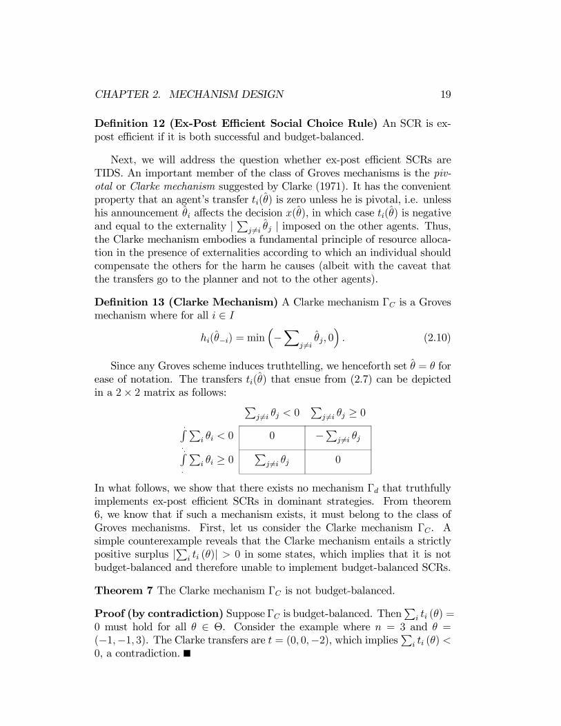
Next, we will address the question whether ex-post efficient SCRs areTIDS. An important member of the class of Groves mechanisms is the piv-otal or Clarke mechanism suggested by Clarke (1971). It has the convenientproperty that an agent’s transfer ti(θ) is zero unless he is pivotal, i.e. unlesshis announcement θi affects the decision x(θ), in which case ti(θ) is negativeand equal to the externality |Pj 6=i θj | imposed on the other agents. Thus,the Clarke mechanism embodies a fundamental principle of resource alloca-tion in the presence of externalities according to which an individual shouldcompensate the others for the harm he causes (albeit with the caveat thatthe transfers go to the planner and not to the other agents).

Definition 13 (Clarke Mechanism) A Clarke mechanism ΓC is a Grovesmechanism where for all i ∈ I

hi(θ−i) = min³−X

j 6=iθj, 0

´. (2.10)

Since any Groves scheme induces truthtelling, we henceforth set θ = θ forease of notation. The transfers ti(θ) that ensue from (2.7) can be depictedin a 2× 2 matrix as follows: P

j 6=i θj < 0P

j 6=i θj ≥ 0.R.

Pi θi < 0 0 −Pj 6=i θj

.R.

Pi θi ≥ 0

Pj 6=i θj 0

In what follows, we show that there exists no mechanism Γd that truthfullyimplements ex-post efficient SCRs in dominant strategies. From theorem6, we know that if such a mechanism exists, it must belong to the class ofGroves mechanisms. First, let us consider the Clarke mechanism ΓC. Asimple counterexample reveals that the Clarke mechanism entails a strictlypositive surplus |Pi ti (θ)| > 0 in some states, which implies that it is notbudget-balanced and therefore unable to implement budget-balanced SCRs.

Theorem 7 The Clarke mechanism ΓC is not budget-balanced.

Proof (by contradiction) Suppose ΓC is budget-balanced. ThenP

i ti (θ) =0 must hold for all θ ∈ Θ. Consider the example where n = 3 and θ =(−1,−1, 3). The Clarke transfers are t = (0, 0,−2), which impliesPi ti (θ) <0, a contradiction.


Next, we prove that there is no other feasible mechanism in the class ofGroves mechanisms whose surplus dominates that of the Clarke mechanism.

Theorem 8 There exists no feasible Groves mechanism ΓG with |P

i ti (θ)| ≤|Pi ti (θ)| for all θ ∈ Θ and |Pi ti (θ)| < |Pi ti (θ)| for some θ ∈ Θ, whereti (θ) denotes the Clarke transfer to agent i.

The proof is lengthy and is omitted here. See Laffont and Maskin (1982),theorem 3.3. for a complete proof.Theorems 7 and 8 together imply that no budget-balanced Groves mech-

anism exists. But by theorem 6, Groves mechanisms are the only candidatesfor truthful implementation of ex-post efficient SCRs. This leads to the fol-lowing trivial, but important corollary:

Corollary 1 There exists no SCR that is both TIDS and ex-post efficient.

Remarks

1. While there is no SCR that is both ex-post efficient and TIDS, theredo exist SCRs which are successful, feasible, and TIDS. In fact, anySCR that is implemented by the Clarke mechanism has this property.

2. More encouraging results can be obtained when the underlying equi-librium concept is weakened so that less incentive compatibility con-straints must be satisfied. For instance, in sections 2.3 and 2.4 wewill show that ex-post efficient SCRs are implementable in Nash andBayesian equilibrium, respectively.

3. At the beginning of this subsection, we pointed out the analogy be-tween the public good model and a setting where an indivisible good isauctioned off to one of n agents. In the auction setting, the analogue ofthe Clarke mechanism is known as second-price sealed-bid or Vickreyauction. There, agent i is pivotal if he is the bidder with the highestvaluation, and his transfer ti(θ) is equal to the second-highest valuationmax{θj | j 6= i}, which is again the externality caused by agent i.

4. Despite the striking similarity, the public good setting and the auc-tion setting differ in an important aspect: In the auction setting, theplanner coincides with the seller, whose utility enters into our welfareconsiderations. An immediate consequence of this is that the SCR im-plemented by the Clarke-Vickrey mechanism is then ex-post efficientsince the surplus |Pi ti (θ)| > 0 collected by the planner (”agent 0”) isno longer wasteful. More generally, any profile of transfers is compati-ble with a Pareto optimal allocation.


Finally, we look at situations where the planner cannot force the agentsto take part in the game. When participation is voluntary, an implementableSCR must satisfy an additional set of constraints known as individual ratio-nality or participation constraints. These constraints ensure that each agentcan guarantee himself a certain minimum utility (typically normalized tozero) by telling the truth.

Definition 14 (Ex-Post Individually Rational Social Choice Rule)An SCR is ex-post individually rational if θix (θ)+ t (θ)i ≥ 0 for all i ∈ I andθ ∈ Θ.

In the absence of voluntary participation, it was shown that successfuland feasible SCRs can be truthfully implemented in dominant strategies.When individual rationality constraints are added, this turns out impossible.

Theorem 9 There exists no SCR that is TIDS, successful, feasible, andex-post individually rational.

Proof (by contradiction) Suppose there exist SCRs that are TIDS, suc-cessful, feasible, and ex-post individually rational. By theorems 6 and 5, wecan restrict attention to Groves mechanisms. Choose a profile θ = (θ1, ..., θn)such that

Pi θi ≥ 0 and such that for all i ∈ I, there exists a θ0i with

θ0i +P

j 6=i θj < 0. Given that the other agents are of type θ−i, the func-tion hi (θ−i) to agent i is the same for type θi or type θ0i. If agent i is oftype θ0i, success implies x = 0. From individual rationality, it then followsthat hi (θ−i) ≥ 0. This is true for all i ∈ I. Consider now the case whereθ = (θ1, ..., θn). Success implies x = 1, and feasibility requiresX

i

ti =Xi

Xj 6=iθj +

Xi

hi (θ−i) = (n− 1)Xi

θi +Xi

hi (θ−i) ≤ 0. (2.11)

SinceP

i θi ≥ 0, this impliesP

i hi (θ−i) < 0, a contradiction.

2.3 Nash ImplementationDirect vs. Indirect Mechanisms

The previous section made clear that very little is implementable in domi-nant strategies: For unrestricted preference domains, it was shown that onlydictatorial SCRs are TIDS, and when preferences were restricted to the qua-silinear domain, it was shown that no SCR is both ex-post efficient and TIDS.A less restrictive equilibrium concept than dominant strategy equilibrium is


Nash equilibrium. For a strategy s∗i to be an equilibrium strategy, it needonly be optimal with respect to the other players’ equilibrium strategies s∗−i,as opposed to dominant strategy equilibrium, where s∗i must be optimal withrespect to any profile s−i in the other players’ strategy set ×S−i.In section 2.2, it turned out to be convenient to restrict attention to direct

mechanisms and concentrate on SCRs that are truthfully implementable.

Definition 15 (TINS Social Choice Rule) The social choice rule f (θ)is truthfully implementable in Nash strategies (TINS) if there exists a directmechanism Γd such that i) truthtelling is a Nash equilibrium, i.e. if for alli ∈ I, θi ∈ Θi, and θ−i ∈ Θ−i,

g(θi, θ−i) %i (θi) g(θi, θ−i) (2.12)

for all θi ∈ Θi, and ii) g (θ) ∈ f (θ) for all θ ∈ Θ.We could now proceed by deriving a corresponding version of theorem

1 (revelation principle) for Nash implementation. Unfortunately, restrictingattention to direct mechanisms does not get us any further since the set ofSCRs that are TINS is no greater than the set of SCRs that are TIDS, whichbrings us back to dominant strategy implementation.

Theorem 10 An SCR is TINS if and only if it is TIDS.

Proof (direct) The ”if”-part is obvious, since any dominant strategy equi-librium is a Nash equilibrium.”Only if”-part: Assume that the direct mechanism Γd truthfully imple-

ments f (θ) in Nash strategies. Then for all i and θi, θi, and θ−i ∈ Θ−i,g(θi, θ−i) %i (θi) g(θi, θ−i), from which it follows that truthtelling is a domi-nant strategy.

The ”only if”-part is nothing but a restatement of definition 15. There,we required that θi is optimal with respect to any possible profile θ−i inthe other players’ strategy set Θ−i, which coincides with the definition of adominant strategy. Alternatively, by setting θ−i = θ−i, we see that definitions15 and 6 are equivalent. Intuitively, remember that the direct mechanism Γdinduces a game of complete information in every state θ. In any such game,TINS requires only that announcing θi is optimal with respect to the profileof true announcements θ−i. Thus, fix θi and consider the states (θi,θ−i),(θi,θ0−i), (θi,θ

00−i) etc. such that {θ−i, θ0−i, θ00−i, ...} = Θ−i. Clearly, requiring

that θi is optimal with respect to any possible profile of truthful reportsθ−i, θ0−i, θ

00−i, ... ∈ Θ−i amounts to the same as requiring that θi is a dominant

strategy.


The reasoning which underlies theorem 10 does not apply if we define astrategy set in Γd as the entire state spaceΘ = ×Θi. That is, instead of havingagents announce their types θi, we let each agent announce a complete profileθ = (θ1, ..., θn). In this case, SCRs that are TINS are no longer automaticallyTIDS, and we can hope that by restricting attention to direct mechanisms,more SCRs are truthfully implementable in Nash strategies than in dominantstrategies. Unfortunately, it turns out that with this enlarged definition ofstrategy sets, any SCR is TINS. To see this, let the true state be θ andconsider the direct mechanism Γd which implements outcome y ∈ f(θ) ifand only if all agents announce the same θ. If one or more agents disagree,a ”bad” outcome is implemented (e.g. all agents are shot). Clearly, thismechanism has θ = θ as a Nash equilibrium and thus truthfully implementsf(θ). But any common report θ 6= θ is also a Nash equilibrium, from whichit follows that f(θ) is not implemented unless all equilibria have outcomesthat are in f(θ).Although there exists a version of the revelation principle for Nash imple-

mentation (cf. Repullo (1986), theorem 6.1), it is of little use here becauserestricting attention to direct mechanisms implies a great loss of generalitydue to the multiple equilibrium problem. In the remainder of this section,we therefore focus on indirect mechanisms.

Necessary and Sufficient Conditions for Implementation

Consider a social choice rule f(θ) that is implementable in Nash strategiesand select a particular state θ0. This state has at least one Nash equilibriumwhose outcome, say y, is in f(θ0). Next, select a different state θ00 andassume that y (weakly) moves up everyone’s ranking when switching fromθ0 to θ00. Clearly, the Nash equilibrium with outcome y continues to be aNash equilibrium in state θ00. By the definition of implementability, y musttherefore also be an element of f(θ00). An SCR with the property that anoutcome y that is an element of f(θ0) and does not fall in anyone’s rankingwhen moving from θ0 to θ00 is also an element of f(θ00) is called monotonic.By the above reasoning, any Nash implementable SCR must be monotonic.

Definition 16 (Monotonic Social Choice Rule) The social choice rulef(θ) is monotonic if for all y ∈ A and θ0, θ00 ∈ Θ, the following holds: if i)y ∈ f(θ0) and ii) for all i ∈ I and z ∈ A, y %i (θ0) z ⇒ y %i (θ00) z, theny ∈ f(θ00).

An immediate consequence of definition 16 is the following property ofmonotonic SCRs: If y ∈ f (θ0) and y /∈ f (θ00), then there exists at least one


agent i and outcome z such that y %i (θ0i)z and z Âi (θ00i )y. Let us henceforthcall z a test outcome with respect to (y, θ0, θ00) and the agent i for whom thispreference reversal holds a test agent with respect to (y, θ0, θ00).The assertion that Nash implementability implies monotonicity is part of

a theorem due to Maskin (1977), which is considered as the most importantresult in the theory of Nash implementation.

Theorem 11 (Maskin’s Theorem I: Necessity) If an SCR is imple-mentable in Nash strategies, then it is monotonic.

Proof (by contradiction) If f(θ) is implementable in Nash strategies, thereexists a state θ0 ∈ Θ and a Nash equilibrium profile s∗ (θ0) = (s∗i (θ0) , s∗−i (θ0))with g (s∗ (θ0)) ∈ f(θ0). By the definition of Nash equilibrium,

g(s∗i (θ0) , s∗−i (θ

0)) %i (θ0i) g(si, s∗−i (θ0)) (2.13)

for all i ∈ I and si ∈ Si. Suppose now that f (θ) is not monotonic. Thenthere exists a state θ00 6= θ0 such that

g(s∗i (θ0) , s∗−i (θ

0)) %i (θ00i ) g(si, s∗−i (θ0)) (2.14)

for all i ∈ I and si ∈ Si but g (s∗ (θ0)) /∈ f (θ00). However, from (2.14)it follows that the profile s∗ (θ0) with outcome g (s∗ (θ0)) continues to be aNash equilibrium in state θ00, which contradicts the assumption that f(θ) isimplementable.

Remarks

1. Since full implementation implies implementation, theorem 11 con-tinues to hold if we substitute ”implementable” with ”fully imple-mentable”.

2. For the case of single-valued SCRs, it can be shown that an SCR is im-plementable in Nash strategies only if it is truthfully implementable indominant strategies (given that the domain of preferences is monoton-ically closed - a property that we will not define here). Thus, nothingis gained from weakening the underlying equilibrium concept. Evenworse, under some fairly innocuous assumptions, a result reminiscentof the Gibbard-Satterthwaite theorem can be proven which says thatan SCR is implementable in Nash strategies if and only if it is dictator-ial. For a proof, see Dasgupta, Hammond, and Maskin (1979), theorem7.2.3. and corollary 7.2.5.


3. Monotonicity is satisfied by such common SCRs as the Paretian choicerule and the majority rule (if < consists of strict orderings). Further-more, monotonicity is closely related to Arrow’s well-known ”indepen-dence of irrelevant alternatives” condition. For instance, suppose thatby switching from state θ0 to state θ00, the set L (y) of outcomes thatall agents value less than y remains the same (L (y) is called the lowercontour set with respect to y), but that the relative rank order of someof the elements in L (y) changes for some agents. Then, monotonicityrequires that if y is in f (θ0), it must also be in f (θ00), regardless of thechanges in L (y).

4. Monotonicity rules out interpersonal comparisons of the kind inherentin utilitarian or Rawlsian SCRs: The only thing that matters whenswitching from state θ0 to θ00 is that no agent values y less than before.Whether some agents value y much higher while others value y onlyslightly higher is inconsequential.

The second part of Maskin’s theorem shows that monotonicity togetherwith the additional condition of no veto power implies full implementability.

Definition 17 (No Veto Power) The social choice rule f (θ) satisfies noveto power if for all i ∈ I and y ∈ A, the following holds: if for all j 6= i andz ∈ A, y %j (θj) z, then y ∈ f (θ).

In words, no veto power says that whenever in some state θ an outcomey is top-ranked for n− 1 agents, then y should be in the choice set f (θ), i.e.the remaining agent cannot veto it.

Theorem 12 (Maskin’s Theorem II: Sufficiency) Suppose n ≥ 3. If anSCR is monotonic and satisfies no veto power, then it is fully implementablein Nash strategies.

Proof (by contradiction) Consider the following mechanism: Each agentannounces a state, an outcome, and a nonnegative integer.i) If all agents agree on some state θ and outcome y ∈ f (θ), then y is

implemented.ii) If n− 1 agents agree on some state θ and outcome y ∈ f (θ), then y is

implemented unless the remaining agent i announces a state θ0 and outcomez such that I) y /∈ f (θ0), II) i is a test agent for (y, θ, θ0), and III) z is a testoutcome for (y, θ, θ0), in which case z is implemented.iii) In all other cases, the outcome of the agent with the highest integer

is implemented.


First, we show that if the true state is θ, there exists a Nash equilibriumfor each y ∈ f (θ) where all agents announce (y, θ). Suppose that this isnot the case. Then there must exist an agent i who strictly benefits fromannouncing a pair (z, θ0) that satisfies conditions I)-III) (any other unilateraldeviation leads to y being implemented and thus cannot be strictly prof-itable). By definition, i is a test agent and z is a test outcome for (y, θ, θ0),from which it follows that y %i (θi) z. However, strict profitability impliesthat z Âi (θi) y, a contradiction.Next, we show that if the true state is θ, no Nash equilibrium with out-

come z /∈ f (θ) exists. Suppose that such an equilibrium exists. From i)-iii),we conclude that this Nash equilibrium must belong to one of the followingtwo categories:1) All agents agree on some state θ0 and outcome z, where z ∈ f (θ0)

and z /∈ f (θ). By monotonicity, there exists a test outcome y and a testagent i who strictly prefers to unilaterally deviate by announcing (y, θ) acontradiction.2) n−1 agents agree on some state and outcome and the remaining agent

disagrees. Denote the outcome from this equilibrium by z /∈ f (θ). Thereare two possibilities: a) There exists an x ∈ A such that one of the n − 1agents strictly prefers x to z. This agent is strictly better off by unilaterallydeviating from the proposed equilibrium, a contradiction (he will announce adifferent state, together with x and some integer that exceeds the integers ofthe other agents). b) z is top-ranked for all n− 1 agents. By no veto power,z ∈ f (θ), which contradicts the assumption that z /∈ f (θ).Remarks

1. The role of the integers is solely to rule out Nash equilibria based onstep iii) of the mechanism with unwanted outcomes z /∈ f (θ). Sincethe set of integers is unbounded, such equilibria cannot exist. For anyprofile of integers announced by the remaining j 6= i agents, agent iwould always want to deviate by announcing a higher integer.

2. The assumption of no veto power is trivially satisfied in any examplewith n ≥ 3 agents in which there is a private good that yields positiveutility (e.g. money). Because each agent wants to have all of the privategood himself, there cannot exist situations in which n− 1 agents agreeon the same outcome. Then, monotonicity constitutes both a necessaryand sufficient condition for full Nash implementability.

3. When n = 2, a result similar to theorem 12 can be proven if in addi-tion to monotonicity, f (θ) satisfies a condition called restricted no vetopower. See Moore and Repullo (1990), corollary 3, for details.


The Public Good Problem Revisited

In section 2.2, we saw that even if preferences are restricted to the quasi-linear domain, ex-post efficient SCRs cannot be implemented in dominantstrategies. We now reconsider the public good problem studied earlier andshow that with Nash implementation, life is much easier.First, note that no veto power is trivially satisfied in the public good

setting since preferences depend positively on the monetary transfers ti. Itthen follows from Maskin’s theorem that an SCR is fully implementable inNash strategies if and only if it is monotonic. We can now apply definition16 to the present context and conclude that an SCR is monotonic iff

(0, t1, ..., tn) ∈ f (θ) and θ ≥ θ0 implies (0, t1, ..., tn) ∈ f (θ0) , (2.15)

(1, t1, ..., tn) ∈ f (θ) and θ ≤ θ0 implies (1, t1, ..., tn) ∈ f (θ0) . (2.16)

In words: If an outcome y in the choice set implies x = 0 and the profile ofvaluations θ = (θ1, ..., θn) decreases in the vector sense, then y should remainin the choice set. Conversely, if an element in the choice set implies x = 1and the profile θ increases in the vector sense, then y should remain in thechoice set. Notice that a decrease in θ implies an increase in each agent’svaluation for outcomes that contain x = 0.Conditions (2.15)-(2.16) reveal that monotonicity places only very little

restriction on the vector of transfers (t1, ..., tn). In particular, the followingex-post efficient SCR is monotonic and therefore Nash implementable:

x(θ) =

½1 if

Pi θi ≥ 0

0 otherwise,(2.17)

ti(θ) = 0 for all i ∈ I. (2.18)

2.4 Bayesian ImplementationThe Revelation Principle

We now turn to environments where agents cannot observe each others’ pref-erences. As was remarked earlier, agents who possess a dominant strategywill use it even if they do not have complete information about the otheragents’ types. One implication of this is that the results derived in connec-tion with dominant strategy implementation continue to hold in the presenceof incomplete information. In this section, we employ the weaker concept ofBayesian (Nash) equilibrium. Consider the following assumptions which re-place assumption 5 of the basic model:


5a. Each agent observes only his own type θi, i.e. agents have incompleteinformation.

5b. The profile of types θ = (θ1, ..., θn) is drawn from the set Θ = ×Θiaccording to the distribution function Π (θ) with density π (θ), whichis common knowledge.

5c. The agents’ types are statistically independent, i.e. π (θ) =Qi∈I πi (θi).

The assumption of common knowledge in 5b is important and knownin game theory as common prior assumption or Harsanyi doctrine. It iscrucial, because in a game of incomplete information a player’s strategy notonly depends on his beliefs about π (θ), but also on his beliefs about others’beliefs about π (θ), beliefs about beliefs about beliefs, etc.If assumption 5c fails and types are correlated, a ”shoot-them-all” mech-

anism along the lines of that presented in section 2.2 can be used to truth-fully implement any social choice rule f (θ) as if information was complete.However, as was also shown in section 2.2, any common report is then anequilibrium and we are very far from actually implementing f (θ).In environments with incomplete information, a mechanism Γ combined

with the state-space Θ and density π (θ) defines a game of incomplete infor-mation with a (possibly) different payoff structure for every θ ∈ Θ. Fromnow on, let ui (y, θi) denote agent i’s von Neumann-Morgenstern utility overoutcomes when he is of type θi. As in the previous sections, we are especiallyinterested in SCRs that are truthfully implementable.

Definition 18 (TIBS Social Choice Rule) The social choice rule f (θ)is truthfully implementable in Bayesian strategies (TIBS) if there exists adirect mechanism Γd such that i) truthtelling is a Bayesian equilibrium, i.e.if for all i ∈ I and θi ∈ Θi,Z

Θ−iui (g(θi, θ−i), θi) dΠ−i (θ−i) ≥

ZΘ−iui(g(θi, θ−i), θi)dΠ−i (θ−i) (2.19)

for all θi ∈ Θi, and ii) g (θ) ∈ f (θ) for all θ ∈ Θ.According to (2.19), truthtelling need only be optimal in expected terms,

which is a weaker requirement than both TIDS (where θi = θi is to be optimalfor any profile θ−i) and TINS (where θi = θi is to be optimal for any profileof truthful reports θ−i).If the density function π (θ) is degenerate (i.e. if it has point mass only

on a single vector θ), Bayesian equilibrium reduces to ordinary Nash equilib-rium. Therefore, if we require that an SCR is implementable for all densities


(including degenerate ones), we inevitably run into the problems associatedwith Nash implementation. In particular, there is no point in restrictingattention to direct mechanisms as was shown in theorem 10.

Theorem 13 An SCR is TIBS for all possible densities π (θ) if and only ifit is TIDS.

Proof (indirect) The ”if”-part is obvious, since any dominant strategyequilibrium is a Bayesian equilibrium.”Only if”-part: Suppose f (θ) is not truthfully implementable in domi-

nant strategies. Then there exists an i ∈ I and a θ0 ∈ Θ such that truthtellingis not a Nash equilibrium strategy for agent i, given the profile of truthfulannouncements θ0−i. Now let π (θ

0) = 1. Then truthtelling is not a Bayesianequilibrium strategy either.

In the remainder of this section, we confine ourselves to density functionsπ (θ) which are not degenerate. Analogous to theorem 1, we can now derivea version of the revelation principle for Bayesian equilibrium.

Theorem 14 (Revelation Principle) If an SCR is implementable in Baye-sian strategies, then it is TIBS.

Proof (direct) Suppose that Γ implements the social choice rule f (θ) inBayesian strategies, and let Eg (θ) be non-empty for all θ. As in the proof oftheorem 1, s∗ : Θ→ ×Si is a mapping which selects exactly one equilibriumprofile s∗ (θ) ∈ Eg (θ) for each θ ∈ Θ. Since s∗ (θ) is a profile of Bayesianequilibrium strategies, we haveZ

Θ−iui¡g(s∗i (θi) , s

∗−i (θ−i)), θi

¢dΠ−i (θ−i) (2.20)

≥ZΘ−iui¡g(si, s

∗−i (θ−i)), θi

¢dΠ−i (θ−i)

for all i ∈ I, θi ∈ Θi, and si ∈ Si. In particular, it is true thatZΘ−iui¡g(s∗i (θi) , s

∗−i (θ−i)), θi

¢dΠ−i (θ−i) (2.21)

≥ZΘ−iui(g(s

∗i (θi), s

∗−i (θ−i)), θi)dΠ−i (θ−i)

for all i ∈ I and θi, θi ∈ Θi, since s∗i (θi) ∈ Si is merely a specific strategyrule.


Next, define the composed mapping h : Θ → A with h (θ) ≡ g (s∗ (θ)).The function h (θ) together with the collection of possible types {Θ1, ...,Θn}constitutes a direct mechanism Γd. But Γd truthfully implements f (θ) inBayesian strategies because h (θ) ≡ g (s∗ (θ)) ∈ f (θ) andZ

Θ−iui (h (θi, θ−i) , θi) dΠ−i (θ−i) ≥

ZΘ−iui(h(θi, θ−i), θi)dΠ−i (θ−i) (2.22)

for all i ∈ I and θi, θi ∈ Θi. It follows that f (θ) is TIBS.

Remarks

1. The revelation principle for Bayesian equilibrium is based on the sameintuition as the revelation principle for dominant strategy equilibrium.We therefore refer to the remarks made subsequent to theorem 1.

2. Contrary to an assertion by Laffont and Maskin (1982), p.44, the set ofBayesian equilibria in any indirect mechanism Γ is not isomorphic tothat in a corresponding direct mechanism Γd (cf. Repullo (1986), p.185for a counterexample). Hence, even if Γ gives rise to a unique Bayesianequilibrium, truthtelling may not be the unique equilibrium in Γd andrestricting attention to direct mechanisms leads to a loss of generality.

3. If it can be ensured that the truthtelling outcome is the sole equilibriumoutcome in the direct mechanism Γd, then the reverse of theorem 14is also true. Sufficient conditions for uniqueness are given by Repullo(1986), section 5, and Palfrey (1992), theorem 1.

By definition 18, TIBS imposes fewer incentive constraints than TIDS,which suggests that a wider range of SCRs is implementable in Bayesianstrategies than in dominant strategies. We will now show for the quasilinearframework that this is indeed true.

AGV Mechanisms

Let us return to the public good problem analyzed in section 2.2. There,we concluded that ex-post efficient SCRs are not implementable in dominantstrategies. For environments with complete information, we then showedthat this problem can be resolved by employing the weaker notion of Nashequilibrium. As it turns out, a similar result also holds in environments whereinformation is incomplete, i.e. there exists a mechanism that (truthfully)implements ex-post efficient SCRs. The mechanism in question in known


as AGV mechanism and was independently discovered by d’Aspremont andGérard-Varet (1979) and Arrow (1979).

Definition 19 (AGV Mechanism) An AGV mechanism ΓAGV is a directmechanism with

x(θ) =

½1 if

Pi θi ≥ 0

0 otherwise,(2.23)

ti(θ) =

ZΘ−i

³Xj 6=iθjx

³θi, θ−i

´´dΠ−i (θ−i) + hi(θ−i), (2.24)

where

hi(θ−i) = − 1

n− 1X

j 6=i

ZΘ−j

³Xk 6=j θkx

³θj, θ−j

´´dΠ−i (θ−j) (2.25)

for all i ∈ I, and where θ is a profile of announcements.

The logic which underlies the AGV mechanism is very similar to that ofthe Groves mechanism: Agent i’s transfer ti(θ) depends on his announcementθi only insofar as this announcement changes the decision x(θ), given that allother agents tell the truth. For any given profile of truthful announcementsθ−i, such a change in x(θ) reduces agent i’s transfer by an amount equalto the other agents’ valuations | Pj 6=i θj |, which represents the negativeexternality that he is imposing on these agents. Thus, the integral in (2.24)constitutes the expected (negative) externality from agent i’s announcement.Since all externalities are now fully internalized, no agent has an incentive tomisreport his type.

Theorem 15 In the AGV mechanism ΓAGV , truthtelling is a Bayesian equi-librium.

Proof (direct) Given that the remaining j 6= i agents tell the truth, agenti solves

maxθi

ZΘ−i(θix(θi, θ−i) + ti(θi, θ−i))dΠ−i (θ−i) . (2.26)

Because hi(θ−i) is independent of θi, this is equivalent to

maxθi

ZΘ−i

³θi +

Xj 6=iθj

´x(θi, θ−i)dΠ−i (θ−i) . (2.27)

By (2.23), θi = θi maximizes the integrand in (2.27) for any profile θ−i, whichimplies that θi = θi also maximizes the integral.


From theorem 15, it follows that an SCR with decision rule and trans-fer functions given by (2.23)-(2.24) is truthfully implementable in Bayesianstrategies. It is now a straightforward exercise to show that any such SCRis ex-post efficient.

Theorem 16 There exist SCRs that are both TIBS and ex-post efficient.

Proof (direct) Consider the social choice rule f (θ) with decision rule x (θ)and transfer functions ti (θ) given by (2.23)-(2.24). Success is obvious. Fur-thermore, by theorem 15, f (θ) is TIBS. In order to prove that it is alsobudget-balanced, let us define

τi(θi) ≡ZΘ−i

³Xj 6=iθjx

³θi, θ−i

´´dΠ−i (θ−i) . (2.28)

Since f (θ) is TIBS, we can set θi = θi. Summing over all i yieldsXiti (θ) =

Xiτi (θi)− 1

n− 1X

i

Xj 6=iτj (θj) (2.29)

=X

iτi (θi)− n− 1

n− 1X

iτi (θi)

= 0

for all θ ∈ Θ.

Hitherto, we have assumed that participation in the AGV mechanismis voluntary. If this assumption is relaxed, it may no longer be true thatΓAGV truthfully implements ex-post efficient SCRs in Bayesian strategies. Infact, as we will show later in the context of a bilateral trade problem, thereis no direct mechanism which truthfully implements ex-post efficient SCRsin Bayesian strategies and satisfies individual rationality at the same time.Prior to that, however, we characterize for a rather general class of problemsthe set of SCRs that are both TIBS and individually rational.

Necessary and Sufficient Conditions for Truthful Implementationwith Individual Rationality Constraints

For convenience, we maintain the assumption that preferences are quasilinear,albeit we consider now the more general form θivi (x) + ti, where x ∈ X ⊆Rk. In addition, let us replace assumption 3 of the basic model with

3a. Each agent has a characteristic or type θi ∈ Θi =£θi, θi

¤with θi 6= θi

and strictly positive density πi (θi) > 0 for all θi ∈ Θi.


For ease of exposition, let vi(θi) ≡RΘ−ivi(x(θi, θ−i))dΠ−i (θ−i) and ti(θi) ≡R

Θ−iti(θi, θ−i)dΠ−i (θ−i) denote agent i’s expected net benefit and expected

transfer, respectively, when he announces θi and the remaining j 6= i agentstell the truth. This allows us to write agent i’s expected utility from theprofile (θi, θ−i) as θivi(θi) + ti(θi). Finally, let Ui(θi) ≡ θivi(θi) + ti(θi) de-note agent i’s expected utility if everyone (including him) reveals his typetruthfully.The ex-post version of individual rationality given in definition 14 appears

overly strong for environments where information is incomplete. If we requirethat θivi (x (θ)) + t (θ)i ≥ 0 for all i ∈ I and θ ∈ Θ, then we essentially allowagents to withdraw from the game after everybody (truthfully) announcedhis type. It seems therefore more appropriate to require that an SCR beinterim individually rational in the sense that agents can only withdraw ata stage where they do not yet know each others’ types.

Definition 20 (Interim Individually Rational Social Choice Rule)An SCR is interim individually rational (IIR) if Ui (θi) ≥ 0 for all i ∈ I andθi ∈ Θi.

As in definition 14, the agents’ reservation utilities are normalized to zero.We can now characterize the set of SCRs that are both TIBS and IIR.

Theorem 17 An SCR is both TIBS and IIR if and only if for all i ∈ I,1) vi(θi) is nondecreasing,

2) Ui (θi) = Ui (θi) +R θiθivi(η)dη for all θi, and

3) Ui (θi) ≥ 0.

Proof (direct/by contradiction) ”if”-part: First, we show that 1) and 2)imply TIBS. Take any two values θi, θ0i ∈

£θi, θi

¤with θi > θ0i > θi. From 2),

we have

Ui (θi)−Z θi

θi

vi(η)dη = Ui(θ0i)−

Z θ0i

θi

vi(η)dη. (2.30)

Rearranging terms and using 1) gives

Ui (θi)− Ui(θ0i) =Z θi

θ0i

vi(η)dη ≥Z θi

θ0i

vi(θ0i)dη = (θi − θ0i)vi(θ0i). (2.31)

Note that vi(θ0i) is a constant. Hence

Ui (θi) ≥ Ui(θ0i) + (θi − θ0i)vi(θ0i) ≡ θivi(θ0i) + ti(θ0i). (2.32)


Similarly, suppose that θ0i > θi > θi. By the same reasoning, we have

Ui(θ0i) ≥ Ui(θi) + (θ0i − θi)vi(θi) ≡ θ0ivi(θi) + ti(θi). (2.33)

Together, (2.32) and (2.33) imply TIBS. Next, we prove that 1), 2), and 3)imply IIR. Suppose not. Then there exists some θi > θi with Ui (θi) < 0. Wejust established that 1) and 2) imply TIBS. However, TIBS in conjunctionwith 3) implies

Ui (θi) ≥ θivi(θi) + ti(θi) > θivi(θi) + ti(θi) ≡ Ui(θi) ≥ 0, (2.34)

a contradiction.”only if”-part: We now show that TIBS implies 1) and 2). For any i ∈ I

and any two types θi, θ0i ∈£θi, θi

¤, TIBS requires that

Ui (θi) ≥ θivi(θ0i) + ti(θ0i) ≡ Ui(θ0i) + (θi − θ0i)vi(θ0i), (2.35)

andUi(θ

0i) ≥ θ0ivi(θi) + ti(θi) ≡ Ui(θi)− (θi − θ0i)vi(θi). (2.36)

Suppose without loss of generality that θi < θ0i. From (2.35) and (2.36), itfollows that

vi(θ0i) ≥

Ui (θi)− Ui(θ0i)θi − θ0i

≥ vi(θi), (2.37)

which shows that vi(·) is nondecreasing. Next, letting θ0i → θi, we obtaindUi(θi)dθi

= vi(θi) for all θi. Integrating both sides over [θi, θi] gives

Ui (θi) = Ui (θi) +

Z θi

θi

vi(η)dη. (2.38)

for all θi Finally, note that IIR obviously implies 3) by definition 20.

Remarks

1. Theorem 17 is an extremely powerful tool in Bayesian implementationtheory and will be used repeatedly in the remainder of this section.An analogous version for the one-agent case was developed by Mirrlees(1971) and plays a central role in our analysis of adverse selection inchapter 3.

2. The great merit of theorem 17 is that it allows us to replace the origi-nal TIBS and IIR constraints with the mathematically more tractableconstraints 1)-3). Furthermore, direct inspection of conditions 1)-3)already yields many important insights as is shown in the followingsubsections in the context of a bilateral trading problem and auctiondesign.


The Myerson-Satterthwaite Theorem

Consider a bilateral trading problem where agent 1 is the seller of an indivisi-ble object that agent 2 likes to buy. Each agent has quasilinear utility θixi+ti,where θi and ti denote agent i’s valuation and transfer, respectively, andwhere xi is the probability that agent i receives the object. This setting corre-sponds in the framework of the previous subsection to the case where vi (x) =xi, and where X = {(x1, x2) | xi ∈ [0, 1] for i = 1, 2 and x1 + x2 ≤ 1}. Simi-lar to the previous subsection, let us define xi(θi) ≡

RΘ−ixi(θi, θ−i)dΠ−i (θ−i),

ti(θi) ≡RΘ−iti(θi, θ−i)dΠ−i (θ−i), and Ui(θi) ≡ θixi(θi) + ti(θi).

Note that unlike in the public good problem where x ∈ {0, 1}, we nowalso consider random decisions. Randomization convexifies the decision spaceX and thus allows us to prove our results (here: the Myerson-Satterthwaitetheorem) for a wider class of SCRs. Besides, randomization also turns outto be convenient for technical reasons (cf. Laffont and Maskin (1982), p.44).In the bilateral trading problem, an SCR is ex-post efficient if and only

if i) there is no waste of either the object or money, and ii) whoever has ahigher valuation receives the object with probability one.

Definition 21 (Ex-Post Efficient Social Choice Rule) An SCR is ex-post efficient if

1) t1 (θ) + t2 (θ) = 0 for all θ ∈ Θ,2) x1 (θ) + x2 (θ) = 1 for all θ ∈ Θ, and3) x1 (θ) = 1 if θ1 > θ2 and x2 (θ) = 1 if θ1 < θ2.

The Coase theorem predicts that in the presence of complete information,bargaining over the object in question leads to an ex-post efficient alloca-tion. When information is incomplete, sellers typically overstate and buyersunderstate their valuations in order to maximize profits. The question isthen whether there exists a trading mechanism (i.e. a bargaining or bid-ding procedure) that nonetheless attains an ex-post efficient outcome. Bythe revelation principle, it is not necessary to examine all possible bargain-ing games. Rather, we can restrict attention to direct mechanisms in whicheach agent simultaneously reports his valuation to a ficticious third partywho then implements an outcome (x (θ) , t (θ)) ∈ f (θ). Implicitly, this as-sumes that prior to announcing their valuations, both parties have signed anenforceable contract that specifies a social choice rule f (θ).From our analysis of the public good problem, we already know that in

the absence of individual rationality constraints, the AGVmechanism (truth-fully) implements ex-post efficient SCRs in Bayesian strategies. However, in


the bilateral trading problem it is appropriate to require that f (θ) be (in-terim) individually rational, i.e. that both buyer and seller have nonnegativeexpected gains from trade if they are to participate. Since the seller canalways consume the object, this implies that U1 (θ1) ≥ θ1 for all θ1 ∈ [θ1, θ1].By the same reasoning, the buyer’s expected utility ought to be nonnegative,i.e. U2 (θ2) ≥ 0 for all θ2 ∈ [θ2, θ2]. Unfortunately, the following result due toMyerson and Satterthwaite (1983) tells us that if gains from trade are possi-ble but not certain, there is no SCR that is TIBS, IIR, and ex-post efficientat the same time.

Theorem 18 (Myerson-Satterthwaite Theorem) Suppose that θ1 < θ2and θ1 > θ2. Then there exists no SCR that is TIBS, IIR and ex-postefficient.

Proof (by contradiction) Assume that there exists a social choice rulef (θ) that is TIBS, IIR and ex-post efficient. By theorem 17, we have

Ui (θi) = Ui (θi) +

Z θi

θi

xi(η)dη (2.39)

for all θi and i = 1, 2. Substituting Ui(θi) ≡ θixi(θi) + ti(θi) in (2.39) andsolving for ti(θi) gives

ti(θi) = Ui (θi) +

Z θi

θi

xi(η)dη − θixi(θi) (2.40)

for all θi and i = 1, 2. Taking expectations with respect to θi, we obtainZ θi

θi

ti(θi)dΠi (θi) = Ui (θi) +

Z θi

θi

Z θi

θi

xi(η)dηdΠi (θi) (2.41)

−Z θi

θi

θixi(θi)dΠi (θi)

for i = 1, 2. Consider the second term on the right-hand side of (2.41).Integration by parts yieldsZ θi

θi

Z θi

θi

xi(η)dηdΠi (θi) =

Z θi

θi

xi(η)dηΠi (θi)

¯¯θi

θi

(2.42)

−Z θi

θi

xi(θi)Πi (θi) dθi

=

Z θi

θi

xi(θi) (1− Πi (θi)) dθi.


Inserting (2.42) back in (2.41), we haveZ θ1

θ1

t1(θ1)dΠ1 (θ1) = U1 (θ1)−Z θ1

θ1

x1(θ1)

µθ1 +

Π1 (θ1)

π1 (θ1)

¶dΠ1 (θ1)

+

Z θ1

θ1

x1(θ1)dθ1, (2.43)

and Z θ2

θ2

t2(θ2)dΠ2 (θ2) = U2 (θ2) (2.44)

−Z θ2

θ2

x2(θ2)

µθ2 − 1−Π2 (θ2)

π2 (θ2)

¶dΠ2 (θ2) .

By theorem 17, the third term on the right-hand side of (2.43) can be writtenas Z θ1

θ1

x1(θ1)dθ1 = U1¡θ1¢− U1 (θ1) , (2.45)

so that (2.43) is equal toZ θ1

θ1

t1(θ1)dΠ1 (θ1) = U1¡θ1¢− Z θ1

θ1

x1(θ1)

µθ1 +

Π1 (θ1)

π1 (θ1)

¶dΠ1 (θ1) . (2.46)

For convenience, set x (θ) ≡ x2 (θ) and t (θ) ≡ t1 (θ). By definition 21,ex-post efficiency implies that t2 (θ) = −t (θ) and x1 (θ) = 1 − x (θ), wherex (θ) is now simply the probability of trade. Next, define

x1(θ1) ≡ 1−Z θ2

θ2

x(θ1, θ2)dΠ2 (θ2) , (2.47)

x2(θ2) ≡Z θ1

θ1

x(θ1, θ2)dΠ1 (θ1) , (2.48)

t1(θ1) ≡Z θ2

θ2

t(θ1, θ2)dΠ2 (θ2) , (2.49)

and

t2(θ2) ≡ −Z θ1

θ1

t(θ1, θ2)dΠ1 (θ1) . (2.50)


Inserting (2.47) and (2.49) in (2.46) and rearranging yields

U1¡θ1¢=

Z θ1

θ1

Z θ2

θ2

t(θ1, θ2)dΠ2 (θ2) dΠ1 (θ1) (2.51)

+

Z θ1

θ1

Z θ2

θ2

µθ1 +

Π1 (θ1)

π1 (θ1)

¶dΠ2 (θ2) dΠ1 (θ1)

−Z θ1

θ1

Z θ2

θ2

x(θ1, θ2)

µθ1 +

Π1 (θ1)

π1 (θ1)

¶dΠ2 (θ2) dΠ1 (θ1) .

Using integration by parts, the second term on the right-hand side of (2.51)can be written as (note that θ1 +

Π1(θ1)π1(θ1)

is a constant with respect to θ2)Z θ1

θ1

Z θ2

θ2

µθ1 +

Π1 (θ1)

π1 (θ1)

¶dΠ2 (θ2) dΠ1 (θ1) = θ1Π1 (θ1)|θ1θ1 (2.52)

= θ1.

Inserting (2.52) back in (2.51), we obtain

U1¡θ1¢− θ1 =

Z θ1

θ1

Z θ2

θ2

t(θ1, θ2)dΠ2 (θ2) dΠ1 (θ1) (2.53)

−Z θ1

θ1

Z θ2

θ2

x(θ1, θ2)

µθ1 +

Π1 (θ1)

π1 (θ1)

¶dΠ2 (θ2) dΠ1 (θ1) .

Similarly, inserting (2.48) and (2.50) in (2.44) and rearranging, we have

U2 (θ2) = −Z θ1

θ1

Z θ2

θ2

t(θ1, θ2)dΠ2 (θ2) dΠ1 (θ1) (2.54)

+

Z θ2

θ2

Z θ1

θ1

x(θ1, θ2)

µθ2 − 1−Π2 (θ2)

π2 (θ2)

¶dΠ1 (θ1) dΠ2 (θ2) .

Adding up (2.53) and (2.54) gives

U1¡θ1¢− θ1 + U2 (θ2) (2.55)

=

Z θ2

θ2

Z θ1

θ1

x(θ1, θ2)

µθ2 − 1− Π2 (θ2)

π2 (θ2)

¶dΠ1 (θ1) dΠ2 (θ2)

−Z θ2

θ2

Z θ1

θ1

x(θ1, θ2)

µθ1 +

Π1 (θ1)

π1 (θ1)

¶dΠ1 (θ1) dΠ2 (θ2) .


But IIR implies that U1¡θ1¢ ≥ θ1 and U2 (θ2) ≥ 0, from which it follows that

the right-hand side of (2.55) must be nonnegative.The remainder of the proof establishes that if f (θ) is to be ex-post effi-

cient, the right-hand side of (2.55) cannot be nonnegative, thus leading to acontradiction. Suppose that f (θ) is ex-post efficient. By definition 21, wethen have x (θ) = 0 if θ1 > θ2 and x (θ) = 1 if θ1 < θ2, which implies thatboth integrands in (2.55) become zero whenever θ1 > θ2. Consequently, theright-hand side of (2.55) can be written asZ θ2

θ2

Z min[θ2,θ1]

θ1

µθ2 − 1−Π2 (θ2)

π2 (θ2)

¶π1 (θ1) π2 (θ2) dθ1dθ2 (2.56)

−Z θ2

θ2

Z min[θ2,θ1]

θ1

µθ1 +

Π1 (θ1)

π1 (θ1)

¶π1 (θ1) π2 (θ2) dθ1dθ2.

Integrating with respect to θ1, the first term in (2.56) is equal toZ θ2

θ2

Π1 (θ1)|min[θ2,θ1]θ1(θ2π2 (θ2)− 1+Π2 (θ2)) dθ2 (2.57)

=

Z θ1

θ2

Π1 (θ2) (θ2π2 (θ2)− 1+Π2 (θ2)) dθ2

+

Z θ2

θ1

(θ2π2 (θ2)− 1+Π2 (θ2)) dθ2.

Using integration by parts, the second term in (2.56) can be written as

−Z θ2

θ2

θ1Π1 (θ1)|min[θ2,θ1]θ1π2 (θ2) dθ2 (2.58)

= −Z θ1

θ2

θ2Π1 (θ2)π2 (θ2) dθ2 −Z θ2

θ1

θ1π2 (θ2) dθ2.

Adding up (2.57) and (2.58) yields

−Z θ1

θ2

Π1 (θ2) (1−Π2 (θ2)) dθ2 (2.59)

+

Z θ2

θ1

¡¡θ2 − θ1

¢π2 (θ2)− 1+Π2 (θ2)

¢dθ2.

Integrating by parts shows that the second integral in (2.59) is equal to zero:Z θ2

θ1

¡¡θ2 − θ1

¢π2 (θ2)− 1+Π2 (θ2)

¢dθ2 (2.60)


=¡¡θ2 − θ1

¢Π2 (θ2)− θ2

¢¯θ2θ1

= 0.

Thus, if f (θ) is to be ex-post efficient, the right-hand side of (2.55) can bewritten as

−Z θ1

θ2

Π1 (θ2) (1−Π2 (θ2)) dθ2, (2.61)

which is strictly negative since θ1 > θ2 and θ1 < θ2, a contradiction.

Remarks

1. If θ1 > θ2 but θ1 > θ2 so that there are no gains from trade, (2.61)is equal to zero and IIR holds. Likewise, if θ1 < θ2 but θ1 < θ2 sothat the gains from trade are certain, (2.61) is equal to θ2 − θ1 > 0and IIR is satisfied. In addition, if the density πi (θi) is not strictlypositive everywhere on

£θi, θi

¤, then SCRs that are TIBS, IIR, and ex-

post efficient exist. For an example where πi (θi) does not have strictlypositive mass everywhere, see Myerson and Satterthwaite, p.273.

2. A weaker requirement than IIR is ex ante individual rationality, whichensures that the agents do not opt out of the mechanism at the exante stage prior to learning their types. This implicitly assumes thatagents can commit to be bound by the mechanism at both the interimstage (when they get to know their own types) and the ex-post stage(when the state θ is truthfully revealed in equilibrium). With ex-anteindividual rationality, the Myerson-Satterthwaite theorem no longerholds and it can be shown that the AGV mechanism achieves ex-postefficiency.

3. It is easy to check that the Myerson-Satterthwaite theorem continuesto hold if we replace the ex-post constraint ”t1 (θ) + t2 (θ) = 0 for allθ ∈ Θ” in definition 21 with the ex-ante budget-balancing conditionR θ1θ1

R θ2θ2t1(θ1, θ2)dΠ2 (θ2) dΠ1 (θ1) +

R θ1θ1

R θ2θ2t2(θ1, θ2)dΠ2 (θ2) dΠ1 (θ1) =

0. After all, in the first part of the proof we essentially add up (2.44)and (2.46) and set the left-hand side equal to zero, which is equivalentto the requirement that f (θ) be budget-balancing ex ante.

4. Given that TIBS, IIR and ex-post efficiency cannot be satisfied simul-taneously, Myerson and Satterthwaite go on to solve for the optimaltrading mechanism, i.e. the mechanism that maximizes expected gainsfrom trade subject to TIBS and IIR. We will derive such an optimalmechanism in the following subsection in the context of auction design.


Optimal Auctions

We have already encountered auction mechanisms in section 2.2 in connectionwith the Clarke mechanism. There, we pointed out that the Clarke mecha-nism is the public good analogue of what is known in a private good settingas second-price sealed-bid or Vickrey auction. In addition, we remarked thatthe Vickrey auction is ex-post efficient since the seller receives all transfersand budget-balancing is consequently not a problem.In this subsection, we will discuss auctions in the context of Bayesian

implementation. Consider the problem of a seller (agent 0) who wants toauction off an indivisible object to n bidders. We adopt the notation andassumptions from the previous subsection, except for the fact that the seller’svaluation θ0 is common knowledge. In particular, we require that Ui (θi) ≥ 0for all i 6= 0 (IIR) and allow for random assignments of the object xi ∈ X ={xi | xi ∈ [0, 1] and

Pi xi ≤ 1 for i ∈ {0, ..., n}}. Finally, let us assume that

for all i 6= 0, the distribution functions Πi (θi) satisfy the monotone hazardrate property.

Definition 22 (Monotone Hazard Rate Property) The distributionfunction Π (θ) satisfies the monotone hazard rate property (MHRP) if π(θ)

1−Π(θ)is nondecreasing.

MHRP holds for many distributions such as the normal, uniform, logistic,and exponential distribution. It has a very natural interpretation if θ isinterpreted as, say, the lifetime of a machine. Then, MHRP states that theconditional probability that the machine fails in the interval [θ, θ + dθ] giventhat it lasts until time θ is nondecreasing.Next, we pursue the question of optimal auction design from the seller’s

point of view. Without loss of generality, we can assume that x0 (θ) ≡1−Pi6=0 xi (θ) and t0 (θ) ≡ −

Pi6=0 ti (θ), since the seller is always better off

by choosing an auction that entails no waste of either the object or money.At first glance, the task of finding an optimal auction mechanism appearsquite formidable in view of the unlimited possibilities that are available.Fortunately, the revelation principle states that we can restrict attentionto direct mechanisms in which each bidder announces only his valuation.The problem is then to find a social choice rule that maximizes the seller’sexpected utility subject to the constraint that it satisfies both TIBS and IIR.A remarkable result discovered by Vickrey (1961) and extended by Myerson(1981) and Riley and Samuelson (1981) known as the revenue equivalencetheorem states that the sellers’ expected revenue is completely determinedby the decision x (θ) and the profile of rents earned by the lowest possibletype of each bidder, and therefore independent of the transfer function t (θ).


Theorem 19 (Revenue Equivalence Theorem) Any two SCRs that areTIBS and have the same decision x (θ) = (x1 (θ) , ..., xn (θ)) and profile ofrents U (θ) = (U1 (θ1) , ..., Un (θn)) generate the same expected revenue forthe seller.

Proof (direct) By equation (2.44) (setting 2 = i), TIBS implies thatZΘi

ti(θi)dΠi (θi) = Ui (θi)−ZΘi

xi(θi)

µθi − 1− Πi (θi)

πi (θi)

¶dΠi (θi) . (2.62)

Substituting in (2.62) for ti(θi) ≡RΘ−iti (θi, θ−i) dΠ−i (θ−i) and xi(θi) ≡R

Θ−ixi (θi, θ−i) dΠ−i (θ−i), and using the fact that the θi’s are statistically

independent, we haveZΘ

ti(θ)dΠ (θ) = Ui (θi)−ZΘ

xi(θ)


πi (θi)

¶dΠ (θ) . (2.63)

The seller’s expected revenue if all bidders tell the truth isZΘ

³−X

i6=0ti(θ)

´dΠ (θ) = −

Xi6=0

ZΘ

ti(θ)dΠ (θ) . (2.64)

Inserting (2.63) in (2.64), the seller’s expected revenue can be written asZΘ

Xi6=0xi(θ)


πi (θi)

¶dΠ (θ)−

Xi6=0Ui (θi) , (2.65)

which is completely determined by x (θ) = (x1 (θ) , ..., xn (θ)) and U (θ) =(U1 (θ1) , ..., Un (θn)).

Remarks

1. One implication of theorem 19 is that any two auctions which awardthe object to the bidder with the highest valuation and leave zero rentsto bidders of type θi must yield the same revenue to the seller. Inthe symmetric case where the types of all bidders are drawn from thesame probability distribution, the following standard auctions all havethese properties and therefore generate the same revenue: i) the Dutchauction, where prices are called in descending order, ii) the Englishauction, where prices are announced in ascending order, iii) the first-price sealed bid auction, where the bidder with the highest bid acquiresthe object at that price, and iv) the second-price sealed-bid or Vickreyauction, where the bidder with the highest bid pays a price equal tothe second highest bid.


2. The seller’s expected utility isRΘ(θ0x0 (θ) + t0 (θ)) dΠ (θ), where the

probability of keeping the object x0 (θ) = 1−P

i6=0 xi (θ) is completelydetermined by the decision x (θ). Thus, theorem 19 continues to holdif we replace ”expected revenue” by ”expected utility”.

3. Assumptions 5c (independence) and 10 (risk-neutrality) are crucial forthe revenue equivalence theorem to hold. If one of these assumptionsfails, the seller is typically no longer indifferent between the four stan-dard auctions listed in 1.

While the revenue equivalence theorem permits a comparison among dif-ferent auction mechanisms, it says nothing about the maximum revenue thatcan be attained. Let us now finally derive the social choice rule that maxi-mizes the seller’s expected utility subject to TIBS and IIR.

Theorem 20 The social choice rule f ∗ (θ) = (x∗ (θ) , t∗ (θ)) maximizes theseller’s expected utility subject to TIBS and IIR if and only if

x∗i (θ) =

(1 if Ji (θi) = max

j∈{0,...,n}Jj (θj)

0 otherwise,(2.66)

and

t∗i (θi) = −θix∗i (θi) +Z θi

θi

x∗i (η)dη, (2.67)

for all i 6= 0 and θ ∈ Θ, where Ji (θi) ≡ θi − 1−Πi(θi)πi(θi)

and J0 (θ0) ≡ θ0.

Proof (direct) Replacing TIBS and IIR with conditions 1)-3) in theorem17, the seller’s relaxed problem can be written as

max{xi(·),ti(·)}i6=0

ZΘ

³θ0

³1−

Xi6=0xi (θ)

´−X

i6=0ti(θ)

´dΠ (θ) (2.68)

s.t. 1) xi (θi) is nondecreasing for all i 6= 0,2) Ui (θi) = Ui (θi) +

R θiθixi(η)dη for all θi and i 6= 0,

3) Ui (θi) ≥ 0 for all i 6= 0,4) for all θ: xi (θ) ∈ [0, 1] for all i 6= 0 and

Pi xi (θ) ≤ 1.

By (2.63), constraint 2) is equivalent toZΘ

ti(θ)dΠ (θ) = Ui (θi)−ZΘ

xi(θ)


πi (θi)

¶dΠ (θ) . (2.69)


Inserting (2.69) in the objective function (2.68), the seller’s relaxed problemcan be written as

max{xi(·),Ui(θi)}i6=0

ZΘ

Xi6=0xi(θ)

µθi − 1−Πi (θi)

πi (θi)− θ0

¶dΠ (θ) (2.70)

+ θ0 −X

i6=0Ui (θi)

s.t. 1), 3), and 4).

Let us ignore constraint 1) for the moment. Inspection of (2.70) immediatelyreveals that the solution to the relaxed problem is

x∗i (θ) =

(1 if Ji (θi) = max

j∈{0,...,n}Jj (θj)

0 otherwise,(2.71)

andU∗i (θi) = 0 (2.72)

for all i 6= 0 and θ ∈ Θ (we disregard ties as they occur with probabilityzero). By theorem 17, (2.72) can be rewritten as

t∗i (θi) = −θix∗i (θi) +Z θi

θi

x∗i (η)dη, (2.73)

where we used the fact that Ui(θi) ≡ θixi(θi) + ti(θi).Finally, let us verify that 1) holds. MHRP implies that Ji (θi) is non-

decreasing, which in turn implies that x∗i (θ) ≡ x∗i (θi, θ−i) is nondecreasingin θi. From xi(θi) ≡

RΘ−ixi(θi, θ−i)dΠ−i (θ−i), it then follows that x∗i (θi) is

nondecreasing and that constraint 1) is satisfied.

Remarks

1. The expression Ji (θi) ≡ θi − 1−Πi(θi)πi(θi)

is known as a bidder’s virtualvaluation. Hence, the optimal solution (2.66) states that the objectshould be awarded to the agent (bidder or seller) with the highestvirtual valuation. Since this may not always be the agent with thehighest actual valuation, the optimal solution is not necessarily ex-post efficient. One particular case where the optimal solution is ex-postefficient is when i) the types of all bidders are drawn from the sameprobability distribution (i.e. Ji (θi) = J (θi) for all i 6= 0 so that thebidder with the highest actual valuation coincides with the bidder withthe highest virtual valuation), and ii) J (θ) > θ0 (i.e. the object isalways transferred to one of the bidders).


2. In the symmetric case, the optimal solution (2.66) translates into

x∗i (θ) =

(1 if θi = max

j∈{1,...,n}

hθj , θ

i0 otherwise,

(2.74)

where θ is defined by θ− 1−Π(θ)π(θ)

≡ θ0. It follows that with a reservationor minimum price of θ, the four standard auctions introduced earlierare all optimal.

3. Notice that the optimal solution (2.67) is only defined in terms of ex-pected transfers t∗i (θi). This suggests that there is a great deal offlexibility in choosing the ex-post transfers t∗i (θi), which results in amultiplicity of optimal SCRs. For instance, the SCRs implemented bythe first- and second-price auctions are under certain conditions bothoptimal (cf. point 3), even though they differ in their transfer functionsti(θi).

2.5 Bibliographic NotesOur discussion of the revelation principle and the necessary and sufficientconditions for dominant strategy implementation in section 2.2 borrows fromDasgupta, Hammond, and Maskin (1979). The section on Groves mecha-nisms is based on Green and Laffont (1977, 1979) and Laffont and Maskin(1982). Laffont and Maskin (1980) obtain similar results by using an alter-native approach which rests on the differentiability of the agent’s valuationfunction.The section on Nash implementation draws on the works of Dasgupta,

Hammond, and Maskin (1979) and Maskin (1985). The proof of the suf-ficiency part of Maskin’s theorem is adopted from Repullo (1987), and theapplication of Maskin’s theorem to the public good problem is due to Laffontand Maskin (1982). Let us also mention the comprehensive survey by Moore(1992), who deals with many issues related to implementation in completeinformation environments that have been neglected here.The treatment of the revelation principle for Bayesian implementation

is, once again, based on Dasgupta, Hammond, and Maskin (1979). Muchof the remaining discussion of Bayesian implementation follows Mas-Colell,Whinston, and Green (1995), chapter 23, and Fudenberg and Tirole (1991),chapter 7. In addition, our analysis of the Myerson-Satterthwaite theoremborrows fromMyerson and Satterthwaite (1983), and that of optimal auctionsdraws on Myerson (1981).


2.6 ReferencesArrow, K. (1979), ”The Property Rights Doctrine and Demand Revelation

under Incomplete Information,” in M. Boskin (ed.), Economics andHuman Welfare. New York: Academic Press

Clarke, E. (1971), ”Multipart Pricing of Public Goods,” Public Choice 8,19-33.

Dasgupta, P., Hammond, P., and Maskin, E. (1979), ”The Implementationof Social Choice Rules: Some General Results on Incentive Compati-bility,” Review of Economic Studies 46, 185-216.

D’Aspremont, C., and Gérard-Varet, L. (1979), ”Incentives and IncompleteInformation,” Journal of Public Economics 11, 25-45.

Fudenberg, D., and Tirole, J. (1991), Game Theory. Cambridge (MA): MITPress.

Gibbard, A. (1973), ”Manipulation of Voting Schemes: A General Result,”Econometrica 41, 587-601.

Green, J., and Laffont, J.-J. (1977), ”Characterization of Satisfactory Mech-anisms for the Revelation of Preferences for Public Goods,” Economet-rica 45, 427-438.

Green, J., and Laffont, J.-J. (1979), Incentives in Public Decision Making.Amsterdam: North-Holland.

Groves, T. (1973), ”Incentives in Teams,” Econometrica 41, 617-631.

Laffont, J.-J., and Maskin, E. (1980), ”A Differentiable Approach to Dom-inant Strategy Mechanisms,” Econometrica 48, 1507-1520.

Laffont, J.-J., and Maskin, E. (1982), ”The Theory of Incentives: AnOverview,” in W. Hildenbrand (ed.), Advances in Economic Theory- Fourth World Congress. Cambridge (UK): Cambridge UniversityPress.

Mas-Colell, A., Whinston, M., and Green, J. (1995),Microeconomic Theory.New York: Oxford University Press.

Maskin, E. (1977), ”Nash Equilibrium and Welfare Optimality,” mimeo,Massachusetts Institute of Technology.


Maskin, E. (1985), ”The Theory of Implementation in Nash Equilibrium: ASurvey,” in L. Hurwicz, D. Schmeidler, and H. Sonnenschein (eds.), So-cial Goals and Social Organization: Essays in Honor of Elisha Pazner.Cambridge (UK): Cambridge University Press.

Mirrlees, J. (1971), ”An Exploration in the Theory of Optimum IncomeTaxation,” Review of Economic Studies 38, 175-208.

Moore, J. (1992), ”Implementation, Contracts, and Renegotiation in Envi-ronments with Complete Information,” in J.-J. Laffont (ed.), Advancesin Economic Theory - Sixth World Congress. Cambridge (UK): Cam-bridge University Press.

Moore, J., and Repullo, R. (1990), ”Nash Implementation: A Full Charac-terization,” Econometrica 58, 1083-1099.

Myerson, R. (1981), ”Optimal Auction Design,” Mathematics of OperationsResearch 6, 58-73.

Myerson, R., and Satterthwaite, M. (1983), ”Efficient Mechanisms for Bi-lateral Trading,” Jounal of Economic Theory 29, 265-281.

Palfrey, T. (1992), ”Implementation in Bayesian Equilibrium: The MultipleEquilibrium Problem in Mechanism Design,” in J.-J. Laffont (ed.), Ad-vances in Economic Theory - Sixth World Congress. Cambridge (UK):Cambridge University Press.

Repullo, R. (1986), ”On the Revelation Principle under Complete and In-complete Information,” in K. Binmore and P. Dasgupta (eds.), Eco-nomic Organizations as Games. Oxford: Basil Blackwell.

Repullo, R. (1987), ”A Simple Proof of Maskin’s Theorem on Nash Imple-mentation,” Social Choice and Welfare 4, 39-41.

Riley, J., and Samuelson, W. (1981), ”Optimal Auctions,” American Eco-nomic Review 71, 381-392.

Satterthwaite, M. (1975), ”Strategy-Proofness and Arrow’s Conditions: Ex-istence and Correspondence Theorems for Voting Procedures and SocialWelfare Functions,” Journal of Economic Theory 10, 187-217.

Vickrey, W. (1961), ”Counterspeculation, Auctions, and Competitive SealedTenders,” Journal of Finance 16, 8-37.

Chapter 3

Adverse Selection

3.1 Static Adverse SelectionThe previous chapter ended with a discussion of optimal mechanisms thatmaximize the planner’s utility subject to the constraints that the agents re-veal their preferences truthfully and receive at least their reservation utilityin equilibrium. In this chapter, we examine the special case in which thereis only one agent. This case is commonly known as adverse selection, whichconstitutes a somewhat inappropriate use of language as it refers to the con-sequences of asymmetric information rather than to the problem as such. Inorder to distinguish the one agent-case from the more general implementa-tion problem, we will call the planner from now on principal - an expressionthat carries over to the next chapter where we deal with moral hazard. Withonly one agent, the principal need no longer be concerned with the intricateproblems of equilibrium play, and the concepts of dominant strategy, Nash,and Bayesian equilibrium all coincide. In particular, all versions of the rev-elation principle are now equivalent, and TIDS, TINS, and TIBS boil downto the same requirement that the social choice rule be implementable.In many applications of adverse selection models, the notion of a mecha-

nism has received a very natural interpretation as a menu of outcomes fromwhich the agent can choose. For instance, nonlinear pricing models typicallyassume that firms offer different price/quantity-pairs in order to separateconsumers with high valuations from those with low valuations. Similarly,models of insurance markets assume that firms offer a menu of insurancepolicies in order to separate individuals with different risk attributes. Theact of offering a menu of outcomes in order to separate agents with differenttypes is known as screening, and the subsequent revelation of preferencesthrough the choice of an outcome is called self-selection. However, by the

48

CHAPTER 3. ADVERSE SELECTION 49

revelation principle, we can ignore mechanisms in which the agent choosesfrom a menu of outcomes and concentrate on direct mechanisms in whichthe agent reports his type to the principal who then makes a choice from themenu on his behalf.

The Model

Consider the following model:

1. There is a finite set A of feasible outcomes. A feasible outcome y =(x, t) consists of a decision x ∈ X and a monetary transfer t ∈ R fromthe principal to the agent.

2. The agent has a type θ ∈ Θ = £θ, θ¤ with θ 6= θ and density π (θ) > 0for all θ ∈ Θ. The principal cannot observe θ.

3. The agent has quasilinear preferences of the form U (x, t, θ) = u (x, θ)+t, where u (·) is thrice continuously differentiable and strictly concavein x.

4. The principal has quasilinear preferences of the form V (x, t) = v (x)−t,where v (·) is twice continuously differentiable and concave in x.

5. A social choice rule (SCR) is a correspondence f : Θ ³ A whichspecifies a nonempty choice set f (θ) ⊆ A for every type θ.

Before we proceed, let us compare these assumptions with those used inchapter 2. Assumption 1 is equivalent to assumption 9, except that x is nolonger binary, and assumption 2 is identical to assumption 3a. Assumptions3 and 4 are similar to assumption 10, albeit here, the valuation functions takea more general form. However, novel are the concavity and differentiabilityassumptions. Incidentally, assumption 8 (private values) is also satisfied.Finally, assumption 5 coincides with assumption 6 of chapter 2. Since weconcentrate on SCRs that maximize the principal’s expected utility, the term”social” is rather unsuitable. We have nonetheless kept this terminology inorder to emphasize the resemblance to the model of chapter 2.

6. a) ∂u3(x,θ)∂x∂θ2

≤ 0, b) ∂u3(x,θ)∂x2∂θ

≤ 0, c) ∂2

∂x2

³u (x, θ)− ∂u(x,θ)

∂θ1−Π(θ)π(θ)

´< 0, and

d) ∂u(x,θ)∂θ

> 0.

7. X ⊆ [0, x], where x >argmaxx

[v (x) + u (x, θ)] > 0 for all θ.

8. ddθ

π(θ)1−Π(θ) ≥ 0.


Let us once more comment on the assumptions. Assumptions 6a, b, andc involve third derivatives and are therefore controversial. Observe that as-sumption 6c requires that either u (x, θ) is sufficiently concave or that−∂u(x,θ)

∂θ

is not too convex in x. Assumption 6d states that agents with a higher typehave a higher valuation. Incidentally, this assumption is met by the quasilin-ear utility function θx+ t, which was used repeatedly in chapter 2. In 7, thevalues of x that solve the right-hand side of the inequality represent the first-best solution. Thus, assumption 7 requires that the first-best problem hasan interior solution. Assumption 8 is the by now familiar monotone hazardrate property (MHRP) encountered in our discussion of optimal auctions.Finally, let us introduce an assumption known as single-crossing property orSpence-Mirrlees condition on which the entire analysis in this chapter (andthat of optimal mechanisms in general) is based.

Definition 1 (Single-Crossing Property) The agent’s utility functionU (x, t, θ) satisfies the single-crossing property if ∂U(x,t,θ)

∂x/∂U(x,t,θ)

∂tis either

strictly increasing (SC+) or decreasing (SC−) in θ.

Here, we assume that SC+ holds, so that the single-crossing propertyimplies ∂

2u(x,θ)∂x∂θ

> 0. Also, note that the (quasi-)linear utility function θx+ tused in the previous chapter trivially satisfies the single-crossing property.In the (t, x) space, assumption 3 together with SC+ implies that agents withhigher values of θ have steeper indifference curves, which in turn implies thatthe indifference curves of two agents with different types cross only once.

Necessary and Sufficient Conditions for Truthful Implementationwith Individual Rationality Constraints

As in the case of optimal auctions, our objective is to identify the set of SCRsthat maximize the principal’s expected utility subject to being implementableand individually rational. By the revelation principle, we can again restrictattention to direct mechanisms and concentrate on SCRs that are truthfullyimplementable or incentive compatible.

Definition 2 (Incentive Compatible Social Choice Rule) The socialchoice rule f (θ) is truthfully implementable or incentive compatible (IC) ifthere exists a direct mechanism Γd such that i) truthtelling is optimal for theagent, i.e. if for all θ ∈ Θ,

U (x (θ) , t (θ) , θ) ≥ U(x(θ), t(θ), θ) (3.1)

for all θ ∈ Θ, and ii) (x (θ) , t (θ)) ∈ f (θ).


In the applied literature, the incentive compatibility constraints (3.1) aresometimes called self-selection constraints. In adverse selection models, thereis a loss of generality from restricting attention to direct mechanisms only ifthe agent’s problem has several global maxima, some of which have outcomes(x(θ), t(θ)) /∈ f (θ). In this case, it is usually assumed that the agent choosesthe outcome preferred by the principal.For convenience, let us define U(θ, θ) ≡ (x(θ), t(θ), θ) and U(θ, θ) ≡ U(θ).

Since there is no uncertainty with respect to other agents, ex-post individualrationality and IIR coincide and reduce to the concept of individual rational-ity.

Definition 3 (Individually Rational Social Choice Rule) An SCR isindividually rational (IR) if U (θ) ≥ 0 for all θ ∈ Θ.

Again, we have normalized the reservation utilities to zero. Note that thisis only possible if we assume that the agent’s reservation utility is independentof his type. We can now characterize the set of SCRs that satisfy both ICand IR. For technical reasons, we need to limit the analysis to functions x (θ)and t (θ) that are continuously differentiable.

Theorem 1 An SCR satisfies both IC and IR if and only if1) x (θ) is nondecreasing,

2) U (θ) = U (θ) +R θθ∂u(x(η),η)

∂ηdη for all θ, and

3) U (θ) ≥ 0.

Proof (direct/by contradiction) ”if”-part: First, we show that 1) and 2)imply IC. Suppose not. Then there exists a value θ 6= θ such that

U (θ) < U(θ, θ) (3.2)

or equivalently,

U (θ)− U(θ, θ) =

Z θ

θ

∂U (η, θ)

∂ηdη (3.3)

=

Z θ

θ

µ∂u (x (η) , θ)

∂x

dx (η)

dη+dt (η)

dη

¶dη

< 0.

Differentiating 2) with respect to θ yields

−∂u (x (θ) , θ)∂x

dx (θ)

dθ=dt (θ)

dθ(3.4)


for all θ ∈ Θ. Inserting (3.4) in (3.3), we haveZ θ

θ

µ∂u (x (η) , θ)

∂x− ∂u (x (η) , η)

∂x

¶dx (η)

dηdη < 0. (3.5)

Suppose first that θ > θ. The single-crossing property then implies that∂u(x(η),θ)

∂x> ∂u(x(η),η)

∂xfor all η ∈ [θ, θ). Together with 1), this implies that the

integral in (3.5) is nonnegative, a contradiction. Next, suppose that θ < θ.Changing the order of integration, we can rewrite (3.5) as

−Z θ

θ

µ∂u (x (η) , θ)

∂x− ∂u (x (η) , η)

∂x

¶dx (η)

dηdη < 0. (3.6)

Due to the single-crossing property, we have ∂u(x(η),θ)∂x

< ∂u(x(η),η)∂x

for all η ∈(θ, θ]. In conjunction with 1), this implies that the left-hand side in (3.6) isnonnegative, a contradiction. Finally, let us prove that 2) and 3) imply IR.Suppose not. Then there exists a type θ > θ such that U (θ) < 0. In thiscase, 2) implies that

U (θ) = U (θ) +

Z θ

θ

∂u (x (η) , η)

∂ηdη < 0, (3.7)

where U (θ) ≥ 0 due to 3). But from assumption 6d, it follows that theintegral in (3.7) is strictly positive, a contradiction.”only if”-part: We now show that IC implies 1) and 2). For any two

values θ, θ ∈ Θ, IC requires thatU (θ) ≥ u(x(θ), θ) + t(θ) ≡ U(θ) + u(x(θ), θ)− u(x(θ), θ), (3.8)

and

U(θ) ≥ u(x(θ), θ) + t(θ) ≡ U(θ) + u(x(θ), θ)− u (x (θ) , θ) , (3.9)

which implies

u (x (θ) , θ)− u(x(θ), θ) ≥ U (θ)− U(θ) ≥ u(x(θ), θ)− u(x(θ), θ). (3.10)

Suppose without loss of generality that θ > θ. Rearranging, we obtain

u (x (θ) , θ)− u(x(θ), θ) ≥ u(x(θ), θ)− u(x(θ), θ). (3.11)

Together with the single-crossing property, (3.11) implies that x (θ) is nonde-creasing (note that this is true regardless of the sign of ∂u(·)

∂x). Dividing (3.10)


by (θ − θ) and letting θ → θ, we have dU(θ)dθ

= ∂u(x(θ),θ)∂θ

for all θ. Integratingboth sides over [θ, θ] yields

U (θ) = U (θ) +

Z θ

θ

∂u (x (η) , η)

∂ηdη (3.12)

for all θ. Finally, note that IR obviously implies 3) by definition 3.

Remarks

1. Theorem 1 is the analogue of theorem 17 in chapter 2. Like theorem17, it allows us to replace the original IC and IR constraints with themathematically more tractable conditions 1)-3). This approach wasfirst used by Mirrlees (1971) in his study of optimal income taxation.

2. Differentiating 2) with respect to θ, we obtain the agent’s first-ordercondition at θ = θ. Thus, theorem 1 states that if x (θ) is nondecreas-ing, the (global) incentive compatibility constraints can be replaced bythe agent’s (local) first-order condition. A similar technique also existsin moral hazard models and is known as first-order approach (cf. chap-ter 4), albeit there, the conditions under which the first-order conditionis sufficient are less appealing.

Optimal Mechanisms

The design of optimal mechanisms can be viewed as a two step-procedure:The first step characterizes the set of SCRs that satisfy both IC and IR, andthe second step selects from this set those SCRs that maximize the principal’sexpected utility. We now proceed with the second step. As a benchmark, letus first determine the optimal solution for the complete information case.

Theorem 2 Suppose that the agent’s type θ is observable. The social choicerule f ∗ (θ) = (x∗ (θ) , t∗ (θ)) maximizes the principal’s utility subject to IR ifand only if

dv (x∗ (θ))dx

+∂u (x∗ (θ) , θ)

∂x= 0 (3.13)

andt∗ (θ) = −u (x∗ (θ) , θ) . (3.14)

Proof (direct) The principal’s first-best problem is

maxx(θ),t(θ)

v (x (θ))− t (θ) (3.15)


s.t. u (x (θ) , θ) + t (θ) ≥ 0.

Inspection of (3.15) immediately reveals that IR must be binding. Thus, theprincipal’s relaxed problem can be written as

maxx(θ)

v (x (θ)) + u (x (θ) , θ) , (3.16)

which corresponds to the maximization of total welfare. Differentiating withrespect to x gives

dv (x∗ (θ))dx

+∂u (x∗ (θ) , θ)

∂x= 0, (3.17)

and inserting x∗ (θ) in IR yields

t∗ (θ) = −u (x∗ (θ) , θ) . (3.18)

Since v (·) is concave and u (·) is strictly concave , the first-order condition(3.17) is sufficient for a (unique) global maximum.

Back to the incomplete information case, let us now determine the optimalSCR from the set of SCRs that satisfy both IC and IR.

Theorem 3 The social choice rule f ∗ (θ) = (x∗ (θ) , t∗ (θ)) maximizes theprincipal’s expected utility subject to IC and IR if and only if

dv (x∗ (θ))dx

+∂u (x∗ (θ) , θ)

∂x− ∂

2u (x∗ (θ) , θ)∂x∂θ

1−Π (θ)π (θ)

= 0 (3.19)

and

t∗ (θ) = −u (x∗ (θ) , θ) +Z θ

θ

∂u (x∗ (η) , η)∂η

. (3.20)

Proof (direct) By theorem 1, we can replace IC and IR with conditions1)-3). The principal’s relaxed problem can then be written as

maxx(θ),t(θ)

ZΘ

(v (x (θ))− t (θ)) dΠ (θ) (3.21)

s.t. 1) x (θ) is nondecreasing,

2) U (θ) = U (θ) +R θθ∂u(x(η),η)

∂ηdη for all θ,

3) U (θ) ≥ 0.


Clearly, constraint 3) must be binding since transfers are costly to the prin-cipal. Consequently, 2) reduces to

U (θ) =

Z θ

θ

∂u (x (η) , η)

∂ηdη, (3.22)

or

t (θ) = −u (x (θ) , θ) +Z θ

θ

∂u (x (η) , η)

∂ηdη (3.23)

for all θ, where we used the fact that U (θ) ≡ u (x (θ) , θ) + t (θ). Inserting(3.23) in the objective function (3.21), the principal’s relaxed problem isequivalent to

maxx(θ)

ZΘ

(v (x (θ)) + u (x (θ) , θ)) dΠ (θ)−ZΘ

Z θ

θ

∂u (x (η) , η)

∂ηdηdΠ (θ) (3.24)

s.t. 1).

Using integration by parts, the second term in (3.24) can be expressed asZΘ

Z θ

θ

∂u (x (η) , η)

∂ηdηdΠ (θ) =

Z θ

θ

∂u (x (η) , η)

∂ηdηΠ (θ)

¯θθ

(3.25)

−ZΘ

∂u (x (θ) , θ)

∂θΠ (θ) dθ

=

ZΘ

∂u (x (θ) , θ)

∂θ

1− Π (θ)π (θ)

dΠ (θ) .

Inserting (3.25) in (3.24), the principal’s relaxed problem reduces to

maxx(θ)

ZΘ

µv (x (θ)) + u (x (θ) , θ)− ∂u (x (θ) , θ)

∂θ

1−Π (θ)π (θ)

¶dΠ (θ) (3.26)

s.t. 1).

Let us ignore constraint 1) for the moment. Pointwise maximizing (3.26)with respect to x, we obtain (after dividing through by π (θ))

dv (x∗ (θ))dx

+∂u (x∗ (θ) , θ)

∂x− ∂

2u (x∗ (θ) , θ)∂x∂θ

1−Π (θ)π (θ)

= 0 (3.27)

for all θ. Inserting x∗ (θ) in (3.23) yields

t∗ (θ) = −u (x∗ (θ) , θ) +Z θ

θ

∂u (x∗ (η) , η)∂η

dη. (3.28)


By assumption 6c, the objective function (3.26) is strictly concave in x, whichimplies that the first-order condition (3.27) is sufficient for a (unique) globalmaximum.Finally, let us verify that the monotonicity constraint 1) holds. Totally

differentiating (3.27), we have

d (x∗ (θ))dθ

µd2v (x∗ (θ))

dx2+∂2u (x∗ (θ) , θ)

∂x2− ∂

3u (x∗ (θ) , θ)∂x2∂θ

1− Π (θ)π (θ)

¶=

∂2u (x∗ (θ) , θ)∂x∂θ

µd

dθ

1− Π (θ)π (θ)

− 1¶+∂3u (x∗ (θ) , θ)

∂x∂θ21−Π (θ)π (θ)

. (3.29)

for all θ. Concavity of v (·) together with assumption 6c implies that theexpression in the parenthesis on the left-hand side of (3.29) is negative).Furthermore, the single-crossing property, in conjunction with assumption 8(MHRP) and assumption 6a implies that the right-hand side is of (3.29) isalso negative. Together, this establishes that x∗ (θ) is (strictly) increasingand that constraint 1) is satisfied.

Remarks

1. The optimal solution (3.20) reveals that U (θ) > U (θ). Since U (θ) = 0,this implies that IR is only binding at θ = θ. If the agent’s reservationutility is type-dependent, this need no longer be the case and we mayobserve that IR is also binding at other values.

2. The surplus U (θ) =R θθ∂u(x∗(η),η)

∂ηdη is known as type θ’s information

rent and is strictly increasing in θ. Intuitively, the information rentreflects the ability of agents with higher types to mimick those withlower types. To see this, suppose for a moment that contrary to (3.20),it is true that U (x∗ (θ) , θ) = U (x∗ (θ0) , θ0) for θ > θ0. By the single-crossing property, we then have U (x∗ (θ0) , θ) > U (x∗ (θ0) , θ0), i.e. typeθ is better off by announcing θ0 instead of his own type θ, which violatesIC. In order to make type θ indifferent between lying and telling thetruth, he must be offered some additional rent, i.e. U (x∗ (θ) , θ) >U (x∗ (θ0) , θ0).

3. Inspection of the optimal solution shows that (3.19)-(3.20) coincideswith the first-best solution (3.13)-(3.14) at θ = θ (recall that Π

¡θ¢=

1). This result is commonly referred to as ”no distortion at the top”.Moreover, a simple revealed preference argument shows that for allθ < θ, the second-best solution entails an underprovision of x. To seethis, recall that the first-best solution x∗FB (θ) maximizes (3.16) for all


θ, while the second-best solution x∗SB (θ) maximizes (3.26) for all θ.But this implies that

v (x∗FB (θ)) + u (x∗FB (θ) , θ) ≥ v (x∗SB (θ)) + u (x∗SB (θ) , θ)

and

v (x∗SB (θ)) + u (x∗SB (θ) , θ)−

∂u (x∗SB (θ) , θ)∂θ

1− Π (θ)π (θ)

≥ v (x∗FB (θ)) + u (x∗FB (θ) , θ)−

∂u (x∗FB (θ) , θ)∂θ

1− Π (θ)π (θ)

.

Adding up both inequalities yields∂u(x∗SB(θ),θ)

∂θ≤ ∂u(x∗FB(θ),θ)

∂θfor all θ.

By the single-crossing property, ∂u(x,θ)∂θ

is strictly increasing in x, whichimplies x∗SB (θ) ≤ x∗FB (θ) for all θ. Finally, a comparison of the first-order conditions (3.13) and (3.19) shows that x∗SB (θ) 6= x∗FB (θ) forall θ < θ because ∂u(x(θ),θ)


is strictly positive for all θ 6= θ. Butsince we established that x∗SB (θ) ≤ x∗FB (θ), this implies that x∗SB (θ) <x∗FB (θ) for all θ < θ, i.e. the second-best allocation is strictly inefficient.

4. In (3.26), the principal’s relaxed problem reflects a tradeoff betweenefficiency (represented by the total surplus v (x (θ)) + u (x (θ) , θ)) andrent extraction (represented by the term ∂u(x(θ),θ)


=R θθ∂u(x(η),η)

∂ηdη

(cf. (3.25)). The first-order condition (3.27) then says that at theoptimum, the increase in total surplus from a marginal increase in x (·)must be offset by the increase in the agent’s rent.

5. In the proof, we have implicitly assumed that the principal’s relaxedproblem (3.26) has an interior solution, i.e. we have ignored the con-straint x ∈ X ⊆ [0, x]. Since x∗ (θ) is nondecreasing (in fact, it isstrictly increasing), it is true that x∗ (θ) ≤ x∗

¡θ¢. But x∗

¡θ¢=

argmaxx£v (x) + u

¡x, θ¢¤(this can be seen by comparing (3.19) with

the welfare optimum (3.14) at θ = θ), which is strictly smaller than xby assumption 7. Hence, x ≤ x is never binding. However, x ≥ 0 maybe binding, in which case the optimal solution is x∗ (θ) = 0.

6. If assumption 8 (MHRP) is not satisfied, the optimal solution x∗ (θ)may (!) not be nondecreasing everywhere. If this is the case, themonotonicity constraint 1) is binding over some range and the optimalsolution involves bunching or pooling, i.e. the principal chooses thesame value of x (θ) for a subset of

£θ, θ¤(see Guesnerie and Laffont

(1984) for a more detailed analysis).


Application: Nonlinear Pricing

Consider a monopolist who produces a good at a constant marginal costof c. The monopolist has utility V (x, t) = t − xc, where t denotes themonopolist’s revenue and x is the quantity of the good sold. Consumers haveutility functions U (x, t, θ) = u (x, θ)− t indexed by their valuation θ ∈ £θ, θ¤.Unlike in the previous setting, we now assume that SC− holds. Since transfersare negative, this implies again that ∂

2u(x,θ)∂x∂θ

> 0, i.e. consumers with a highvaluation have a higher marginal utility from the good than consumers witha low valuation.As a benchmark, let us first derive the first-best solution. From (3.13)-

(3.14), it follows that∂u (x∗ (θ) , θ)

∂x= c (3.30)

andt∗ (θ) = u (x∗ (θ) , θ) (3.31)

for all θ. Equation (3.30) requires that marginal utility is equal to marginalcost, and (3.31) implies that after purchasing x∗ (θ) units of the good, aconsumer with valuation θ should be left with zero utility.In the presence of incomplete information, the welfare optimum cannot

generally be attained. By theorem 3, we have

∂u (x∗ (θ) , θ)∂x

− ∂2u (x∗ (θ) , θ)∂x∂θ

1− Π (θ)π (θ)

= c (3.32)

and

t∗ (θ) = u (x∗ (θ) , θ)−Z θ

θ

∂u (x∗ (η) , η)∂η

(3.33)

for all θ. Setting θ = θ in (3.32) reveals that the consumer with the high-est valuation consumes the (first-best) efficient quantity. Moreover, usingthe revealed preference argument from the previous subsection, it can beshown that consumers with valuations θ < θ consume an inefficiently smallamount. This underconsumption reflects the fundamental tradeoff betweenefficiency and rent extraction. Suppose that the monopolist wanted to raisethe quantity x∗ (θ) for all types θ ∈ [θ1, θ2]. By the single-crossing property,this increases the integrand in (3.33) for all θ ∈ [θ1, θ2], which in turn impliesless rent extraction from consumers with valuations θ > θ2. The effect onrent extraction from types θ ∈ [θ1, θ2] is ambiguous since both componentsof t∗ (θ) are now larger. In addition, production costs rise proportionally ata rate of c. Balancing these effects, the monopolist sacrifices some efficiencyin order to limit the rent earned by consumers with high valuations.


In this framework, it can also be shown that the optimal nonlinear pricingrule entails quantity discounts. Since x∗ (θ) is monotonic, it has a monotonicinverse x∗−1 (x) such that x∗−1 (x) = θ ⇔ x = x∗ (θ). Thus, x∗−1 (x) denotesthe type that consumes exactly x units according to the optimal decisionx∗ (θ). We can then rewrite the optimal transfer function t∗ (θ) as t (x∗−1 (x)),which is a function of x only. Our objective is to show that t (x∗−1 (x)) isstrictly concave in x.

Theorem 4 The optimal nonlinear pricing rule involves quantity discounts.

Proof (direct) Differentiating t (x∗−1 (x)) with respect to x yields

dt (x∗−1 (x))dx

=dt (x∗−1 (x))

dθ

dx∗−1 (x)dx

. (3.34)

By the inverse function theorem, it is true that dx∗−1(x)dx

= 1.dx∗(θ)dθ

. Equation

(3.34) can then be rewritten as

dt (x∗−1 (x))dθ

=dt (x∗−1 (x))

dx

dx∗ (θ)dθ

. (3.35)

Totally differentiating (3.33), we have

dt (x∗−1 (x))dθ

=∂u (x, x∗−1 (x))

∂x

dx∗ (θ)dθ

. (3.36)

Subtracting (3.36) from (3.35) gives

dt (x∗−1 (x))dx

=∂u (x, x∗−1 (x))

∂x, (3.37)

and totally differentiating (3.37), we obtain

d2t (x∗−1 (x))dx2

=∂2u (x, x∗−1 (x))

∂x2+∂2u (x, x∗−1 (x))

∂x∂θ

1dx∗(θ)dθ

, (3.38)

where we again used the inverse function theorem. For convenience, let usnow use subscripts in order to denote partial derivatives. Equation (3.38)

implies thatd2t(x∗−1(x))

dx2is strictly negative if and only if

−uxθuxx

<dx∗ (θ)dθ

. (3.39)


From (3.29) we know that (note that d2v(x∗(θ))dx2

= 0)

d (x∗ (θ))dθ

µuxx − uxxθ 1− Π (θ)

π (θ)

¶= uxθ

µd

dθ

1−Π (θ)π (θ)

− 1¶(3.40)

+uxθθ1−Π (θ)π (θ)

.

Solving for dx∗(θ)dθ

and inserting the result in (3.39) yields

−uxθuxx

<uxθ

³ddθ1−Π(θ)π(θ)

− 1´+ uxθθ

1−Π(θ)π(θ)

uxx − uxxθ 1−Π(θ)π(θ)

. (3.41)

which can be rearranged as

0 < (uxxuxθθ − uxθuxxθ) 1− Π (θ)π (θ)

+ uxxuxθd

dθ

1−Π (θ)π (θ)

. (3.42)

Given that assumptions 3, 6a, 6b, 8, and the single-crossing property hold,the inequality (3.42) is indeed satisfied, which implies that t (x∗−1 (x)) isstrictly concave.

3.2 Repeated Adverse Selection

From the principal’s point of view, the optimal static solution possesses twounfavorable properties. Firstly, it involves an allocative inefficiency for agentswith types θ < θ. Secondly, the principal must grant agents with types θ > θan information rent U (θ)−U (θ). In a repeated version of the static problem,information about the agent’s type is revealed over time. Naturally, theprincipal would then like to use this information in order to reduce both theproductive inefficiency and the agent’s rent. This suggests that the analysis ofthe repeated problem depends on whether the principal can credibly committo ignore this information. In line with the majority of the adverse selectionliterature, let us from now on call an outcome y = (t, x) a contract. Forinstance, in the nonlinear pricing example, the pair (x, t) can be interpretedas a sales contract, and in the insurance example mentioned at the beginningof this chapter, (x, t) constitutes an insurance contract.Consider a T -period version of the static problem. By the above reason-

ing, we can distinguish between three possibilities:

1. Full commitment : Principal and agent can commit ex ante (at date 0)to a T -period contract (x1, t1) , ..., (xT , tT ).


2. Commitment with renegotiation: Principal and agent can commit exante to a T -period contract (x1, t1) , ..., (xT , tT ). However, the partiescannot commit not to renegotiate if a Pareto-improvement arises.

3. No commitment : Principal and agent cannot commit to a long-termcontract.

The full commitment case rests on the strong assumption that even ifthere is a situation in which both parties can be made better off by replacingthe original contract with a new contract, they must nonetheless adhere tothe former. In real-world situations, the assumption of full commitmentis hopelessly unrealistic as courts do typically not intervene if all partiesagree to break an agreement. The second case allows for renegotiation, butdoes not permit that either party unilaterally deviates from the initial T -period contract. Finally, the case where no commitment exists is essentiallyequivalent to a sequence of spot contracts where the principal offers a newcontract (xτ, tτ) at the beginning of each period.For convenience, assume that the agent’s utility function is of the formPTτ=1 δ

τ−1U (xτ , tτ, θ) =PT

τ=1 δτ−1 (θxτ + tτ), where δ ∈ (0, 1) denotes the

discount factor. The principal’s utility isPT

τ=1 δτ−1V (xτ , tτ). Let us now

determine the optimal solution for T = 2 for all three environments.

Full Commitment

In the full commitment case, the principal is bound to ignore any informa-tion in period 2 that is revealed about the agent’s type in period 1. Thus,there is no genuine dynamic interaction between periods and the principal’stwo-period problem reduces to a static problem. We can therefore applythe revelation principle and restrict attention to direct two-period mecha-nisms in which the agent announces a type θ at date 0 and receives in re-turn a two-period contract g1,2(θ) = (x1(θ), t1(θ)), (x2(θ), t2(θ)). Since both(x1(θ), t1(θ)) and (x2(θ), t2(θ)) are based on the same information, the opti-mal two-period contract replicates the optimal static contract in every period.

Theorem 5 Let (x∗ (θ) , t∗ (θ)) denote the optimal static solution. Under fullcommitment, the social choice rule f∗1,2 (θ) = ((x

∗1 (θ) , t

∗1 (θ)) , (x

∗2 (θ) , t

∗2 (θ)))

maximizes the principal’s expected utility subject to the agent’s two-periodIC and IR constraints if and only if¡

x∗τ (θ) , t∗τ (θ)

¢= (x∗ (θ) , t∗ (θ)) (3.43)

for τ = 1, 2.


Proof (by contradiction) First, note that since f ∗1,2 (θ) satisfies IC and IR,it must also satisfy the two-period incentive compatibility constraint IC1,2

2Xτ=1

δτ−1 (θxτ (θ) + tτ (θ)) ≥2Xτ=1

δτ−1(θxτ(θ) + tτ(θ)) (3.44)

for all θ, θ ∈ Θ, and the two-period individual rationality constraint IR1,22Xτ=1

δτ−1 (θxτ (θ) + tτ (θ)) ≥ 0, (3.45)

where the agent’s reservation utility is time-invariant and normalized to zeroas usual. Finally, suppose that there exists a social choice rule f1,2 (θ) =((x1 (θ) , t1 (θ)) , (x2 (θ) , t2 (θ))) which satisfies both (IC1,2) and (IR1,2) andgenerates a higher expected utility for the principal than f ∗1,2 (θ) , i.e.Z

Θ

2Xτ=1

δτ−1V (xτ (θ) , tτ (θ)) dΠ (θ) (3.46)

> (1+ δ)

ZΘ

V (x∗ (θ) , t∗ (θ)) dΠ (θ) .

Consider now the static problem examined in section 3.1. In particular,consider a lottery which yields the social choice rule f1 (θ) = (x1 (θ) , t1 (θ))with probability 1/ (1+ δ) and the social choice rule f2 (θ) = (x2 (θ) , t2 (θ))with probability δ/ (1+ δ). Dividing (3.44)-(3.45) through by (1+ δ) gives

2Xτ=1

δτ−1

(1+ δ)(θxτ (θ) + tτ (θ)) ≥

2Xτ=1

δτ−1

(1+ δ)(θxτ(θ) + tτ(θ)) (3.47)

and2Xτ=1

δτ−1

(1+ δ)(θxτ (θ) + tτ (θ)) ≥ 0, (3.48)

which shows that the lottery is both incentive compatible and individuallyrational (note that (3.47)-(3.48) are the static IC and IR constraints for thelottery). However, dividing (3.46) through by (1+ δ), we have

1

(1+ δ)

ZΘ

V (x1 (θ) , t1 (θ)) dΠ (θ) +δ

(1+ δ)

ZΘ

V (x2 (θ) , t2 (θ)) dΠ (θ)

>

ZΘ

V (x∗ (θ) , t∗ (θ)) dΠ (θ) , (3.49)

which implies that the principal’s expected utility from the lottery is strictlygreater than from the optimal (!) social choice rule f∗ (θ) = (x∗ (θ) , t∗ (θ)),a contradiction.


No Commitment

Let us now study the other polar case where either party can terminatethe two-period contract at the beginning of the second period. One im-plication of this is that we can no longer restrict attention to direct two-period mechanisms in which the principal commits to an outcome functiong1,2(θ) = ((x1(θ), t1(θ)), (x2(θ), t2(θ))). The fact that we cannot employ therevelation principle means that we must resort to a game-theoretic analysis.Consider the following two-stage game of incomplete information.At the beginning of period 1, the principal offers a menu of first-period

contracts (x1(θ), t1(θ)) indexed by θ. The agent can then either accept orreject. If he accepts, he selects a contract from the menu by announcing atype θ. In case he rejects, the game ends and the agent receives his reservationutility of 0 in both periods. At the start of period 2, the principal offers amenu of second-period contracts (x2(θ), t2(θ)), which the agent can againeither accept or reject. If the agent accepts, he chooses a contract from themenu by announcing a type θ, whereas if he rejects, he receives his second-period reservation utility of 0. Games like the one described in which theuninformed party (i.e. the principal) moves first are known as screeninggames, as opposed to signaling games, where the informed party moves first.Suppose there exists a perfect Bayesian equilibrium (PBE) of the screen-

ing game that is fully separating (i.e. the function θ : Θ→ Θ that maps typesinto first-period announcements is one-to-one). Without loss of generality, wecan restrict attention to equilibria in which each agent announces his typetruthfully. Since the principal knows the agent’s type at the beginning ofperiod 2, sequential rationality requires that she offers only a single second-period contract, viz. the first-best contract (x∗FB (θ) , t

∗FB (θ)) , in order to

fully extract the agent’s second-period rent. Given the principal’s equilib-rium strategy, the agent’s (second-period) continuation payoff depends onhis first-period announcement as follows:

1. If the agent makes a truthful report in the first period, he receives acontinuation payoff θx∗FB (θ) + t

∗FB (θ) = 0.

2. If the agent unilaterally deviates and announces θ < θ, he receivesa strictly positive continuation payoff θx∗FB(θ) + t

∗FB(θ) > θx∗FB(θ) +

t∗FB(θ) = 0.

3. Finally, if the agent deviates in the other direction by announcing θ > θ,he receives a continuation payoff max[θx∗FB(θ) + t

∗FB(θ), 0] = 0, which

implies that he quits after the first period in order to avoid the negativesecond-period utility θx∗FB(θ) + t

∗FB(θ).


Consider now a small deviation θ − dθ < θ. Since truthtelling is optimal(recall that we are assuming a fully separating PBE), the envelope theo-rem implies that if type θ announces θ − dθ, he incurs only a second-orderloss in the first-period. On the other hand, he enjoys a first-order profitθx∗FB (θ − dθ) + t∗FB (θ − dθ) > 0 in the second period, which suggests thathe would like to pool with type θ − dθ. However, this contradicts our initialassumption that the equilibrium is fully separating.

Theorem 6 There exists no fully separating PBE.

Proof (by contradiction) Suppose there exists a PBE in which each typemakes a truthful announcement in the first period. For technical reasons,we first need to establish that the functions x1 (·) and t1 (·) are differentiablealmost everywhere.Consider two types θ > θ. Truthtelling requires that

θx1 (θ) + t1 (θ) ≥ θx1(θ) + t1(θ) + δ(θx∗FB(θ) + t∗FB(θ)) (3.50)

andθx1(θ) + t1(θ) ≥ θx1 (θ) + t1 (θ) . (3.51)

Recall that the agent receives a positive continuation payoff from announcinga lower type (cf. point 2), but a zero continuation payoff from announcingeither the truth or a higher type (cf. points 1 and 3, respectively). Addingup (3.50)-(3.51) and rearranging, we obtain

(θ − θ)(x1 (θ)− x1(θ)) ≥ δ(θx∗FB(θ) + t∗FB(θ)) > 0, (3.52)

which implies that x1 (·) is strictly increasing. Using this result in (3.51)immediately shows that t1 (·) is strictly decreasing. Thus, x1 (·) and t1 (·) areboth differentiable almost everywhere.Consider now a point of differentiability θ. Truthtelling implies that type

θ has no incentive to claim that he is type θ + dθ > θ, i.e.

θx (θ) + t (θ) ≥ θx (θ + dθ) + t (θ + dθ) , (3.53)


t (θ + dθ)− t (θ) ≤ θ [x (θ)− x (θ + dθ)] . (3.54)

Dividing (3.54) through by dθ and letting dθ → 0, we have

dt (θ)

dθ≤ θdx (θ)

dθ. (3.55)


Similarly, truthtelling also implies that type θ has no incentive to assert thathe is type θ − dθ < θ, i.e.

θx (θ) + t (θ) ≥ θx (θ − dθ) + t (θ − dθ) (3.56)

+δ (θx∗FB (θ − dθ) + t∗FB (θ − dθ)) ,which can be rearranged as

t (θ)− t (θ − dθ) ≥ θ [x (θ − dθ)− x (θ)] (3.57)

+δ (θx∗FB (θ − dθ) + t∗FB (θ − dθ)) .Note that

t∗FB (θ − dθ) = − (θ − dθ)x∗FB (θ − dθ) (3.58)

by (3.14). Inserting (3.58) in (3.57), dividing the result by dθ, and takingthe limit as dθ → 0, we have

dt (θ)

dθ≥ θdx (θ)

dθ+ δx∗FB (θ) . (3.59)

Together (3.55) and (3.59) imply

θdx (θ)

dθ≥ dt (θ)

dθ≥ θdx (θ)

dθ+ δx∗FB (θ) , (3.60)

a contradiction, since x∗FB (θ) > 0 for all θ by assumption 7.

Remarks

1. Unlike in the static problem, the proof that x1 (·) is monotonic doesnot depend on the monotone hazard rate property.

2. Since the proof of theorem 6 is based on arbitrarily small deviationsθ−dθ and θ+dθ, we can replace theorem 6 with the stronger assertionthat there exists no subinterval in

£θ, θ¤with positive measure in which

full separation occurs.

3. Under full commitment, the principal can replicate any outcome that isattainable under no commitment. As was shown, the full commitmentoutcome satisfies the two-period IC1,2 constraint (3.44) and is there-fore separating, whereas the no commitment outcome involves pooling.Thus, by revealed preference, the inability to commit makes the prin-cipal strictly worse off.


4. If the agent reveals his type in the first period, the principal will exploitthis information and fully extract the agent’s second-period rent. Thisphenomenon is known as the ratchet effect. Hence, in order to maximizefuture rents, high type agents prefer to pool with low type agents.

5. While the gains or losses from infinitesimally small deviations dθ are ofsecond order and therefore negligible, this is not the case for large de-viations. Consider the IC1,2 constraint (3.50). If type θ tells the truth,he receives no second period rent due to the ratchet effect, whereas ifhe mimicks type θ < θ, he gets δ(θx∗FB(θ) + t

∗FB(θ)). Thus, in order to

induce type θ to announce his type truthfully, the first-period contract(x1 (θ) , t1 (θ)) must be sufficiently attractive. In particular, it mustinclude the foregone rent δ(θx∗FB(θ) + t

∗FB(θ)). But this creates a new

problem known as take-the-money-and-run strategy: Type θ has nowan incentive to mimick type θ, cash in the first-period profit, and quitat the end of the first period (recall that his continuation payoff fromthis strategy ismax[θx∗FB (θ)+t

∗FB (θ) , 0] = 0 since he cannot be forced

to accept the unfavorable second-period contract (x2 (θ) , t2 (θ))). Thissuggests that the upward IC constraint (3.51) is also binding.

6. With only two types, separation is possible, although it is typicallynot optimal (except for small discount factors). See Laffont and Tirole(1987) for a detailed analysis.

Commitment with Renegotiation

Let us finally look at the intermediate case where renegotiation is possible.That is, neither party can unilaterally deviate from the initial contract, butnothing prevents the parties from altering the initial contract to their mutualadvantage during the renegotiation stage at the beginning of period 2. Amultiperiod contract that is never renegotiated is called renegotiation-proof.

Definition 4 (Renegotiation-Proof Contract) A long-term contract isrenegotiation-proof if it is never renegotiated on the equilibrium path.

Without loss of generality, we can restrict attention to two-period con-tracts that are renegotiation-proof. This is because any second-period con-tract that results from the renegotiation process can be rationally anticipatedand made part of the initial two-period contract. Obviously, the full com-mitment solution is not renegotiation-proof: At the renegotiation stage, theagent’s type is known and it is strictly Pareto-improving to renegotiate awayfrom the inefficient decision x∗2 (θ) toward a more efficient level.


In the no commitment case, it was shown that a fully separating menuof first-period contracts is not feasible. In the present case, the principal cancredibly commit to ignore information that is revealed in the first period.As a consequence, complete separation is now possible (but not necessarilyoptimal). For convenience, let us be somewhat imprecise and call a menu oftwo-period contracts ((x1(θ), t1(θ)), (x2(θ), t2(θ))) simply a two-period con-tract (whose contents vary with the agent’s announcement θ).

Theorem 7 There exist fully separating renegotiation-proof two-period con-tracts.

Proof (direct) Consider the following two-period contract: The second-period contract implements the first-best decision x∗FB(θ) and leaves the prin-cipal (!) with no second-period rent (Laffont and Tirole (1990) call this con-tract sell-out contract). Since the second-period allocation is Pareto-efficient,this two-period contract is renegotiation-proof. In the first period, the agentreceives the (fully separating) optimal static contract (x∗(θ), t∗(θ)). If therewas no second period, the optimal static contract would be incentive com-patible by definition. With two periods, the optimal static contract remainsincentive compatible if truthtelling also maximizes the agent’s second-periodutility. But this is indeed the case since i) the agent is entitled to all welfaregains in the second period, and ii) x∗FB(θ) maximizes second-period welfareat θ = θ.

In the parlance of game theory, theorem 7 shows that if the principaloffers the optimal static contract in the first period and a sell-out contractin the second period, the agent’s best response is to tell the truth. However,theorem 7 does not assert that choosing such a contract (or any other fullyseparating two-period contract) is optimal from the principal’s point of view.That is, theorem 7 does not assert the existence of a fully separating PBE.In fact, the following theorem claims that the opposite is true, i.e. that afully separating equilibrium does not exist.

Theorem 8 A fully separating contract is never optimal for the principal.

The proof is cumbersome and omitted for the sake of brevity. See Laffontand Tirole (1990), appendix 3 for a complete proof.Finally, note that the principal’s utility under commitment with renego-

tiation is typically higher than under no commitment, but lower than underfull commitment. Intuitively, this is obvious since under full commitment,the principal can replicate any contract that is possible in the case of com-mitment with renegotiation, and under commitment with renegotiation, shecan always replicate the optimal sequence of spot contracts.


3.3 Bibliographic NotesThe section on static adverse selection borrows from Fudenberg and Tirole(1991), chapter 7, albeit some assumptions and proofs have been changed.Our discussion of nonlinear pricing was inspired by Maskin and Riley (1984).We have altered the Maskin-Riley model in order to make their results com-patible with the more general framework used by Fudenberg and Tirole.The treatment of repeated adverse selection is based on Laffont and Tirole

(1988, 1990), as well as Laffont and Tirole (1993), chapters 1, 9, and 10. Laf-font and Tirole perform their analysis in the context of a regulatory setting.We have adjusted their results so that they fit in the standard Fudenberg-Tirole framework. Results similar to those by Laffont and Tirole have alsobeen derived by Hart and Tirole (1988) in the context of intertemporal pricediscrimination.

3.4 ReferencesGuesnerie, R., and Laffont, J.-J., (1984), ”A Complete Solution to a Class

of Principal-Agent Problems with an Application to the Control of aSelf-Managed Firm,” Journal of Public Economics 25, 329-369.

Hart, O. and Tirole, J. (1988), ”Contract Renegotiation and Coasian Dy-namics,” Review of Economic Studies 55, 509-540.

Laffont, J.-J., and Tirole, J. (1987), ”Comparative Statics of the OptimalDynamic Incentive Contract,” European Economic Review 31, 901-926.

Laffont, J.-J., and Tirole, J. (1988), ”The Dynamics of Incentive Contracts,”Econometrica 56, 1153-1175.

Laffont, J.-J., and Tirole, J. (1990), ”Adverse Selection and Renegotiationin Procurement,” Review of Economic Studies 57, 597-626.

Laffont, J.-J., and Tirole, J. (1993), A Theory of Incentives in Procurementand Regulation. Cambridge (MA): MIT Press.

Maskin, E., and Riley, J. (1984), ”Monopoly with Incomplete Information,”Rand Journal of Economics 15, 171-96.

Mirrlees, J. (1971), ”An Exploration in the Theory of Optimum IncomeTaxation,” Review of Economic Studies 38, 175-208.

Chapter 4

Moral Hazard

4.1 Static Moral HazardIn our discussion of adverse selection, we followed standard conventions andinterpreted an outcome y as a contract. It is therefore quite common touse the term precontractual asymmetric information (or simply asymmetricinformation) instead of adverse selection in order to emphasize the existenceof incomplete information prior to the date when the contract is signed.In problems of moral hazard, there is no asymmetric information between

principal and agent at the precontractual stage. But there is postcontractualasymmetric information in the sense that after the contract is signed, theagent takes an unobservable action a ∈ Λ. Think of a as the parameter of aprobability distribution with random outcome x ∈ X. In our earlier notation,a pair (a, x) corresponds to the state θ. What makes the moral hazardproblem intricate is an underlying risk-sharing problem. Ideally, the principalwould like to implement a social choice rule f : Λ × X → R which makesthe agent’s pay dependent on both a (in order to compensate him for hisaction) and x (for risk-sharing purposes). However, since a is unobservable,the social choice rule cannot be implemented directly. Note that here, anoutcome y ∈ A is not a contract like in the previous chapter, but a monetarypayment represented by a point on the real line.Due to the unobservability of a, the principal must settle for an incentive

contract or sharing rule s : X → R which is based only on observable (andthus verifiable) data. As before, we require that the sharing rule be bothincentive compatible and individually rational. In the case of moral hazard,incentive compatibility means that given the sharing rule s (x), the agentprefers a particular action a to any other action a ∈ Λ. Hence, by usingan incentive compatible sharing rule, the principal knows (!) which action

69

CHAPTER 4. MORAL HAZARD 70

the agent will subsequently take (in equilibrium). This makes it unnecessaryto construct a more complicated mechanism that, once the action is taken,also asks the agent in addition to truthfully reveal the selected action tothe principal. The principal’s problem is then to determine the action andsharing rule that maximize her expected utility subject to IC and IR.Prominent examples of moral hazard are employment relationships and

insurance markets. Since input (e.g. effort) is hard to measure, an employee’spay is typically based on output or performance (note that a fixed wageis merely a special kind of performance pay). Well-known examples arepiece rates or bonus schemes. Likewise, insurance companies typically cannotmonitor precautionary measures taken by individuals in order to reduce thelikelihood of an accident. As a consequence, insurance payments are basedon observable variables such as the occurence and/or size of an accident.

The Model

The first assumptions describe the chronological order in which events occur.

1. The principal offers the agent a sharing rule s (x) which he can eitheraccept or reject.

2. In case he accepts, the agent takes an unobservable action a ∈ Λ whichaffects the distribution function Π (x, a) of a (random) monetary out-come with support X ⊆ R. The agent incurs a cost c (a).

3. An outcome x ∈ X is realized and verifiable vis-a-vis the courts. Theagent receives s (x) and the principal keeps the remainder x− s (x).

Before we proceed with some some technical assumptions, let us brieflycomment on assumptions 1-3. In assumption 1, the principal can make atake-it-or-leave-it offer. This has no implication for the relative bargainingpower between the two parties. The agent will accept the principal’s offeronly if he expects to receive at least his reservation utility (in equilibrium).By raising the agent’s reservation utility, we can grant him more bargainingpower and thus trace out the entire (constrained) Pareto frontier. In addi-tion, we implicitly assumed that the parties can commit to s (x) for the fullduration of the contract. Later in this chapter, we will briefly address thequestion of what happens if renegotiation is possible. The above formula-tion is known as parameterized distribution approach and was first used byMirrlees (1974, 1975, 1975) and Holmström (1979). The name is derivedfrom the fact that the agent’s action enters as a parameter in the distribu-tion function Π (x, a). The very first moral hazard models used a differentrepresentation known as state-space approach.


4. The support X is invariant with respect to a.

5. The agent has additively separable preferences of the form U (s (x) , a) =u (s (x)) − c (a), where u0 (·) > 0 and u00 (·) ≤ 0, and where c0 (·) > 0and c00 (·) ≥ 0.

6. The principal has preferences of the form V (x− s (x)), where V 0 (·) > 0and V 00 (·) ≤ 0.

Throughout the chapter, we use primes to denote derivatives and sub-scripts to denote partial derivatives. By assumption 4, any x that occurswith positive probability under action a must also occur with positive prob-ability under action a for all a, a ∈ Λ. We will show later that if this as-sumption is not satisfied, trivial solutions to the moral hazard problem maybe possible. The assumption of additive separability implies that the agent’spreferences over (random) income are independent of his action. Notice thatwe have been deliberately vague regarding the sets Λ and X. In particu-lar, we have not provided sufficient conditions that ensure the existence ofa solution to the principal’s problem. In fact, later we will show that fora rather broad class of problems, a solution does not exist. Finally, let usintroduce two assumptions that characterize the effect of the agent’s actionon the distribution function Π (x, a).

Definition 1 (Monotone Likelihood Ratio Property) The distributionfunction Π (x, a) with density π (x, a) satisfies the monotone likelihood ratioproperty (MLRP) if πa(x,a)

π(x,a)is nondecreasing in x for all a ∈ Λ.

MLRP is equivalent to the condition that for any two actions a > a,the ratio π(x,a)

π(x,a)is nondecreasing in x. Thus, MLRP implies that higher val-

ues of x are more likely to be generated by the distribution π (x, a) than bythe distribution π (x, a). This condition is satisfied by many commonly usedprobability distributions such as the normal and uniform distribution. Inci-dentally, MLRP implies (but is not implied by) a weaker condition knownas first-order stochastic dominance (FOSD) which states that Πa (x, a) < 0for all x in the interior of X, i.e. an increase in the agent’s action inducesa rightwards (and therefore favorable) shift in the distribution function. Afar more controversial assumption than MLRP is the convexity of the distri-bution function condition which requires that Πaa (x, a) ≥ 0. Unlike MLRP,this condition is satisfied by virtually no standard probability distribution.

Definition 2 (Convexity of the Distribution Function Condition)The distribution function Π (x, a) satisfies the convexity of the distributionfunction condition (CDFC) if Π (x, a) is convex in a for all x ∈ X.


The First-Order Approach

As a benchmark, let us begin with the case where the agent’s action is ob-servable and verifiable vis-a-vis the court. The principal’s problem is then1) to determine the optimal risk-sharing rule s (x) for any given distributionΠ (x, a), and 2) given step 1, to determine the ”optimal distribution” Π (x, a)by weighing up the costs and benefits from the agent’s action. Implicitly, weassume that if the agent chooses a 6= a, he receives a large penalty.Under complete information, the principal offers the agent a contract

which specifies a pair (s (x) , a). Under incomplete information, a is notobservable and the contract can only specify a sharing rule s (x). However,s (x) will be designed such that in equilibrium, the agent finds it in his bestinterest to choose the action preferred by the principal. Hence, in both casesthe principal (either explicitly or implicitly) offers a pair (s (x) , a). Let us call(s (x) , a) simply an allocation. Since the agent is free to reject the principal’soffer, the allocation (s (x) , a) must satisfy the agent’s individual rationalityconstraint (IR).

Definition 3 (Individually Rational Allocation)The allocation (s (x) , a)is individually rational (IR) ifZ

X

u (s (x)) π (x, a) dx− c (a) ≥ 0. (4.1)

Thus, an allocation is individually rational if by choosing a, the agentcan guarantee himself an expected utility of at least zero (note that thenormalization of the agent’s reservation utility to zero is without any loss ofgenerality).

Theorem 1 Suppose that the agent’s action a is observable. The allocation(s∗FB (x) , a

∗FB) maximizes the principal’s expected utility subject to IR only

ifV 0 (x− s∗FB (x))u0 (s∗FB (x))

= λ (4.2)

for all x ∈ X.Proof (direct) The principal’s first-best problem is

maxa,s(x)

ZX

V (x− s (x))π (x, a) dx (4.3)

s.t. ZX

u (s (x)) π (x, a) dx− c (a) ≥ 0. (4.4)


Clearly, IR must be binding at the optimal solution. Denote the Lagrangemultiplier by λ. Assuming an interior solution, pointwise maximization ofthe Lagrangean gives

−V 0 (x− s∗FB (x)) π (x, a∗FB) + λu0 (s∗FB (x)) π (x, a∗FB) = 0, (4.5)


V 0 (x− s∗FB (x))u0 (s∗FB (x))

= λ (4.6)

for all x ∈ X.

Remarks

1. Assuming an interior solution, the first-order condition (4.2) is neces-sary, but not sufficient for an optimal solution: Firstly, it constitutesonly one of two first-order conditions (we have skipped the first-ordercondition with respect to a as it yields only meager insights). Andsecondly, our assumptions are not sufficient to ensure that the second-order conditions are satisfied globally.

2. The first-best solution (4.2) states that the ratio of the marginal utilitiesmust be set equal for all values of x. This is an example of Borch’s(1962) condition for optimal risk-sharing.

3. If the principal is risk neutral and the agent is risk averse, (4.2) requiresthat the agent’s income is constant for all values of x. Borrowing anexpression from the insurance literature, we then say that the agent isfully insured.

Let us now consider the case where the agent’s action is unobservable.If the principal wishes to implement a certain action a, she can no longerpenalize the agent for choosing a 6= a, but must provide him with incentivesvia the sharing rule s (x). We call an allocation (s (x) , a) incentive compatibleif given the sharing rule s (x), the agent finds it optimal to select a.

Definition 4 (Incentive Compatible Allocation)The allocation (s (x) , a)is incentive compatible (IC) ifZ

X

u (s (x)) π (x, a) dx− c (a) ≥ZX

u (s (x))π(x, a)dx− c(a) (4.7)

for all a ∈ Λ.


The principal’s problem is to determine the allocation (s (x) , a) that max-imizes her expected utility subject to IR and IC. If Λ contains infinitely manyelements (as is the case when Λ ⊆ R), (4.7) represents a continuum of con-straints and standard optimization techniques are not applicable. Instead ofIC, we will therefore work with the agent’s first-order conditionZ

X

u (s (x)) πa (x, a) dx− c0 (a) = 0. (4.8)

Assuming an interior solution, (4.8) constitutes a necessary condition for op-timality in the agent’s problem. The substitution of IC with (4.8) is knownas first-order approach (FOA), and (4.3), (4.4) and (4.8) are called the prin-cipal’s relaxed problem.Let s∗ (x) be a solution to the principal’s relaxed problem. Clearly, the

FOA is valid if at s∗ (x) , the agent’s problem is globally concave. Mirrlees(1979) shows that this is indeed the case if the Lagrange multiplier associatedwith (4.8) is nonnegative and MLRP and CDFC hold. Unfortunately, theonly known proof that the multiplier for (4.8) is nonnegative rests on theassumption (!) that the agent’s problem is globally concave. In order toavoid this circularity, Rogerson (1985) introduces a further relaxation of theprincipal’s relaxed problem. Let us replace (4.8) withZ

X

u (s (x)) πa (x, a) dx− c0 (a) ≥ 0 (4.9)

and call (4.3), (4.4) and (4.9) the principal’s doubly relaxed problem. Belowwe prove that this further relaxation is without consequence, i.e. that atthe solution to the doubly relaxed problem, (4.9) is satisfied with equality(or equivalently, that any allocation that solves the doubly relaxed problemalso solves the relaxed problem and vice versa). Moreover, since (4.9) is aninequality constraint, the affiliated Lagrange multiplier must be nonnegative.We can then apply Mirrlees’ argument and conclude that at the optimalsolution, the agent’s problem is globally concave.

Theorem 2 Let (s∗ (x) , a∗) solve the principal’s relaxed problem. If MLRPand CDFC are satisfied, the agent’s problem is globally concave at s∗ (x).

Proof (direct) Consider the doubly relaxed problem

maxa,s(x)

ZX

V (x− s (x))π (x, a) dx (4.10)

s.t. ZX

u (s (x)) π (x, a) dx− c (a) ≥ 0, (4.11)

CHAPTER 4. MORAL HAZARD 75ZX

u (s (x))πa (x, a) dx− c0 (a) ≥ 0. (4.12)

Denote by λ and δ the multipliers for (4.11) and (4.12), respectively. TheKuhn-Tucker necessary condition with respect to s (·) is

V 0 (x− s∗ (x))u0 (s∗ (x))

= λ+ δπa (x, a

∗)π (x, a∗)

(4.13)

for all x ∈ X, and the necessary condition with respect to a is

0 =

ZX

V (x− s∗ (x)) πa (x, a∗) dx (4.14)

+λ

·ZX

u (s∗ (x)) πa (x, a∗) dx− c0 (a∗)¸

+δ

·ZX

u (s∗ (x)) πaa (x, a∗) dx− c00 (a∗)¸.

We will now show that if (s∗ (x) , a∗) solves the doubly relaxed problem,then it also solves the relaxed problem (4.3), (4.4) and (4.8). In other words,we will show that (4.12) is binding at (s∗ (x) , a∗). Complementary slacknessimplies that if δ > 0, (4.12) must be binding, whereas if δ = 0, it can beeither binding or slack. It therefore remains to be proven that if δ = 0, (4.12)is binding. Given that δ = 0, (4.13) in conjunction with assumptions 5 and 6implies λ > 0 and s∗0 (x) ∈ [0, 1]. Set X = [x, x], where x and x can be equalto −∞ and +∞, respectively. Using integration by parts, the first term onthe right-hand side of (4.14) can be expressed as

∂

∂a

ZX

V (x− (s∗ (x))) π (x, a∗) dx (4.15)

=∂

∂a

·V (x− s∗ (x))−

ZX

V 0 (x− (s∗ (x))) (1− s∗0 (x))Π (x, a∗) dx¸

= −ZX

V 0 (x− (s∗ (x))) (1− s∗0 (x))Πa (x, a∗) dx≥ 0,

where the inequality follows from assumption 6, s∗0 (x) ∈ [0, 1] and MLRP(which implies FOSD, i.e. Πa (x, a) < 0). Since λ > 0 and δ = 0, it followsfrom (4.14) that Z

X

u (s∗0 (x))πa (x, a∗) dx− c0 (a∗) ≤ 0. (4.16)


But this is consistent with (4.12) if and only if (4.12) is binding. Hence, anyallocation (s∗ (x) , a∗) that solves the doubly relaxed problem also solves therelaxed problem.Finally, we show that at the solution to the (doubly) relaxed problem

(s∗ (x) , a∗), the agent’s expected utility is globally concave, which impliesthat (s∗ (x) , a∗) also solves the unrelaxed problem (4.3), (4.4) and (4.7).First, let us show that s∗ (x) must be nondecreasing (above we proved thats∗0 (x) ∈ [0, 1] only for the case δ = 0): From δ ≥ 0 and MLRP, it followsthat the right-hand side (and consequently also the left-hand side) of (4.13)is nondecreasing in x. By assumptions 5 and 6, this implies that s∗0 (x) ≥ 0.Consider now the agent’s objective function at s∗ (x)Z

X

u (s∗ (x))π (x, a) dx− c (a) . (4.17)

Integrating by parts (again, we set X = [x, x] without loss of generality), wehave

u (s∗ (x))−ZX

u0 (s∗ (x)) s∗0 (x)Π (x, a) dx− c (a) . (4.18)

The first term in (4.18) is a constant. Furthermore, u0 (·) > 0 and c00 (a) ≥ 0(by assumption 5), and Πaa (x, a) ≥ 0 (by CDFC). Since s∗0 (x) ≥ 0, theagent’s problem is globally concave.

Remarks

1. For didactic reasons, let us once again repeat the main line of argumentused in the proof. First, we established that any allocation (s∗ (x) , a∗)that solves the doubly relaxed problem also solves the relaxed problem.Setting δ ≥ 0 in the principal’s first-order condition (4.13) and usingMLRP, we then showed that s∗ (x) is nondecreasing. Finally, usings∗0 (x) ≥ 0, CDFC and FOSD (which is implied by MLRP), we showedthat at s∗ (x), the agent’s problem is globally concave, which in turnimplies that (s∗ (x) , a∗) is also a solution to the unrelaxed problem.

2. The circular proof mentioned earlier is based on the relaxed problem(4.3), (4.4) and (4.8). The first-order condition for this problem withrespect to s (·) is

V 0 (x− s∗ (x))u0 (s∗ (x))

= λ+ µπa (x, a

∗)π (x, a∗)

, (4.19)

where µ is the Lagrange multiplier associated with (4.8). Unlike inthe doubly relaxed problem, the Lagrange multiplier can now also take


negative values since (4.8) is an equality constraint. However, Holm-ström (1979) shows that µ > 0 under the assumption that the FOAholds (and additionally, that u00 (·) < 0). Using µ > 0 instead of δ ≥ 0,one can now repeat the last step of the above proof and come to the(erroneous) conclusion that the FOA is valid. Rogerson’s (1985) in-genious proof avoids this circularity by using the inequality constraint(4.9), which naturally entails a nonnegative multiplier.

3. The drawback of theorem 2 is that CDFC is only rarely satisfied (inci-dentally, CDFC is satisfied if π (x, a) = aπ (x) + (1− a) π (x), where πdominates π in the sense of FOSD). An alternative proof of the validityof the FOA that does not rely on CDFC is provided by Jewitt (1988).For instance, Jewitt shows that the FOA holds if the agent has eithersquare root, log, or exponential utility, and if x is drawn from either aPoisson, gamma, or chi-squared distribution.

We proceed with an economic analysis of the second-best solution. Theresults follow more or less immediately from the proof of theorem 2.

Corollary 1 Suppose MLRP and CDFC hold. The allocation (s∗ (x) , a∗)maximizes the principal’s expected utility subject to IR and IC only if

V 0 (x− s∗ (x))u0 (s∗ (x))

= λ+ δπa (x, a

∗)π (x, a∗)

(4.20)

for all x ∈ X.Proof (direct) Equation (4.20) is the first-order necessary condition (4.13)for the doubly relaxed problem. By theorem 2, (s∗ (x) , a∗) solves the doublyrelaxed problem if and only if it solves the unrelaxed problem. Hence, (4.20)is also the first-order necessary condition for the unrelaxed problem.

The following result was derived in the proof of theorem 2.

Corollary 2 If MLRP and CDFC hold, the optimal sharing rule s∗ (x) isnondecreasing.

Comparing (4.20) with (4.2), we see that (s∗ (x) , a∗) = (s∗FB (x) , a∗FB) if

and only if δ = 0. We now show that if the agent is risk averse, it must benecessarily true that δ > 0, which implies that the second-best solution isstrictly inefficient.

Corollary 3 Suppose MLRP and CDFC are satisfied and u00 (·) < 0. At thesolution to the principal’s problem, δ > 0.


Proof (by contradiction) Since (4.12) is an inequality constraint, it istrue that δ ≥ 0. It therefore remains to be shown that δ 6= 0. Suppose thatδ = 0. Since u00 (·) < 0, (4.13) together with assumptions 5 and 6 imply thatλ > 0 and s∗0 (x) ∈ [0, 1). Repeating the argument in the proof of theorem 2,(4.15) is now satisfied with strict inequality, and the left-hand side of (4.16)is strictly negative, which contradicts (4.12).

Remarks

1. If the agent is risk averse, the principal faces a fundamental tradeoffbetween risk-sharing and incentives. This can be best illustrated if weassume a risk neutral principal. From Borch’s rule (4.2), it then followsthat the principal should bear all the risk, i.e. s∗0 (x) = 0. However,full insurance implies that the agent’s action has no effect on his in-come, which dulls his incentives to take a costly action. Therefore,if the principal wishes to implement an action other than the leastcostly action, she must deviate from first-best risk-sharing and makethe agent’s pay dependent on output, i.e. s∗0 (x) > 0. Assuming thatπa (x, a) /π (x, a) > 0, this follows immediately from the first-order con-dition (4.13) and corollary 3.

2. If the agent is risk averse and output is informative about the agent’saction (i.e. πa (x, a) /π (x, a) > 0), s∗ (x)must be strictly increasing. Atfirst glance, this looks like a statistical inference problem: The optimalsharing rule pays more for outcomes that signal a higher choice of a(in probabilistic terms) than for outcomes that signal a lower choiceof a. Note, however, that this is only seemingly the case. Due to theincentive compatibility constraint, the principal knows exactly whichaction was taken in equilibrium. Nonetheless, she must commit to anincentive scheme that is based on the informativeness of x.

3. In the proof of corollary 3, it was claimed that δ = 0 and u00 (·) < 0imply that λ > 0 and s∗0 (x) ∈ [0, 1). From (4.13), it is obvious thatδ = 0 implies λ > 0 due to V 0 (·) > 0. Consequently, the left-hand side(lhs) of (4.13) must be positive and constant for all x. Next, note thats∗ (x) cannot be strictly decreasing since this would imply that the lhsof (4.13) is strictly decreasing. Likewise, s∗ (x) cannot be increasing ata rate greater than 1 since this would imply that the lhs of (4.13) isstrictly increasing. Finally, note that s∗0 (x) = 1 is not feasible whenthe agent is risk averse since then, the lhs of (4.13) would be strictlyincreasing. This reveals that in the proof of theorem 2, s∗0 (x) = 1 wasonly possible because we permitted that u0 (·) is constant.


4. When the agent is risk neutral, corollary 3 no longer holds and thefirst-best outcome can be attained by ”selling the firm to the agent”.That is, s∗ (x) = x − K, where K is a lump-sum transfer from theagent to the principal (K is chosen such as to hold the agent downat his reservation utility). Recall that due to risk neutrality, imposingrisk on the agent involves no welfare loss. Being the residual claimant,the agent then faces proper incentives and selects the first-best actiona∗FB. The fact that s

∗ (x) implies efficient risk-sharing can be verifiedby setting u0 (·) equal to a constant in the first-order condition for thefirst-best problem (4.3). To see that the agent chooses a∗FB, note thatthe first-order condition with respect to a in the principal’s first-bestproblem (4.3)-(4.4) isZ

X

[V (x− s∗FB (x)) + λu (s∗FB (x))] πa (x, a∗FB) dx = λc0 (a∗FB) . (4.21)

Integrating by parts and setting X = [x, x], (4.21) can be written as

[V (x− s∗FB (x)) + λu (s∗FB (x))]Πa (x, a∗FB)|xx (4.22)

−ZX

V 0 (x− s∗FB (x)) (1− s∗0FB (x))Πa (x, a∗FB) dx

−λZX

u0 (s∗FB (x)) s∗0FB (x)Πa (x, a

∗FB) dx

= λc0 (a∗FB) .

Dividing through by λ and inserting (4.2), (4.22) reduces to

−ZX

u0 (s∗FB (x))Πa (x, a∗FB) dx = c

0 (a∗FB) . (4.23)

Finally, setting u0 (·) = 1 and integrating by parts once more, we getZX

xfa (x, a∗FB) dx = c

0 (a∗FB) , (4.24)

which implies that a∗FB maximizesRXxf (x, a) dx − c (a). But this is

equivalent to a risk neutral agent’s maximization problem who faces anincentive scheme s (x) = x−K.

5. A second case where the first-best can be attained is when assump-tion 4 is violated. In environments with a shifting support, there existoutcomes that indicate with probability 1 that the agent has taken anaction that differs from the one preferred by the principal. A forcingcontract that punishes the agent very hard whenever such an outcomeis observed can then restore the first-best. See Harris and Raviv (1979)for a formal analysis.


Renegotiation

Consider the case of a risk-neutral principal and a risk-averse agent. Theprevious analysis has shown that in order to implement an action other thanthe least costly action, the principal must deviate from the first-best risk-sharing solution (here: full insurance) and make the agent’s pay dependenton output. In this regard, we have implicitly assumed that both partiescan commit to the optimal sharing rule for the full duration of the contract.Suppose now that after the action was taken, principal and agent can meetand renegotiate the initial contract. Since the action choice is irreversible,there is no reason why the agent should be still exposed to risk. The principalcan then realize efficiency gains by offering the agent a new contract thatprovides him with full insurance (note that there is no adverse selectionproblem since the principal knows which action was taken in equilibrium).The problem with renegotiation is that while it is Pareto-improving ex post,it is detrimental ex ante: Foreseeing that the outcome from renegotiationwill be full insurance, the agent supplies only the least costly action.We know from our discussion of repeated adverse selection that if rene-

gotiation is possible, we can without loss of generality restrict attention torenegotiation-proof contracts. The above reasoning suggests that in this case,no action other than the least costly action can be implemented.

Theorem 3 Suppose V 00 (·) = 0 and u00 (·) < 0. The allocation (s (x) , a)is renegotiation-proof and incentive compatible only if a is the least costlyaction.

Proof (direct) If (s (x) , a) is incentive compatible, the principal ”knows”a at the interim stage. Given that information is symmetric, renegotiation-proofness requires that s (x) is the first-best sharing rule. By theorem 1, thisimplies that s (x) must be a constant (say, s (x) = K). The agent’s problemis then maxa

Ru (K) f (x, a) dx− c (a) which is equivalent to mina c (a).

Remarks

1. It is obvious that the reverse of theorem 3 also holds.

2. Theorem 3 no longer holds if we enlarge the agent’s strategy set to in-clude mixed strategies. Suppose the agent randomizes with probabilitydistribution φ (a). At the interim stage (that is, after the action wastaken but before output is realized), the principal no longer ”knows” aand the situation corresponds to an adverse selection setting in whicha represents the agent’s type. Consequently, renegotiation will not leadto full insurance.


3. If mixed strategies are allowed, the optimal renegotiation-proof con-tract can be derived using backwards induction. Consider first theinterim stage where the distribution φ (a) is given. Renegotiation-proofness requires that at the interim stage, the initial contract mustbe (constrained) efficient. It then follows from chapter 3 that the initialcontract must specify an optimal menu of sharing rules sa (x), whereeach sharing rule is ”designed” for a particular type a. Since low types(i.e. types with a higher risk of low outcomes) value insurance morethan high types, the single-crossing property is satisfied, which impliesthat under the optimal menu, low types will receive full insurance whilehigh types will be exposed to some risk. In a second step, we considerthe ex ante stage and determine the distribution φ (a) and the interimmenu sa (x) that maximize the principal’s expected utility subject tothe constraints that

(a) the interim menu sa (x) is renegotiation-proof given the distribu-tion φ (a) (this imposes optimality at the interim stage),

(b) given sa (x), the agent finds it indeed optimal to randomize ac-cording to φ (a) (this implies that ex ante, the agent must beindifferent between any action in the support of φ (a)), and

(c) the agent receives at least his reservation utility in equilibrium.

Due to the added renegotiation-proofness constraint, welfare underrenegotiation can never be greater than under commitment. For afull characterization of the mixed strategy equilibrium, see Fudenbergand Tirole (1990).

4. Ma (1994) analyzes a signalling version of the renegotiation game inwhich the informed party (i.e. the agent) makes a take-it-or-leave-itoffer. He shows that in this case, renegotiation does not lead to awelfare loss, i.e. the principal can implement the same actions at thesame cost as under full commitment.

5. When the agent’s action is observable but not verifiable (so that acontract contingent on a is not possible), renegotiation can even bewelfare-enhancing. Consider the following construction due to Herma-lin and Katz (1991): At the ex ante stage, the principal ”sells the firmto the agent”, i.e. s (x) = x−K. As we have shown earlier, this inducesthe agent to exert the first-best action. At the interim stage, the prin-cipal offers the agent to ”buy back” the lottery s (x) at a value equal toits certainty equivalent ω (a), where u (ω (a)) ≡ R

Xu (s (x)) π (x, a) dx.

It follows that


(a) the agent will accept the new (full insurance) contract as it giveshim the same expected utility as s (x),

(b) the agent’s incentives to exert the first-best action are not dis-torted by renegotiation since for any action a, he receives thesame expected utility under the old and new contract, which im-plies that

(c) the first-best allocation is implementable.

Near First-Best Efficiency with Step Functions (technical)

An important insight from our discussion of the first-order approach is thatthe optimal sharing rule is likely to look very complicated. The reason forthis is that s∗ (x) is a function of x only indirectly via the likelihood ratioπa (x, a) /π (x, a). Thus, unless the likelihood ratio depends on x in a sim-plistic fashion, there is little hope of getting further-reaching results thanmonotonicity. And yet, real-world incentive schemes appear to be simple.For instance, salespeople are often rewarded according to bonus schemes,and assembly line workers are typically paid by the piece. One way to dealwith this puzzle is to turn to richer and more structured environments. Thisis done in section 4.3 where we discuss dynamic moral hazard. Alternatively,one could simply try out various functional forms of s (x) and compare theirperformance relative to some benchmark (the first-best). In general, this pro-cedure is pointless (given that there is an infinite number of possible sharingrules) unless one finds a sharing rule that actually is (at least nearly) first-best efficient. Surprisingly, such a sharing rule exists. As was shown byMirrlees (1974) in the context of a concrete example, step functions canunder certain conditions approach the first-best asymptotically.

Definition 5 (Step Function) A step function is a sharing rule s (x) where

s (x) =

½s if x ≥ xs otherwise.

(4.25)

Thus, a step function is defined by three parameters: a high payment s, alow payment s, and a cutoff value x. Consider now the following assumptionswhich complement our earlier assumptions 1-6.

1. The principal is risk neutral, i.e. V (x− s (x)) = x− s (x).2. The agent’s utility for wealth is defined on the set W = (w,∞), whereu00 (w) < 0 and lim

w→wu (w) = −∞.


3. The distribution function satisfies FOSD, i.e. Πa (x, a) < 0 for all x.

4. There exists a value x such that for all x ≤ x, Π (x, a) is concave in a.5. The likelihood ratio satisfies lim

x→xπa(x,a)π(x,a)

= −∞.

Let us briefly comment on the assumptions. Assumptions 1 and 2 im-ply that the first-best sharing rule is a constant. Unboundedness of u (·) iscrucial and signifies that the agent’s utility becomes infinitely negative aswe approach the infimum of the domain. Moreover, assumption 2 restrictsthe set of feasible payments to W . Assumption 4 is rather innocuous andis satisfied, for example, by the normal distribution. Finally, assumption 5implies that very low values of x are extremely informative with respect tothe agent’s action. We will discuss the role of this assumption in detail laterin the text. Note that we have not assumed that MLRP or CDFC hold.We will now show that by using a step function, the principal can im-

plement the first-best action at a cost that is arbitrarily close to the first-best cost. Put it differently, we will show that the principal’s expectedutility from implementing a∗FB converges to the value that obtains undercomplete information. Recall that in the case of a risk neutral principaland a risk averse agent, the first-best sharing rule is s∗FB (x) = K, wherethe constant K is implicitly defined by the agent’s binding IR constraintu (K) = c (a∗FB). Since u (w) is monotonic, it has a monotonic inverse u

−1 (u)such that u−1 (u) = w⇔ u (w) = u. Thus, u−1 (u) denotes the level of wealththat yields utility u. Using this notation, we can express the principal’s ex-pected utility from the full information optimum asZ

X

xπ (x, a∗FB) dx− u−1 (c (a∗FB)) , (4.26)

which from now on shall be our benchmark.Back to the incomplete information case, implementation of a∗FB through

a step function implies that a∗FB must satisfy the agent’s IC constraint

u (s)Π (x, a∗FB) + u (s) (1−Π (x, a∗FB))− c (a∗FB) (4.27)

≥ u (s)Π (x, a) + u (s) (1−Π (x, a))− c (a)for all a ∈ Λ, where s, s and x are given parameters. Instead of working with(4.27), we will work with the agent’s first-order condition at a∗FB

(u (s)− u (s))Πa (x, a∗FB)− c0 (a∗FB) = 0. (4.28)

From our discussion of the FOA, we know that the substitution of (4.27)with (4.28) is valid if under the step function (s, s, x), the agent’s objective


function is concave in a. We now proceed as follows: First, we determine sand s as a function of x by solving explicitly the agent’s first-order conditionand IR (note that at the optimum, IR must be binding since transfers arecostly to the principal). Given s (x) and s (x) , it follows trivially that forany x ≤ x, the agent’s problem is globally concave. We then insert s (x) ands (x) in the principal’s objective function and obtain a maximization problemwith respect to x, subject to the constraint that x ≤ x.

Theorem 4 For any step function (s (x) , s (x) , x) where s (x) and s (x)satisfy the agent’s first-order condition and IR with equality at some a ∈ Λand where x satisfies x ≤ x, the agent’s problem is globally concave.

Proof (direct) The agent’s first-order condition and indvidual rationalityconstraint are

(u (s)− u (s))Πa (x, a)− c0 (a) = 0 (4.29)

andu (s)Π (x, a) + u (s) (1− Π (x, a))− c (a) = 0, (4.30)

respectively. Solving (4.29)-(4.30) for s and s as a function of x, we have

s (x) = u−1µc (a) +

c0 (a) (1− Π (x, a))Πa (x, a)

¶(4.31)

and

s (x) = u−1µc (a)− c

0 (a)Π (x, a)Πa (x, a)

¶. (4.32)

From FOSD and the fact that u−1 (·) is strictly increasing, it follows thats (x) > s (x) for all x in the interior of X.Given a step function with cutoff value x ≤ x and payments s (x) and

s (x) as defined above, the agent’s problem is

maxau (s (x))Π (x, a) + u (s (x)) (1− Π (x, a))− c (a) , (4.33)

which is concave since s (x) > s (x) and Πaa (x, a) ≥ 0 by assumption 4.

Next, we let the principal choose x in order to maximize her expectedutility over the set of step functions that implement a∗FB and satisfy IR withequality at a∗FB. By theorem 4, this is equivalent to letting the principalmaximize over the set of step functions that satisfy (4.31)-(4.32) (each witha = a∗FB) and x ≤ x. As it turns out, this maximization problem has nosolution. By choosing smaller and smaller values of x, the principal canapproach the first-best utility (4.26) arbitrarily closely.


The near first-best result is driven by two assumptions: 2 and 5. As-sumption 5 implies that for any action a < a∗FB, the relative likelihood thatan outcome x was generated by the ”inferior” distribution Π (x, a) insteadof Π (x, a∗FB)) tends to infinity as x → x. Heuristically, one could thereforeargue that by choosing a cutoff value close to x, the principal minimizes therisk of erroneously punishing an agent who picked a∗FB and thereby avoidspaying a costly risk premium in equilibrium. Unfortunately, the mechanismthat underlies the result is more intricate. It can be best understood if weconcentrate on the case a < a∗FB and rewrite IC more conveniently as

c (a∗FB)− c (a) ≤ u (s) (Π (x, a∗FB)− Π (x, a)) (4.34)

+u (s) (Π (x, a)− Π (x, a∗FB)) .For any value of x close to x, assumption 5 implies that the difference(Π (x, a∗FB)−Π (x, a)) is negative. Hence, by choosing s sufficiently small,IC can always be satisfied. From (4.34) it is also clear that s must be de-creasing as x → x because Π (x, a∗FB) and Π (x, a) both go to zero and, asis shown in the following proof, s is decreasing. However, as s approachesw, a given decrease in s has an increasingly negative effect on u (s) since byassumption 2, the slope of u (·) becomes negative infinite. As a consequence,s need not decrease ”too fast”. It turns out that s decreases sufficientlyslowly so that the product s (x)Π (x, a∗FB) in the principal’s objective func-tion

RXxπ (x, a∗FB) dx − s (x)Π (x, a∗FB) − s (x) (1− Π (x, a∗FB)) always con-

verges to zero, even if s (x) tends to −∞ (which is the case if W =R). This,together with the comparably easy to prove fact that s (x) (1−Π (x, a∗FB))converges to u−1 (c (a∗FB)) establishes the near first-best result.

Theorem 5 The principal’s problem has no solution. By letting x→ x, shecan approach the first-best utility (4.26) arbitrarily closely.

Proof (direct) By theorem 4, the principal’s problem is equivalent to

maxx

ZX

xπ (x, a∗FB) dx− s (x)Π (x, a∗FB)− s (x) (1− Π (x, a∗FB)) (4.35)

s.t.

s (x) = u−1µc (a∗FB) +

c0 (a∗FB) (1− Π (x, a∗FB))Πa (x, a∗FB)

¶, (4.36)

s (x) = u−1µc (a∗FB)−

c0 (a∗FB)Π (x, a∗FB)

Πa (x, a∗FB)

¶, (4.37)

andx ≤ x. (4.38)


Let us ignore (4.38) for a moment. Inserting (4.36)-(4.37) in the objectivefunction (4.35), the principal’s problem can be written as

maxx

ZX

xπ (x, a∗FB) dx (4.39)

−u−1µc (a∗FB) +

c0 (a∗FB) (1− Π (x, a∗FB))Πa (x, a∗FB)

¶Π (x, a∗FB)

−u−1µc (a∗FB)−

c0 (a∗FB)Π (x, a∗FB)

Πa (x, a∗FB)

¶(1−Π (x, a∗FB)) .

We now show that as x approches x, (4.39) converges to (4.26). Let usbegin with the second term in (4.39). We can distinguish between two cases:i) u−1 (·) is bounded below, and ii) u−1 (·) is unbounded below. Case i) istrivial and implies that the second term converges to zero as x→ x becausethe argument in u−1 (·) goes to −∞. Case ii) is harder since the limit ofthe product u−1 (...)Π (x, a∗FB) is ” (−∞) 0” and thus undefined. A standardtrick is to consider instead the product of Π (x, a∗FB) with the tangent ofu−1 (·) at some given value x = k. Since u−1 (·) is increasing and strictlyconvex, the tangent yields a smaller value than u−1 (·) for any x 6= k. Hence,if the product of Π (x, a∗FB) with the tangent of u

−1 (·) converges to zero, theproduct u−1 (...)Π (x, a∗FB) must also converge to zero. We now prove thatthis is indeed the case. The tangent of u−1 (·) at k is

u−1 (k) + u−10 (k) c0 (a∗FB)µ1−Π (x, a∗FB)Πa (x, a∗FB)

− 1− Π (k, a∗FB)

Πa (k, a∗FB)

¶, (4.40)

and the limit of the product of Π (x, a∗FB) with (4.40) as x→ x is

u−10 (k) c0 (a∗FB) limx→x

Π (x, a∗FB)Πa (x, a∗FB)

. (4.41)

By l’Hôpital’s rule and assumption 5, (4.41) reduces to

u−10 (k) c0 (a∗FB) limx→x

π (x, a∗FB)πa (x, a∗FB)

= 0. (4.42)

Consider now the third expression in (4.39). By l’Hôpital’s rule andassumption 5, the limit as x→ x is

limx→x

u−1 (...) (1− Π (x, a∗FB)) = u−1 (c (a∗FB)) . (4.43)

Combining (4.42) and (4.43) implies that as x→ x, the principal’s expectedutility (4.39) converges toZ

X

xπ (x, a∗FB) dx− u−1 (c (a∗FB)) , (4.44)


which is equal to the benchmark solution (4.26). Finally, note that sincethe principal’s expected utility is strictly increasing as x → x, the ignoredconstraint x ≤ x is not binding.

Remarks

1. Let us briefly restate the intuition which underlies the near first-bestresult. As x → x, the penalty s tends to w and the payment s tendsto u−1 (c (a∗FB)). In the limit, the agent is punished with probabilityzero and receives the first-best payment u−1 (c (a∗FB)) with probabilityone, i.e. he is completely insured. The hard part of the proof was toestablish that the product sΠ (x, a∗FB) converges to zero.

2. The nonexistence result follows from the fact that the limit x = x isnot feasible since u (s (x)) = u (u−1 (−∞)) = u (w) is not defined byassumption 2.

3. In the limit, the principal knows with certainty that the agent hasshirked. Hence, the limit case is conceptually equivalent to the shift-ing support environment mentioned earlier where a large penalty in aprobability 1-event also restores the first-best.

4.2 Extensions: Multiple Signals, MultipleAgents, and Multiple Tasks

Multiple Signals

Suppose that in addition to x, the principal can observe a further verifiablesignal z. In principle, the sharing rule s (·) can then be made a function ofboth x and z. The question is therefore under what conditions is it optimalto include the additional signal z in the sharing rule. It turns out that theconcept of a sufficient statistic plays a central role in answering this question.

Definition 6 (Sufficient Statistic) The variable x is a sufficient statisticfor {x, z} with respect to a if there exist functions G (·) ≥ 0 and H (·) ≥ 0such that

π (x, z, a) = G (x, z)H (x, a) (4.45)

for all (x, z, a) ∈ X × Z × Λ.

Thus, if x is a sufficient statistic for {x, z} with respect to a, the joint prob-ability distribution π (x, z, a) can be separated into two functionsG (x, z) and


H (x, a), where G (x, z) adds pure noise and where only the second functionH (x, a) depends on a. In other words, x carries all the relevant informationabout a and the additional signal z is completely uninformative. In statisticaldecision theory, G (x, z) is called a garbling or Markov matrix .With a few exceptions, adding noise to the agent’s pay is never beneficial,

and it is therefore quite plausible that if x is a sufficient statistic for {x, z}with respect to a, the noise term z should not be included in the optimalsharing rule. We will now prove this intuition formally. The proof rests on anextension of the first-order approach to the multi-signal case. In section 4.1,we have shown that in the case of a single signal x, MLRP and CDFC aresufficient to render the principal’s first-order condition (4.20) necessary foroptimality. In the multi-signal case, the FOA is valid if the joint distributionsatisfies MLRP and the (marginal) distribution functions of one (!) signalsatisfy FOSD and CDFC (Sinclair-Desgagné (1994)). In what follows, wesimply assume that the FOA is valid.

Theorem 6 Suppose that the FOA is valid. The optimal sharing rule s∗ (x, z)will not depend on z if and only if x is a sufficient statistic for {x, z} withrespect to a.

Proof (direct) A straightforward extension of the FOA to many signalsyields the first-order condition

V 0 (x− s∗ (x, z))u0 (s∗ (x, z))

= λ+ δπa (x, z, a

∗)π (x, z, a∗)

(4.46)

for all (x, z) ∈ X × Z. By assumption, the FOA is valid and the optimalallocation (s∗ (x, z) , a∗) is characterized by (4.46). Equation (4.46) then im-plies that s∗ (x, z) is not a function of z if and only if the likelihood ratioπa (x, z, a

∗) /π (x, z, a∗) is independent of z, i.e. if and only if

πa (x, z, a∗)

π (x, z, a∗)= h (x, a∗) . (4.47)

In what follows, we need to restrict attention to distributions where (4.47) iseither satisfied for all a or no a (cf. Holmström (1979), fn. 21). Given thisrestriction, we can solve the differential equation (4.47) and obtain

π (x, z, a) = G (x, z)H (x, a) , (4.48)

where H (x, a) = exp©R

Λh (x, a) da

ª. Conversely, (4.48) also implies (4.47)

(take logarithms and differentiate with respect to a). Thus, s∗ (x, z) is not afunction of z iff x is a sufficient statistic for {x, z} with respect to a.


Remarks

1. An important implication of theorem 6 is that randomization (i.e.adding noise to the optimal sharing rule) does not pay. This can beneatly illustrated if we assume that the signals z and x are indepen-dently distributed and that z is pure noise. The joint density π (x, z, a)can then be written as the product of the two densities π1 (z) andπ2 (x, a) . Suppose that contrary to our assertion, the optimal sharingrule s∗ (x, z) is a function of both x and z. Consider now an alternativesharing rule s (x) that depends only on x and that is defined by

u (s (x)) =

ZZ

u (s∗ (x, z)) π1 (z) dz (4.49)

holds for all x. Thus, for each x, the certain payment s (x) gives theagent the same utility as the lottery π1 (z) with outcomes s∗ (x, z) .Note that u (s (x)) =

RZu (s (x)) π1 (z) dz since u (s (x)) is a constant

with respect to z. Integrating (4.49) with respect to x givesZX

ZZ

u (s (x))π1 (z) π2 (x, a) dzdx (4.50)

=

ZX

ZZ

u (s∗ (x, z))π1 (z) π2 (x, a) dzdx,

i.e. for any value of a, the agent receives the same expected utility unders (x) and s∗ (x, z) , which implies that s (x) satisfies IR and implementsthe same actions as s∗ (x, z). Suppose the agent is risk averse. ByJensen’s inequality and u00 (·) < 0, (4.49) implies

(x− s (x)) >ZZ

(x− s∗ (x, z)) π1 (z) dz (4.51)

for all x, and therefore

V (x− s (x)) > V

µZZ

(x− s∗ (x, z)) π1 (z) dz¶

(4.52)

≥ZZ

V (x− s∗ (x, z))π1 (z) dz,

where the second inequality follows from Jensen’s inequality and con-cavity of V (·) . Finally, using V (x− s (x)) = R

ZV (x− s (x))π1 (z) dz

and integrating with respect to x, we obtainZX

ZZ

V (x− s (x))π1 (z) π2 (x, a) dzdx (4.53)

>

ZX

ZZ

V (x− s∗ (x, z))π1 (z) π2 (x, a) dzdx,


i.e. the principal is strictly better off under s (x), which contradicts op-timality of s∗ (x, z). As a general rule, randomization is never optimalwhen the agent is risk averse and has either additively or multiplica-tively separable utility (Gjesdal (1982), Grossman and Hart (1983)).

2. A second implication of theorem 6 is that the optimal sharing ruleshould condition on any signal that contains information about a, re-gardless of how noisy it is.

3. In the face of these results, one is once again tempted to believe thatthe principal faces a statistical inference problem. Remember that thisis only seemingly the case since in equilibrium, she knows exactly whichaction was taken. Hence, no information is extracted from {x, z} .

Multiple Agents I: Relative Performance Evaluation

The analysis of the multi-agent problem depends crucially on whether theprincipal can observe the agent’s individual contributions or merely joint out-put. The former case is examined in this section and constitutes a straight-forward extension of the multi-signal model. The latter case has a completelydifferent flavor and yields important implications for the separation of own-ership and control in organizations. It is studied in the next section.Consider the following extension of the canonical agency setting.

1. The principal is risk neutral, i.e. V (x− s (x)) = x− s (x).2. There are n risk averse agents. Each agent takes an unobservable ac-tion ai which affects the distribution function Πi (xi, ai) of a monetaryoutcome xi.

3. The principal can observe the vector of outcomes x = (x1, ..., xn). Totaloutput x is distributed with distribution function Π (x, a) and densityπ (x, a) where a = (a1, ..., an) is a profile of the agents’ actions.

Given that x is verifiable, an agent’s compensation can depend on theentire vector x. We will now derive conditions under which this is optimal.The principal’s multi-agent problem is to determine a vector of actions aand a profile of sharing rules s (x) = (s1 (x) , ..., sn (x)) that maximize herexpected utility subject to the constraints that i) IR is satisfied for each agent,and ii) given s (x), the strategy profile a is a Nash equilibrium. Although thespecific equilibrium concept is inessential, it is clearly reasonable to let theagents’ action choices depend on one another.The following definition is a generalization of definition 6.


Definition 7 (Sufficient Statistic) The function Ti (x) is a sufficient sta-tistic for x with respect to ai if there exist functions Gi (·) ≥ 0 and Hi (·) ≥ 0such that

π (x, a) = Gi (x, a−i)Hi (Ti (x) , a) (4.54)

for all (x, a) ∈ X × Λ, where X = ×Xi. Moreover, the vector T (x) =(T1 (x) , ..., Tn (x)) is a sufficient statistic for x with respect to a if each com-ponent Ti (x) is a sufficient statistic with respect to ai.

For example, Ti (x) could only comprise a single element xi, or it couldbe some average of the individual components x1, ..., xn. We now derive theanalogue of the sufficiency part of theorem 6 for the multi-agent setting.

Theorem 7 If T (x) is a sufficient statistic for x with respect to a, then forany profile of sharing rules s (x) = (s1 (x) , ..., sn (x)) , there exists a profiles (T (x)) = {s1 (T1 (x)) , ..., sn (Tn (x))} that conditions only on T (x) andmakes the principal strictly better off.

Proof (direct) First, we show that if a is a Nash equilibrium under s (x) ,it is also a Nash equilibrium under s (T (x)). Subsequently, we show that thecost of implementing a under s (T (x)) is strictly less than under s (x).Suppose a is a Nash equilibrium under s (x). Consider a particular agent

i and take the actions of the remaining n− 1 agents as given. For any Ti inthe range of Ti (x) , define the value of si (Ti (x)) at Ti (x) = Ti by

ui (si (Ti)) =

R{x|Ti(x)=Ti} ui (si (x))Gi (x, a−i) dxR

{x|Ti(x)=Ti}Gi (x, a−i) dx. (4.55)

Note that G (·) and therefore also si (Ti (x)) are independent of ai. Moreover,Gi (x, a−i)R

{x|Ti(x)=Ti}Gi (x, a−i) dx=

Gi (x, a−i)Hi (Ti, a)R{x|Ti(x)=Ti}Gi (x, a−i)Hi (Ti, a) dx

(4.56)

=π (x, a)R

{x|Ti(x)=Ti} π (x, a) dx

is a probability measure on the set {x|Ti (x) = Ti}, which implies that theright-hand side in (4.55) is agent i’s expected utility under si (x) conditionalon the event that Ti (x) = Ti. Thus, for any Ti, si (Ti) is the certain paymentthat yields the same utility as a lottery on the set {x|Ti (x) = Ti} withdensity Gi (x, a−i) /

R{x|Ti(x)=Ti}Gi (x, a−i) dx and outcomes si (x). By (4.55),Z

{x|Ti(x)=Ti}ui (si (Ti))Gi (x, a−i) dx (4.57)

=

Z{x|Ti(x)=Ti}

ui (si (x))Gi (x, a−i) dx.


Multiplying both sides with Hi (Ti, a) and integrating over Ti, we haveZX

ui (si (Ti (x))) π (x, a) dx =

ZX

ui (si (x)) π (x, a) dx, (4.58)

i.e. the agent enjoys the same expected utiliy for any profile a (and conse-quently for any action ai since a−i is taken as given). This argument can nowbe repeated for any of the other n − 1 agents, which implies that s (T (x))and s (x) implement the same actions.Finally, let us show that the principal’s expected utility under si (Ti (x))

is at least as great as under si (x). From (4.55), Jensen’s inequality and strictconcavity of u (·) , it follows that

si (Ti) <

R{x|Ti(x)=Ti} si (x)Gi (x, a−i) dxR

{x|Ti(x)=Ti}Gi (x, a−i) dx, (4.59)

for all Ti. As in the derivation of (4.57)-(4.58), multiplying both sides of(4.59) with Hi (Ti, a)

R{x|Ti(x)=Ti}Gi (x, a−i) dx and integrating over the set of

Ti’s yields ZX

si (Ti (x)) π (x, a) dx <

ZX

si (x)π (x, a) dx. (4.60)

Since this is true for any of the n agents, (4.60) impliesZX

(x− s (T (x))) π (x, a) dx >ZX

(x− s (x))π (x, a) dx, (4.61)

i.e. the principal is strictly better off with s (T (x)).

Remarks

1. An immediate implication of theorem 7 is that the optimal sharing rulemust have the form s∗ (T (x)).

2. The reverse of theorem 7 also holds when the notion of a sufficientstatistic is replaced with that of a globally sufficient statistic. T (x) isglobally sufficient if for all a, i, Ti, and x0, x00 ∈ {x|Ti (x) = Ti} ,

πai (x0, a)

π (x0, a)=πai (x

00, a)π (x00, a)

. (4.62)

See Holmström (1982), theorem 6, for details.


We will now illustrate theorem 7 with two examples. In the first example,outputs are independently distributed. Hence, agent j’s output contains noinformation about the action taken by agent i. In the light of our results, wewould then expect that rewarding agents on the basis of peer performance ispointless. The following corollary confirms this intuition.

Corollary 4 If outputs are independently distributed, the optimal sharingrule for agent i depends on xi alone, i.e. s∗i (x) = s

∗i (xi).

Proof (direct) By independence,

π (x, a) =Yn

i=1πi (xi, ai) . (4.63)

Thus, Ti (x) = xi is a sufficient statistic for x with respect to ai. By theorem7, the optimal sharing rule must then be of the form s∗i (xi).

Remarks

1. With a little more structure, it can be shown that the reverse of corol-lary 4 is also true (see Holmström (1982), theorem 7). Thus, whenoutput is not independently distributed, relative performance evalua-tion is generally optimal.

2. An important implication of corollary 4 is that competition (i.e. re-warding agents according to their relative perfomance) is valueless whenthere is no common underlying uncertainty. This implies that rank-order tournaments which award prizes (e.g. promotions, pay raises,etc.) on the basis of ordinal rankings are suboptimal in the presence ofidiosyncratic risks. But even if outputs are interdependent, rank-ordertournaments are informationally wasteful and perform worse than in-centive schemes based on cardinal measures since ordinal rankings aretypically not a sufficient statistic.

3. In some situations, the principal may want to base wages on peer per-formance even if output is independently distributed. For instance, ifactions are complementary, i.e. if a higher action by one agent im-proves the marginal productivity of his co-workers, rewarding agentson the basis of group performance fosters teamwork and can be overallbeneficial (Itoh (1991)).

The second example illustrates that it can be sometimes sufficient torelate individual output to some aggregate measure of team performance.Consider the following simple technology:

xi = ai + η + ²i, (4.64)


where η is a common uncertainty parameter and the ²i’s are idiosyncraticshocks. In addition, assume that η, ²1, ..., ²n are all independent and normallydistributed. Define τi = 1

Var(²i)as the precision of ²i and let x =

Pi αixi be a

weighted average of the agent’s outcomes with weights defined as αi = τiPi τi.

Corollary 5 Given the technology xi = ai+ η+ ²i, the optimal sharing rulefor agent i is of the form s∗i (xi, x) .

For a proof, see Holmström (1982), theorem 8. As in corollary 4, the proofshows that the density π (x, a) is multiplicatively separable into functionsthat allow the interpretation that for all i, Ti (x) = (xi, x) is a sufficientstatistic for x with respect to ai.

Remarks

1. Note that corollary 5 does not claim that the optimal sharing ruleshould depend on xi − x (for instance, by paying agent i less if xi fallsshort of x and more if it exceeds x). Also, the fact that x capturesall the relevant information about the common uncertainty η is a pureartefact of the normal distribution.

2. If a particular noise term ²j has low variance (i.e. high precision), thenxj is a fairly good predictor of the common parameter η (recall that theai’s are known in equilibrium) and receives more weight in the averagex. Thus, by including x in the optimal sharing rule, the principal ”filtersout” as much as possible of the systematic risk η, which in turn reducesthe risk premia she must pay to the agents. Using the strong law oflarge numbers, Holmström also shows that as n → ∞, the parameterη can be determined with arbitrary precision.

Multiple Agents II: Team Incentives

In the previous section, our starting point was a setting with n agents andone principal. In many multi-agent situations, however, a principal does notexist. A group of agents is called a team or partnership if the joint output xis fully distributed among the agents themselves. That is, a team is definedby the budget-balancing conditionX

isi (x) = x (4.65)

for all x ∈ X. We will now investigate a simple model of team production inwhich the efficient outcome x∗FB cannot be attained. Subsequently, we show


that by relaxing the budget-balancing condition and introducing a residualclaimant (the principal), the first-best can be restored. Hence, we provide arationale for the existence of a principal in a multi-agent framework. Considerthe following model:

1. There are n risk neutral agents with preferences over wealth and actionsdefined by Ui (wi, ai) = wi − ci (ai), where c0i (·) > 0, c00i (·) > 0, ci (0) =0, and lim

ai→0+c0i (ai) = 0.

2. Each agent takes an unobservable action ai ≥ 0 which affects a deter-ministic monetary outcome x (a), where a = (a1, ..., an). The functionx (·) is strictly increasing, concave, and differentiable with x (0) = 0.

If a is observable and verifiable, the first-best problem is

maxax (a)−

Xic (ai) (4.66)

with first order condition

∂x (a∗FB)∂ai

= c0 (a∗iFB) (4.67)

for all i = 1, ..., n. Thus, the first-best equates marginal productivity andmarginal cost for each agent. Note that the first-best problem is strictlyconcave and has a unique interior solution a∗iFB > 0 for all i.When a is unobservable, the fact that x cannot be split up into individual

contributions creates a free-rider problem: For each additional unit of ai,agent i bears the full cost but must share part of the marginal output withhis co-workers. This suggests that in the presence of externalities, the second-best solution entails an underprovision of effort.

Theorem 8 There exists no profile of differentiable sharing rules that isbudget-balanced and yields a∗FB as a Nash equilibrium.

Proof (by contradiction) Suppose such a profile exists. Since a∗FB is aNash equilibrium, a∗iFB satisfies

a∗iFB ∈argmaxai

si¡x¡ai, a

∗−iFB

¢¢− ci (ai) (4.68)

for all i. Moreover, since a∗iFB > 0 and si (·) is differentiable, a∗iFB alsosatisfies the first-order necessary condition

s0i (x (a∗FB))

∂x (a∗FB)∂ai

= ci (a∗iFB) . (4.69)


This is consistent with (4.67) if and only if

s0i (x (a∗FB)) = 1 (4.70)

for all i. But budget-balancing impliesP

i s0i (x) ≡ 1, a contradiction.

Remarks

1. If the differentiability assumption is dropped, theorem 8 continues tohold, albeit the proof becomes more complicated. See Holmström(1982), theorem 1.

2. Under risk aversion, theorem 8 breaks down. As is shown by Rasmusen(1987), a ”scapegoat” contract in which a randomly selected agent ispunished if x < x∗FB, and a ”massacre” contract in which all but arandomly selected agent are punished if x < x∗FB both implement a

∗FB

and are budget-balancing (in either case, the penalty is distributed tothe remaining agent(s)). This is at odds with our results from thesingle-agent model where the first-best is implementable if the agent isrisk neutral but not if he is risk averse.

3. Theorem 8 also breaks down if the action space Λ is finite and if a 6= aimplies x (a) 6= x (a) (Legros and Matthews (1993)). This case is trivialas it implies that actions are not perfect substitutes. For example, ifthere are three agents, x (3, 1, 1) 6= x (1, 1, 3). Thus, shirkers can beunambiguously identified and a heavy penalty levied upon a shirkerrestores the first-best. However, Legros and Matthews also show thatin some less trivial cases, the first-best can be approximated arbitrarilyclosely if unbounded penalties are feasible.

Let us now replace budget-balancing with the feasibility conditionXisi (x) ≤ x (4.71)

and introduce a principal who receives the surplus x −Pi si (x) (note thatthe principal does not engage in any productive activity). Unlike in the purepartnership model, a∗FB can now be sustained as a Nash equilibrium.

Theorem 9 There exist profiles of sharing rules that are feasible and yielda∗FB as a Nash equilibrium.

Proof (direct) Consider the following family of profiles indexed by thevector (s1, ..., sn) :

si (x) =

½si if x ≥ x (a∗FB)0 otherwise,

(4.72)


whereP

i si = x (a∗FB) and si > ci (a

∗iFB) > 0 for all i = 1, ..., n (note that

such si’s exist sinceP

i si = x (a∗FB) >

Pi ci (a

∗iFB)).

Consider agent i and take the actions of the remaining agents a∗−iFB asgiven. If agent i selects ai < a∗iFB, his utility is −ci (ai) ≤ 0, if he selectsai = a∗iFB, his utility is si − ci (a∗iFB) > 0, and if he selects ai > a∗iFB, hisutility is si − ci (ai), which is less than under ai = a∗iFB. Repeating theargument for all i proves that a∗FB is a Nash equilibrium.

Remarks

1. Note that the equilibrium a∗FB is not unique. Clearly, the profile a =(0, ..., 0) is another Nash equilibrium under the sharing rule (4.72).

2. Under uncertainty (i.e. if x is generated by a probability distributionπ (x, a)), the first-best solution can be attained by ”selling the firm” toeach (!) agent, i.e. si (x) = x−K, where the constant K ensures thatbudget-balancing is satisfied (in expectations) on the equilibrium path.

3. What is the role of the principal? If the agents can commit to thesharing rules (4.72), the principal is not needed. Here, commitmentmeans that off the equilibrium path, any output that is not distributed(i.e. x < x (a∗FB)) must be destroyed. Clearly, this is a very strongassumption. However, if we allow for renegotiation, the scheme (4.72)is no longer credible. Once an agent deviates and chooses ai < a∗iFB,it is strictly Pareto-improving to distribute x among the agents. Thisargument can be stated more formally: From earlier discussions ofrenegotiation, we know that the optimal renegotiation-proof contractcan be found using backwards induction. That is, for any x, we mustfirst ascertain the set of contracts that are ex-post efficient. But ex-post efficiency implies

Pi si (x) = x, which in turn implies that a∗FB

cannot be sustained as a Nash equilibrium. These considerations are nolonger true once we introduce a principal. Since the principal receivesthe remaining output x −Pi si (x) , any distribution of x is ex-postefficient. In particular, the sharing rule (4.72) is now renegotiation-proof and a∗FB can be supported as a Nash equilibrium. Hence, the solerole of the principal is to break the budget, i.e. to make

Pi si (x) ≤ x

credible in the presence of renegotiation.

4. In a seminal paper, Alchian and Demsetz (1972) suggest that the free-rider problem can be alleviated by hiring a principal to monitor theagents’ actions. But this creates a new problem: Who monitors themonitor? Alchian and Demsetz’s solution is to align the principal’s


interests with that of the firm by making her the residual claimantto the firm’s net earnings. Hence, the partnership is transformed intoa capitalistic firm with the monitor acting effectively as the owner.What makes this story unappealing is that in large corporations, theowners are typically widely dispersed shareholders who delegate themonitoring to the board of directors. In this regard, the present storyof the principal as a budget breaker is more appealing as it allows forthe separation of ownership and control.

Documents

Lecture Notes in Contract Theory - NYUhmueller/papers/Ch1to4.pdf · Lecture Notes in Contract Theory Holger M. Müller Stockholm School of Economics May 1997 preliminary and incomplete