Embed Size (px)
Citation preview

Lecture Notes in Applied and Computational Mechanics Volume 51
Series Editors
Prof. Dr.-Ing. Friedrich Pfeiffer Prof. Dr.-Ing. Peter Wriggers

Lecture Notes in Applied and Computational Mechanics
Edited by F. Pfeiffer and P. Wriggers
Further volumes of this series found on our homepage: springer.com
Vol.51: Besdo, D., Heimann, B., Klüppel, M., Kröger, M., Wriggers, P., Nackenhorst, U. Elastomere Friction 249 p. 2010 [978-3-642-10656-9] Vol.50: Ganghoffer, J.-F., Pastrone, F. (Eds.) Mechanics of Microstructured Solids 2 102 p. 2010 [978-3-642-05170-8] Vol. 49: Hazra, S.B. Large-Scale PDE-Constrained Optimization in Applications 224 p. 2010 [978-3-642-01501-4] Vol. 48: Su, Z.; Ye, L. Identification of Damage Using Lamb Waves 346 p. 2009 [978-1-84882-783-7] Vol. 47: Studer, C. Numerics of Unilateral Contacts and Friction 191 p. 2009 [978-3-642-01099-6] Vol. 46: Ganghoffer, J.-F., Pastrone, F. (Eds.) Mechanics of Microstructured Solids 136 p. 2009 [978-3-642-00910-5] Vol. 45: Shevchuk, I.V. Convective Heat and Mass Transfer in Rotating Disk Systems 300 p. 2009 [978-3-642-00717-0] Vol. 44: Ibrahim R.A., Babitsky, V.I., Okuma, M. (Eds.) Vibro-Impact Dynamics of Ocean Systems and Related Problems 280 p. 2009 [978-3-642-00628-9] Vol.43: Ibrahim, R.A. Vibro-Impact Dynamics 312 p. 2009 [978-3-642-00274-8] Vol. 42: Hashiguchi, K. Elastoplasticity Theory 432 p. 2009 [978-3-642-00272-4] Vol. 41: Browand, F., Ross, J., McCallen, R. (Eds.) Aerodynamics of Heavy Vehicles II: Trucks, Buses, and Trains 486 p. 2009 [978-3-540-85069-4] Vol. 40: Pfeiffer, F. Mechanical System Dynamics 578 p. 2008 [978-3-540-79435-6]
Vol. 39: Lucchesi, M., Padovani, C., Pasquinelli, G., Zani, N. Masonry Constructions: Mechanical Models and Numerical Applications 176 p. 2008 [978-3-540-79110-2] Vol. 38: Marynowski, K. Dynamics of the Axially Moving Orthotropic Web 140 p. 2008 [978-3-540-78988-8] Vol. 37: Chaudhary, H., Saha, S.K. Dynamics and Balancing of Multibody Systems 200 p. 2008 [978-3-540-78178-3] Vol. 36: Leine, R.I.; van de Wouw, N. Stability and Convergence of Mechanical Systems with Unilateral Constraints 250 p. 2008 [978-3-540-76974-3] Vol. 35: Acary, V.; Brogliato, B. Numerical Methods for Nonsmooth Dynamical Systems: Applications in Mechanics and Electronics 545 p. 2008 [978-3-540-75391-9] Vol. 34: Flores, P.; Ambrósio, J.; Pimenta Claro, J.C.; Lankarani Hamid M. Kinematics and Dynamics of Multibody Systems with Imperfect Joints: Models and Case Studies 186 p. 2008 [978-3-540-74359-0 Vol. 33: Nies ony, A.; Macha, E. Spectral Method in Multiaxial Random Fatigue 146 p. 2007 [978-3-540-73822-0] Vol. 32: Bardzokas, D.I.; Filshtinsky, M.L.; Filshtinsky, L.A. (Eds.) Mathematical Methods in Electro-Magneto-Elasticity 530 p. 2007 [978-3-540-71030-1] Vol. 31: Lehmann, L. (Ed.) Wave Propagation in Infinite Domains 186 p. 2007 [978-3-540-71108-7] Vol. 30: Stupkiewicz, S. (Ed.) Micromechanics of Contact and Interphase Layers 206 p. 2006 [978-3-540-49716-5] Vol. 29: Schanz, M.; Steinbach, O. (Eds.) Boundary Element Analysis 571 p. 2006 [978-3-540-47465-4] Vol. 28: Helmig, R.; Mielke, A.; Wohlmuth, B.I. (Eds.) Multifield Problems in Solid and Fluid Mechanics 571 p. 2006 [978-3-540-34959-4
Elastomere Friction Theory, Experiment and Simulation
Dieter Besdo, Bodo Heimann, Manfred Klüppel, Matthias Kröger, Peter Wriggers, and Udo Nackenhorst
123
Prof. Dieter Besdo Institut für Kontinuumsmechanik Gottfried Wilhelm Leibniz Universität Appelstr. 11 30167 Hannover Germany Prof. Bodo Heimann Gottfried Wilhelm Leibniz Universität Institut für Mechatronische Systeme Appelstraße 11a 30167 Hannover Germany Priv. Manfred Klüppel Deutsches Institut für Kautschuktechnologie e.V. Eupener Str. 33 30519 Hannover Germany
Prof. Matthias Kröger Institut für Maschinenelemente Konstruktion und Fertigung Technische Universität Bergakademie Freiberg, Lampadiusstr. 4 09596 Freiberg/Sachsen Germany
Prof. Udo Nackenhorst Institut für Baumechanik und Numerische Mechanik Gottfried Wilhelm Leibniz Universität Appelstr. 9A, 30167 Hannover Germany
Prof. Dr.-Ing. Peter Wriggers Institut für Kontinuumsmechanik Gottfried Wilhelm Leibniz Universität Appelstr. 11 30167 Hannover Germany
ISBN: 978-3-642-10656-9 e-ISBN: 978-3-642-10657-6
DOI 10.1007/ 978-3-642-10657-6
Lecture Notes in Applied and Computational Mechanics ISSN 1613-7736
e-ISSN 1860-0816
Library of Congress Control Number: 2010921208
© Springer-Verlag Berlin Heidelberg 2010
This work is subject to copyright. All rights are reserved, whether the whole or part of the material is concerned, specifically the rights of translation, reprinting, reuse of illustrations, recitation, broadcasting, reproduction on microfilm or in any other ways, and storage in data banks. Duplication of this publication or parts thereof is permitted only under the provisions of the German Copyright Law of September 9, 1965, in its current version, and permission for use must always be obtained from Springer. Violations are liable for prosecution under the German Copyright Law.
The use of general descriptive names, registered names, trademarks, etc. in this publication does not imply, even in the absence of a specific statement, that such names are exempt from the relevant protective laws and regulations and therefore free for general use.
Typeset & Cover Design: Scientific Publishing Services Pvt. Ltd., Chennai, India.
Printed on acid-free paper
9 8 7 6 5 4 3 2 1 0
springer.com
Preface
Understanding elastomer friction is essential for the development of tyres,but also for sealings and other components. Thus it is of great technical im-portance. There are many aspects to modelling frictional processes in whichan elastomer is interacting with a rough surface, ranging from theoretical for-mulations, leading to reduced and complex models, via numerical simulationtechniques to experimental investigations and validations.
The following aspects which all contribute to the modelling of elastomerfriction are discussed within the next contributions in more detail: Consti-tutive modelling of a tyre is of great importance since a great part of thefriction stems from hysteretic effects. Thus two contributions are concernedwith material modelling of elastomers. The first discusses a specific constitu-tive model for rubber, MORPH, and its refinement by adding thermal effectslike changes in dissipation and elastic behaviour with rising temperatures.The results are based on uniaxial tension tests with different amplitudes andtemperatures. While this approach can be viewed in the light of a classicalconstitutive theory, the second approach uses micro-structure based formu-lations. Here the material parameters relate to physical quantities within thetube model for rubber elasticity including stiff filler clusters.
These models lead to a good desciption of hysteretic rubber behaviourwhich then can be included in frictional models. The first one discusses theinfluence of silica filler content in rubber on the friction behaviour for bothwet and dry surfaces at different velocities. The experimental investigationsas well as numerical simulation are performed based on a friction model forrough fractal surfaces.
The second approach is based on the fact that the elastomer undergoeslarge deformations during contact with the road. Hence a model is developedfor finite deformations. In this contribution a multi-scale approach is used fora better understanding of the sources of elastomer friction in a more rigorousway at finite strains.
These investigations are then applied to different technical applicationsrelated to tyres. The first deals with rolling contact, numerically as well as
VI Preface
experimentally. For the latter a moving test rig was developed and assembled.This rig measured the resulting friction characteristics of different elastomersin contact with a glass surface. Based on the dynamic behaviour of the rollingcontact observed in the measurements, a mechanical model for simulation ispresented.
Another contribution provides a finite element model for rolling contact.Here a mathematically consistent theory for the solution of the advectionfor inelastic constitutive properties is described which is needed to trans-port the internal variables corresponding to the material particles motion wi-thin the spatially fixed finite element mesh. This approach yields a staggeredscheme for the investigation of inelastic properties of rolling wheels at finitedeformations.
High-frequency stick-slip vibrations of a tread block occur e.g. on a co-rundum surface within a certain parameter range which are compared to si-mulation results. These are investigated using a specific model of the rollingprocess of a tyre where the tread block follows a trajectory which is obtainedfrom the deformation of the tyre belt. Here the results from simulations witha single tread block provide a deeper insight into highly dynamic processesthat occur in the contact patch such as tyre squeal, run-in or snap-out effects.
The last contribution deals with rubber friction under wet conditions at lowspeeds, which is affected by the micro texture. Experimental investigationsare performed using the Grosch wheel and several asphalt surface samples.Parameters like temperature, speed, wheel load, rubber compound and pave-ment roughness are considered in order to derive possible interactions withrespect to the friction coefficient.
All contributions and results are the outcome of the research unit FOR492 funded by the German Science Council (DFG). This support is gratefullyacknowledged.
Our colleague Professor Karl Popp passed away during the funding periodof FOR 492 on 24 April 2005, after a serious illness. He was the first spokes-man of our group and contributed to a large extent to its success with hisdeep knowledge in experimental and theoretical mechanics. We owe much tohim and will always honour his memory.
Hannover,29 September 2009 P. Wriggers
Contents
Modelling of Dry and Wet Friction of Silica FilledElastomers on Self-Affine Road Surfaces . . . . . . . . . . . . . . . . . . . . . 1L. Busse, A. Le Gal, M. Kluppel
Micromechanics of Internal Friction of Filler ReinforcedElastomers . . . . . . . . . . . . . . . . . . . . . . . . . . . . . . . . . . . . . . . . . . . . . . . . . . 27H. Lorenz, J. Meier, M. Kluppel
Multi-scale Approach for Frictional Contact of Elastomerson Rough Rigid Surfaces . . . . . . . . . . . . . . . . . . . . . . . . . . . . . . . . . . . . 53Jana Reinelt, Peter Wriggers
Thermal Effects and Dissipation in a Model of RubberPhenomenology . . . . . . . . . . . . . . . . . . . . . . . . . . . . . . . . . . . . . . . . . . . . . . 95D. Besdo, N. Gvozdovskaya, K.H. Oehmen
Finite Element Techniques for Rolling Rubber Wheels . . . . . . . 123U. Nackenhorst, M. Ziefle, A. Suwannachit
Simulation and Experimental Investigations of the DynamicInteraction between Tyre Tread Block and Road . . . . . . . . . . . . 165Patrick Moldenhauer, Matthias Kroger
Micro Texture Characterization and Prognosis of theMaximum Traction between Grosch Wheel and AsphaltSurfaces under Wet Conditions . . . . . . . . . . . . . . . . . . . . . . . . . . . . . . 201Noamen Bouzid, Bodo Heimann
Experimental and Theoretical Investigations on theDynamic Contact Behavior of Rolling Rubber Wheels . . . . . . . 221F. Gutzeit, M. Kroger
Author Index . . . . . . . . . . . . . . . . . . . . . . . . . . . . . . . . . . . . . . . . . . . . . . . . 251
Modelling of Dry and Wet Frictionof Silica Filled Elastomers onSelf-Affine Road Surfaces
L. Busse, A. Le Gal�, and M. Kluppel
Abstract. We investigate the influence of silica filler content in SBR rubberon the friction behaviour on wet and dry surfaces (rough granite and asphalt)at different velocities experimentally and by simulation, using a recently de-veloped friction model for rough fractal surfaces. The wet friction is shownto be related to pure hysteresis effects, whereas the dry friction also involvesadhesion, which is traced back to crack opening mechanisms. It is shown thatby calculating relaxation time spectra, the number of free fit parameters canbe reduced. These fit parameters are found to vary systematically with fillercontent for both substrates, and a physical explanation is given. Still, theresults of simulations can well be adapted to the measurements. Generally,friction increases with filler concentration on wet substrates. The dry (ad-hesion) friction turns out to establish a high velocity plateau that becomeslower but more pronounced with increasing filler amount. This is in agree-ment with experimental master curves for the friction coefficient found inliterature, and directly related to other simulation output like the decreasingand flattening of the true contact area with increasing filler contents.
1 Introduction
Friction is a crucial part in every mechanical process. It can be useful orunwanted – but in order to either increase or decrease friction in a system weneed to understand the interaction of the parameters that rule this dynamicphenomenon, especially the interaction of material properties, surface prop-erties and lubricant. This can be achieved by referring to the fractal nature
L. Busse · A. Le Gal · M. KluppelDeutsches Institut fur Kautschuktechnologie e.V., Eupener Straße 33,D-30519 Hannover, Germanye-mail: [email protected]� Current address: Ciba Inc., CH-4002 Basel, Switzerland.
D. Besdo et al.: Elastomere Friction, LNACM 51, pp. 1–26.springerlink.com c© Springer-Verlag Berlin Heidelberg 2010
2 L. Busse, A. Le Gal, and M. Kluppel
of many rough surfaces, allowing for a mathematical description of frictionphenomena [1–13].
In this paper, we investigate the role of different amounts of filler in elas-tomers in respect to their friction behaviour on wet and dry rough graniteand asphalt surfaces, respectively. Samples have been filled with silica rangingfrom no filler to 80 phr silica. Their viscoelastic properties are measured andrelaxation time spectra are evaluated. Surfaces profiles are measured and de-scribed with few statistical fractal parameters to simulate various functions.Apart from the friction coefficient, other simulation data is achieved as well.
As a refinement of former techniques, we use a bifractal description of bothsubstrate surfaces in order to better approximate the influence of surfacestructures on the friction process. Additionally, we improve the model ofthe dry friction by applying experimental results as material fit parametersinstead of free fit parameters.
2 Theory
2.1 Analysis of Self-Affine Surfaces
In order to take the properties of the rough substrate surface into account, weneed to find a statistical description for its most prominent features. Luckily,most standard surfaces, and especially the granite and asphalt we used, turnout to have a self-affine behaviour [1]. This means that the substrate looksqualitatively the same at different magnifications α in the xy-plane and αH
in z-direction with the Hurst coefficient H . It is connected to the fractaldimension D by
D = 3 − H (1)
for a 3-dimensional embedding space. The fractal dimension ranges from 2to 3 for rough surfaces.
The self-affine character of the surface holds up to a cut-off length whichdiffers in a horizontal lateral and a vertical direction. We denote the lateralpart as ξ‖ and the vertical part as ξ⊥.
In order to find out which cut-off lengths apply to a given surface and toachieve a value for the fractal dimension, we calculate the height-differencecorrelation (HDC) function Cz(λ).
Cz(λ) = 〈(z(x + λ) − z(x))2〉. (2)
The HDC is a measure of how strongly neighbouring points a related to eachother. Assuming two points of the surface have the distance λ, their heightsare z(x) and z(x + λ), respectively. The squares are averaged using the “〈 〉”average over all realizations of the rough surface. The profile does not needto be symmetric [2].
Modelling of Dry and Wet Friction of Silica Filled Elastomers 3
In many cases the HDC graph is split into three regimes of rough surfaces:Above the cut-off length ξ‖ the surface is flat, i.e. no correlation between thepoints can be found except for a similar common height level that determinesξ⊥; this shall be called here macroscopic range. Below the ξ‖ down to thelowest measurable length λc the HDC can be described well by two linearfunctions and thus can be approximated well by two scaling ranges. As aresult, two different fractal dimensions D1 and D2 occur, meeting at thecross over length λ2, separating the microscopic and mesoscopic range. Therelationship between Cz and the surface parameters ξ⊥, ξ‖, λ2, D1 and D2,which we can extract from the HDC, is the following for the “mesoscopic”range at λ2 < λ < ξ‖ (see [3]):
Cz(λ) = ξ2⊥ ·
(λ
ξ‖
)2H1
(3)
and for the “microscopic” range at λ < λ2
Cz(λ) = ξ2⊥ ·
(λ
λ2
)2H1
·(
λ2
ξ‖
)2H1
. (4)
By Fourier transformation to the frequency space with ωmin = 2πν/ξ‖ andω2 = 2πν/λ2 where ν is the sample velocity, the corresponding power spec-trum density S(ω) can also be written for the two scaling ranges [4]:
S1(ω) =(3 − D1) · ξ2
⊥2πνξ‖
·(
ω
ωmin
)−β1
(5)
for ωmin < ω < ω2 or
S2(ω) =(3 − D1) · ξ2
⊥2πνξ‖
·(
ωmin
ωc
)β1
·(
ω
ωc
)−β2
(6)
for ω2 < ω respectively, where we abbreviate the fractal dimension for i = 1, 2with βi = 7 − 2Di. If more than two scaling ranges should be necessary, theformulas can be expanded to any wanted number of multifractality [4–6].
Not all surface points get in contact with the sliding elastomer. The rel-evant summit height distribution Φ(zs) can be calculated from the heightdistribution Φ(z) with its maximum at zmax by an affine transformation witha parameter s as a surface constant:
zs =(z − zmax)
s+ zmax. (7)
This s-parameter is gained by fitting the height distribution of the substrateprofile to the summit height distribution which takes into account only thelocal maxima that have direct contact with the sample [6].
4 L. Busse, A. Le Gal, and M. Kluppel
2.2 Hysteresis Friction Simulation
Friction μges can be divided into two parts: adhesion friction μAdh and hys-teresis friction μHys.
μges = μAdh + μHys. (8)
The latter is caused by the energy dissipations where the rubber sampleis deformed at local asperities. The excited frequencies follow a spectrumas given in Equations (5) and (6) and thus can be used for the hysteresisintegral [6–9] for the friction force FHys under normal force FN and thusfriction coefficient μHys is according to our model
μHys(ν) ≡ FHys
FN(9)
=〈δ〉
2σ0ν
(∫ ω2
ωmin
ω · E′′(ω) · S1(ω)dω +∫ ωmax
ω2
ω · E′′(ω) · S2(ω)dω
).
Again we assume a bifractal approach to suit best the nature of the HDC.Microstructures influence mainly to the lower velocities [6]. E′′ is the lossmodulus of the elastomer, σ0 is the applied pressure and 〈δ〉 is the meanexcitation depth inside the rubber
〈δ〉 = b · 〈zp〉 (10)
with the mean penetration depth zp of the asperities into the rubber, scaledby the factor b. Further, only wave lengths above λmin = 2πν/ωmax contributeto Equation (9). It holds that [8]
λmin
ξ‖∼=((
λ2
ξ‖
)3(D−2−D1) 0.09πξ⊥ · |E(2πν/λmin)| · F0(t) · 6π ·√
3λ2c · ns
s2/3 · ξ‖ · |E(2πν/ξ‖)| · F3/2(ts)
)1
3D2−6 ,
(11)where ns ∼ (3 − β2)/(5 − β2) is the summit density and
Fn =∫ ∞
t
(x − t)n · φ(x)dx (12)
with n = 0, 1, 3/2 are the Greenwood–Williams functions [10] with the nor-malized distances t = d/σHD and ts = d/σSHD, where the gap distance dindicates the rubber distance from the mean substrate level; σHD and σSHD
are the standard deviations of the height distribution or summit height dis-tribution, respectively.
For pure hysteresis friction, it becomes [7, 9]
λmin∼=
√|E(λmin) · Cz|(λmin)
σ(λmin). (13)
Modelling of Dry and Wet Friction of Silica Filled Elastomers 5
Of great importance is the true contact area Ac, which is calculated as a ratioto the nominal contact area A0 as [5]
Ac
A0≈(
ξ⊥ · F 20 (t) · F3/2(ts) · |E(2πν/ξ‖)|n2
s
808π · s3/2 · ξ⊥ · |E(2πν/λmin)|
)1/3
. (14)
2.3 Adhesion Friction Fitting
While hysteresis friction is sufficient to describe tribologic effects on typicalwet contacts, adhesion has to be considered additionally in only partly lu-bricated [11], and especially on dry systems, because direct contact betweenrubber and substrate allows molecular interactions with the force FAdh. Thisleads to the adhesion friction coefficient [9, 12, 13]
μAdh =FAdh
FN=
τs · Ac
σ0 · A0, (15)
where the load σ0 is the applied pressure, whereas the velocity dependentinterfacial shear stress τs produces peeling effects of the rubber front side atlocal asperities causing crack propagation, and can be written as [14]
τs = τ0 ·(
1 +E∞/E0
(1 + (vc/v))n
). (16)
Obviously, we find a dependency on velocity. The ratio of mechanical mod-uli as step height for the glass transition is found experimentally (see Sec-tion 4.1). The parameters τ0 = τs (v = 0) and the critical velocity vc aresubject of free fitting, for practical reasons. The latter can be interpreted asthe point where the shear stress converges to a maximum [15]: τs(vc) ≈ τs(∞).The exponent n [16]
n =1 − m
2 − m(17)
is gained from the power law exponent m(τ) < 1 of the relaxation timespectra H(τ) [17] in the glass transition range as iterative approximation
H(τ) = A · G′ · d log(G′)d log(ω)
∼= τ−m (18)
where the relaxation time spectra can be evaluated from frequency dependentmaster curves of the storage modulus G′ with the relaxation time τ = 1/ω,not to be confused with the shear strength τs, by using the correctional term
A = (2 − α)/2Γ(2 − α
2
)· Γ
(1 +
α
2
)(19)
applying the local slope α to the gamma function Γ .
6 L. Busse, A. Le Gal, and M. Kluppel
3 Experimental Methods and Proceedings
3.1 Surface Properties
As a first step, substrates were analyzed due to their surface properties.Profiles were taken with stylus measurements for granite, and white lightinterferometry for asphalt, respectively.
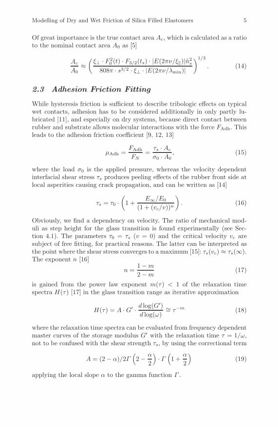
The single lines z(x) were transformed to zero level and zero slope, thenaveraged and summarized to height distributions Φ(z) (Figure 1). Althoughboth granite and asphalt have almost Gaussian distributions, asphalt is abit asymmetric and broader, which means larger height differences and thusmore vertical roughness.
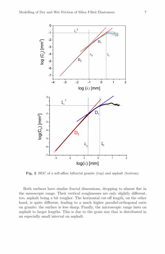
According to Equation (2) we calculated the HDC functions, which isshown in Figure 2 based on profile scans of the granite and asphalt surfaceswe used for our experiments and simulations. Both curves can be describedby two linear interpolations below their cut-offs, giving the fractal dimen-sions for their scaling ranges. The cut-off lengths are also visible. All surfaceparameters after bifractal analysis are summarized in Table 1.
Fig. 1 Height profile of granite (left) and the resulting height distribution, com-pared to asphalt (right).
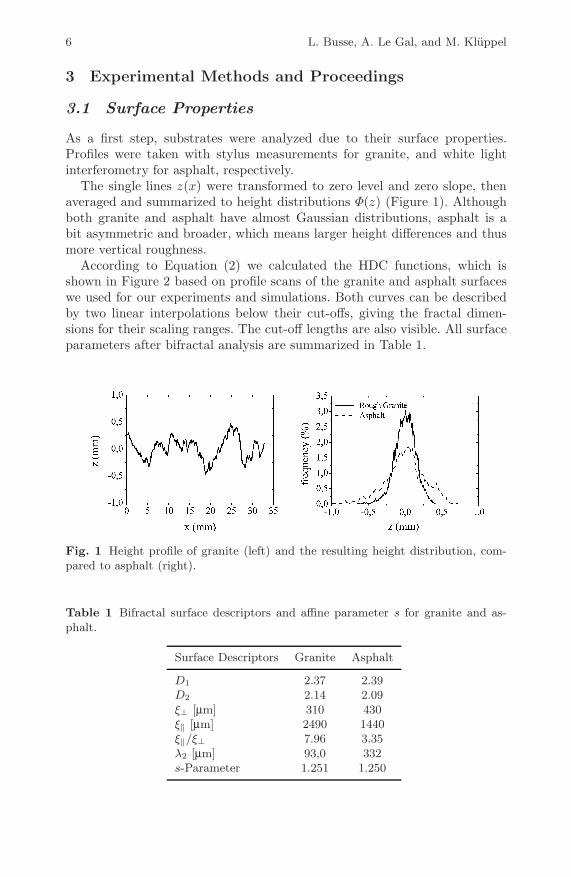
Table 1 Bifractal surface descriptors and affine parameter s for granite and as-phalt.
Surface Descriptors Granite Asphalt
D1 2.37 2.39D2 2.14 2.09ξ⊥ [μm] 310 430ξ‖ [μm] 2490 1440ξ‖/ξ⊥ 7.96 3.35λ2 [μm] 93,0 332s-Parameter 1.251 1.250
Modelling of Dry and Wet Friction of Silica Filled Elastomers 7
Fig. 2 HDC of a self-affine bifractal granite (top) and asphalt (bottom).
Both surfaces have similar fractal dimensions, dropping to almost flat inthe mesoscopic range. Their vertical roughnesses are only slightly different,too, asphalt being a bit rougher. The horizontal cut-off length, on the otherhand, is quite different, leading to a much higher parallel-orthogonal ratioon granite: the surface is less sharp. Finally, the microscopic range lasts onasphalt to larger lengths. This is due to the grain size that is distributed inan especially small interval on asphalt.
8 L. Busse, A. Le Gal, and M. Kluppel
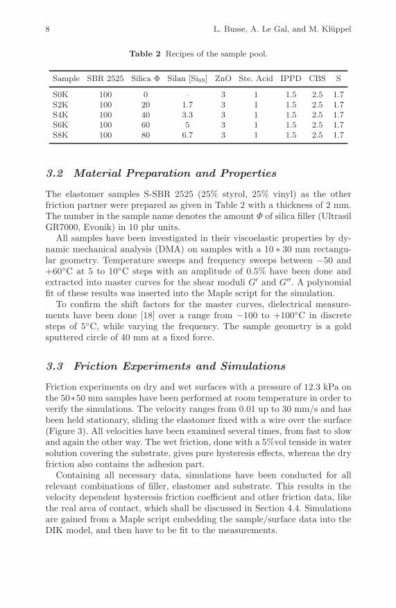
Table 2 Recipes of the sample pool.
Sample SBR 2525 Silica Φ Silan [Si69] ZnO Ste. Acid IPPD CBS S
S0K 100 0 – 3 1 1.5 2.5 1.7S2K 100 20 1.7 3 1 1.5 2.5 1.7S4K 100 40 3.3 3 1 1.5 2.5 1.7S6K 100 60 5 3 1 1.5 2.5 1.7S8K 100 80 6.7 3 1 1.5 2.5 1.7
3.2 Material Preparation and Properties
The elastomer samples S-SBR 2525 (25% styrol, 25% vinyl) as the otherfriction partner were prepared as given in Table 2 with a thickness of 2 mm.The number in the sample name denotes the amount Φ of silica filler (UltrasilGR7000, Evonik) in 10 phr units.
All samples have been investigated in their viscoelastic properties by dy-namic mechanical analysis (DMA) on samples with a 10 ∗ 30 mm rectangu-lar geometry. Temperature sweeps and frequency sweeps between −50 and+60◦C at 5 to 10◦C steps with an amplitude of 0.5% have been done andextracted into master curves for the shear moduli G′ and G′′. A polynomialfit of these results was inserted into the Maple script for the simulation.
To confirm the shift factors for the master curves, dielectrical measure-ments have been done [18] over a range from −100 to +100◦C in discretesteps of 5◦C, while varying the frequency. The sample geometry is a goldsputtered circle of 40 mm at a fixed force.
3.3 Friction Experiments and Simulations
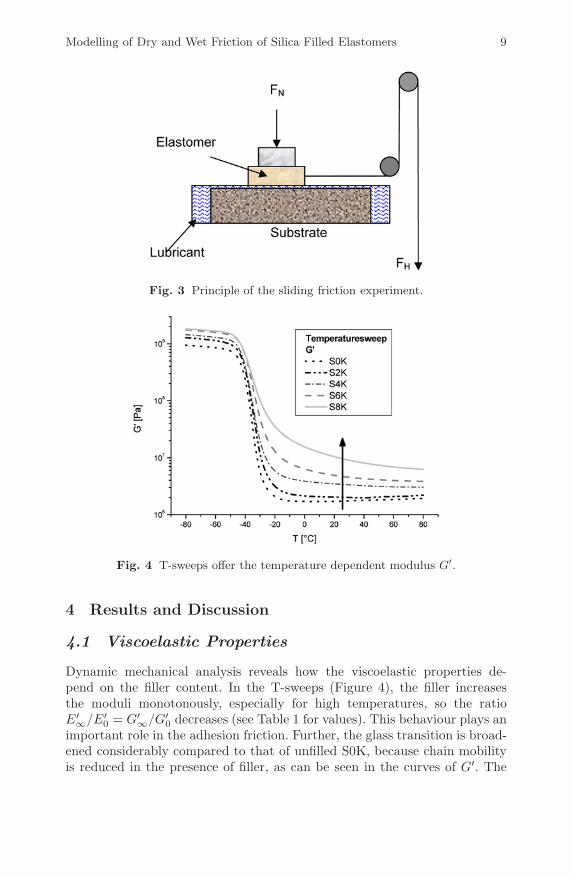
Friction experiments on dry and wet surfaces with a pressure of 12.3 kPa onthe 50∗50 mm samples have been performed at room temperature in order toverify the simulations. The velocity ranges from 0.01 up to 30 mm/s and hasbeen held stationary, sliding the elastomer fixed with a wire over the surface(Figure 3). All velocities have been examined several times, from fast to slowand again the other way. The wet friction, done with a 5%vol tenside in watersolution covering the substrate, gives pure hysteresis effects, whereas the dryfriction also contains the adhesion part.
Containing all necessary data, simulations have been conducted for allrelevant combinations of filler, elastomer and substrate. This results in thevelocity dependent hysteresis friction coefficient and other friction data, likethe real area of contact, which shall be discussed in Section 4.4. Simulationsare gained from a Maple script embedding the sample/surface data into theDIK model, and then have to be fit to the measurements.
Modelling of Dry and Wet Friction of Silica Filled Elastomers 9
Fig. 3 Principle of the sliding friction experiment.
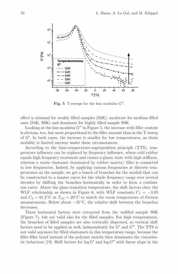
Fig. 4 T-sweeps offer the temperature dependent modulus G′.
4 Results and Discussion
4.1 Viscoelastic Properties
Dynamic mechanical analysis reveals how the viscoelastic properties de-pend on the filler content. In the T-sweeps (Figure 4), the filler increasesthe moduli monotonously, especially for high temperatures, so the ratioE′
∞/E′0 = G′
∞/G′0 decreases (see Table 1 for values). This behaviour plays an
important role in the adhesion friction. Further, the glass transition is broad-ened considerably compared to that of unfilled S0K, because chain mobilityis reduced in the presence of filler, as can be seen in the curves of G′. The
10 L. Busse, A. Le Gal, and M. Kluppel
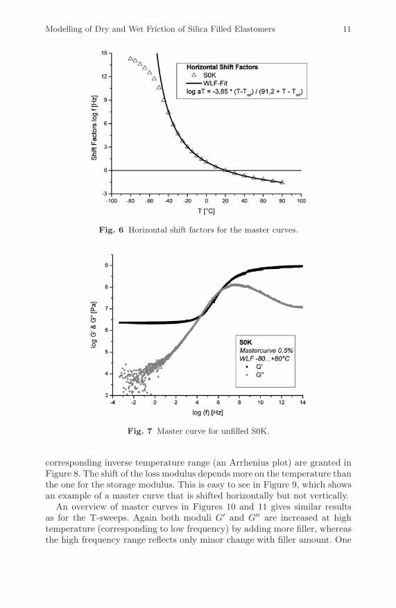
Fig. 5 T-sweeps for the loss modulus G′′.
effect is minimal for weakly filled samples (S2K), moderate for medium filledones (S4K, S6K) and dominant for highly filled sample S8K.
Looking at the loss modulus G′′ in Figure 5, the increase with filler contentis obvious, too, but more proportional to the filler amount than in the T-sweepof G′. In both cases, the increase is smaller for low temperatures, as chainmobility is limited anyway under these circumstances.
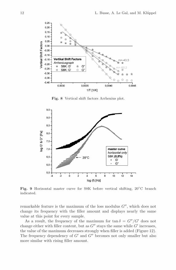
According to the time-temperature-superposition principle (TTS), tem-perature influence can be replaced by frequency influence, where cold rubberequals high frequency treatment and causes a glassy state with high stiffness,whereas a warm elastomer dominated by rubber matrix/ filler is connectedto low frequencies. Indeed, by applying various frequencies at discrete tem-peratures on the sample, we get a bunch of branches for the moduli that canbe constructed to a master curve for the whole frequency range over severaldecades by shifting the branches horizontally in order to form a continu-ous curve. Above the glass transition temperature, the shift factors obey theWLF relationship as shown in Figure 6, with WLF constants C1 = −3.85and C2 = 91.2◦C at Tref = 20◦C to match the room temperature of frictionmeasurements. Below about −45◦C, the relative shift between the branchesdecreases.
These horizontal factors were extracted from the unfilled sample S0K(Figure 7), but are valid also for the filled samples. For high temperatures,the branches of filled samples are also vertically dispersed, so vertical shiftfactors need to be applied as well, independently for G′ and G′′. The TTS isnot valid anymore for filled elastomers in this temperature range, because thefiller-filler bond instead of the polymer matrix then dominates the viscoelas-tic behaviour [19]. Shift factors for log G′ and log G′′ with linear slope in the
Modelling of Dry and Wet Friction of Silica Filled Elastomers 11
Fig. 6 Horizontal shift factors for the master curves.
Fig. 7 Master curve for unfilled S0K.
corresponding inverse temperature range (an Arrhenius plot) are granted inFigure 8. The shift of the loss modulus depends more on the temperature thanthe one for the storage modulus. This is easy to see in Figure 9, which showsan example of a master curve that is shifted horizontally but not vertically.
An overview of master curves in Figures 10 and 11 gives similar resultsas for the T-sweeps. Again both moduli G′ and G′′ are increased at hightemperature (corresponding to low frequency) by adding more filler, whereasthe high frequency range reflects only minor change with filler amount. One
12 L. Busse, A. Le Gal, and M. Kluppel
Fig. 8 Vertical shift factors Arrhenius plot.
Fig. 9 Horizontal master curve for S8K before vertical shifting, 20◦C branchindicated.
remarkable feature is the maximum of the loss modulus G′′, which does notchange its frequency with the filler amount and displays nearly the samevalue at this point for every sample.
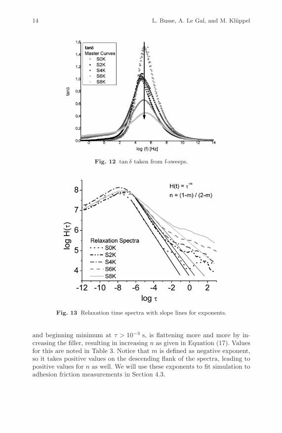
As a result, the frequency of the maximum for tan δ = G′′/G′ does notchange either with filler content, but as G′′ stays the same while G′ increases,the value of the maximum decreases strongly when filler is added (Figure 12).The frequency dependency of G′ and G′′ becomes not only smaller but alsomore similar with rising filler amount.
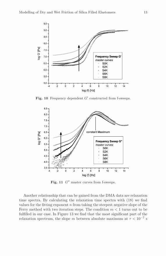
Modelling of Dry and Wet Friction of Silica Filled Elastomers 13
Fig. 10 Frequency dependent G′ constructed from f-sweeps.
Fig. 11 G′′ master curves from f-sweeps.
Another relationship that can be gained from the DMA data are relaxationtime spectra. By calculating the relaxation time spectra with (18) we findvalues for the fitting exponent n from taking the steepest negative slope of theFerry method with two iteration steps. The condition m < 1 turns out to befulfilled in our case. In Figure 13 we find that the most significant part of therelaxation spectrum, the slope m between absolute maximum at τ < 10−7 s
14 L. Busse, A. Le Gal, and M. Kluppel
Fig. 12 tan δ taken from f-sweeps.
Fig. 13 Relaxation time spectra with slope lines for exponents.
and beginning minimum at τ > 10−3 s, is flattening more and more by in-creasing the filler, resulting in increasing n as given in Equation (17). Valuesfor this are noted in Table 3. Notice that m is defined as negative exponent,so it takes positive values on the descending flank of the spectra, leading topositive values for n as well. We will use these exponents to fit simulation toadhesion friction measurements in Section 4.3.
Modelling of Dry and Wet Friction of Silica Filled Elastomers 15
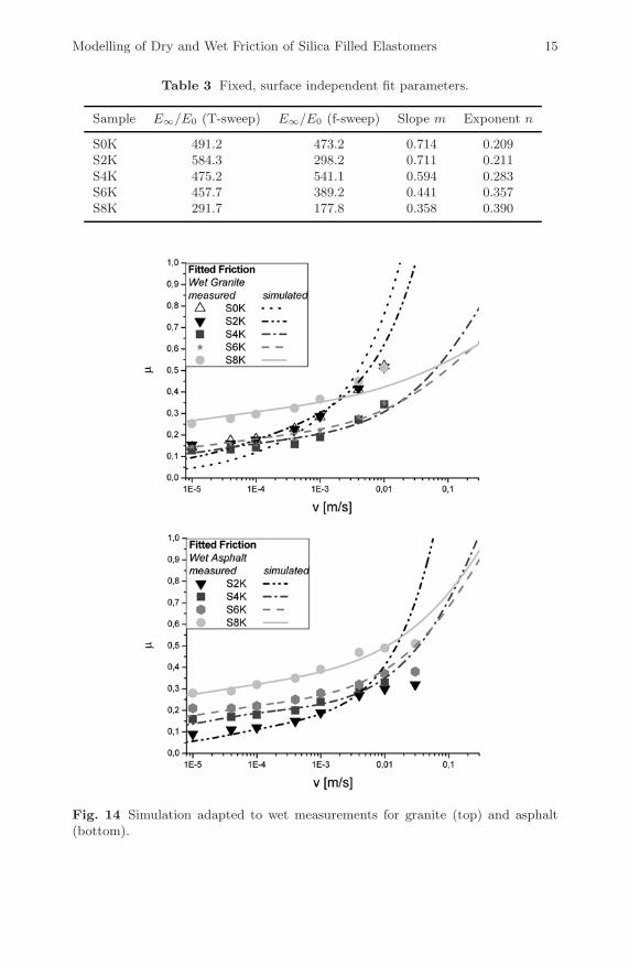
Table 3 Fixed, surface independent fit parameters.
Sample E∞/E0 (T-sweep) E∞/E0 (f-sweep) Slope m Exponent n
S0K 491.2 473.2 0.714 0.209S2K 584.3 298.2 0.711 0.211S4K 475.2 541.1 0.594 0.283S6K 457.7 389.2 0.441 0.357S8K 291.7 177.8 0.358 0.390
Fig. 14 Simulation adapted to wet measurements for granite (top) and asphalt(bottom).
16 L. Busse, A. Le Gal, and M. Kluppel
4.2 Friction Measurements
In order to investigate the pure hysteresis friction, it is necessary to extinguishadhesion friction by separating rubber from substrate so no direct molecularinteraction is possible. This can be realized by applying a low viscosity lu-bricant film. The results of these wet measurements are shown in Figure 14.On both granite and asphalt surfaces, friction clearly increases with velocity,which means lubrication is effective especially at lower speeds. In case of gran-ite the steep slope at 10 mm/s indicates a further strong increase of friction,whereas for asphalt higher velocities mean only a slight increase of friction.This is due to the lateral scaling parameter ξ‖ (see Table 3): asphalt, whichis laterally smoother than granite, exhibits the beginning of the plateau areaat lower velocities. The effect of temperature can be neglected especially onwet surfaces for most velocities in the range examined here, but might playa role for high velocities, especially without lubricant [20].
The amount of friction is similar for both substrates. In general, frictionon granite tends to be slightly higher than on asphalt. The exact behaviourstrongly depends on the filler amount: For asphalt, the friction increasesmonotonously with the degree of filler in the complete velocity range. Ongranite, this is true only when disregarding weakly filled samples (S0K, S2K).This increase of friction can be explained by the increased hysteresis of filledelastomers (see Figure 12).
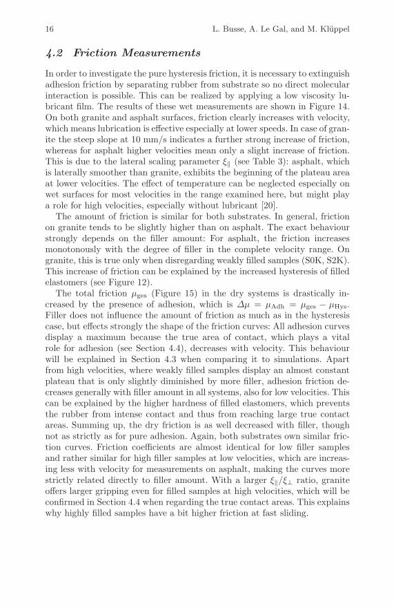
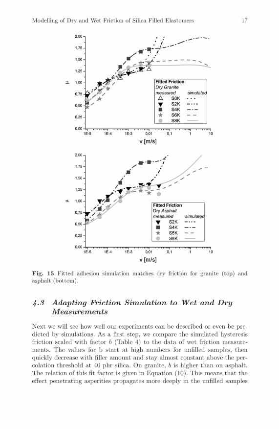
The total friction μges (Figure 15) in the dry systems is drastically in-creased by the presence of adhesion, which is Δμ = μAdh = μges − μHys.Filler does not influence the amount of friction as much as in the hysteresiscase, but effects strongly the shape of the friction curves: All adhesion curvesdisplay a maximum because the true area of contact, which plays a vitalrole for adhesion (see Section 4.4), decreases with velocity. This behaviourwill be explained in Section 4.3 when comparing it to simulations. Apartfrom high velocities, where weakly filled samples display an almost constantplateau that is only slightly diminished by more filler, adhesion friction de-creases generally with filler amount in all systems, also for low velocities. Thiscan be explained by the higher hardness of filled elastomers, which preventsthe rubber from intense contact and thus from reaching large true contactareas. Summing up, the dry friction is as well decreased with filler, thoughnot as strictly as for pure adhesion. Again, both substrates own similar fric-tion curves. Friction coefficients are almost identical for low filler samplesand rather similar for high filler samples at low velocities, which are increas-ing less with velocity for measurements on asphalt, making the curves morestrictly related directly to filler amount. With a larger ξ‖/ξ⊥ ratio, graniteoffers larger gripping even for filled samples at high velocities, which will beconfirmed in Section 4.4 when regarding the true contact areas. This explainswhy highly filled samples have a bit higher friction at fast sliding.
Modelling of Dry and Wet Friction of Silica Filled Elastomers 17
Fig. 15 Fitted adhesion simulation matches dry friction for granite (top) andasphalt (bottom).
4.3 Adapting Friction Simulation to Wet and DryMeasurements
Next we will see how well our experiments can be described or even be pre-dicted by simulations. As a first step, we compare the simulated hysteresisfriction scaled with factor b (Table 4) to the data of wet friction measure-ments. The values for b start at high numbers for unfilled samples, thenquickly decrease with filler amount and stay almost constant above the per-colation threshold at 40 phr silica. On granite, b is higher than on asphalt.The relation of this fit factor is given in Equation (10). This means that theeffect penetrating asperities propagates more deeply in the unfilled samples
18 L. Busse, A. Le Gal, and M. Kluppel
Table 4 Free fit parameters for hysteresis and adhesion simulation.
Granite Asphalt
Sample b τ0 vc b τ0 vc
– kPa mm/s – kPa mm/s
S0K 70 5.91 0.020 – – –S2K 27 6.56 0.045 10 64 0.62S4K 7 15.4 1.90 4.5 150 9.00S6K 6.8 18.8 0.90 5.5 110 0.60S8K 7.5 48.8 0.33 7 420 1.00
up to 40 phr. The simulation is shown in Figure 14 as drawn lines for all sam-ples, both on granite (top) and asphalt (bottom). Obviously, the measuredcurves can be reproduced fairly well with simulation for low and moderatevelocities, but is less accurate when sliding faster than a few mm/s: Thenthe simulations are much steeper than measurements for low fillings (S0K,S2K), more or less correct for medium fillings (S4K, S6K) and not steepenough for high fillings (S8K), on a granite surface. For asphalt, simulationsbehave the same way but are slightly steeper than on granite in comparisonto the measurements, and fit the measurements still at higher velocity. Theanswer can be found in the surface descriptors (Table 1): as ξ‖ indicates,granite is rougher than asphalt on the lateral scale, so the simulation willbe valid to higher velocities. The highly filled simulated curves are less steepand thus less dependent on velocity because their elasticity depends less ontemperature and thus less on frequency than the weakly filled samples (seeSection 4.1).
The second step is to add an adhesion term as explained in Section 2.3 tothe hysteresis fit. For the best combinations of the free and given fit parame-ters the simulation are compared to the dry measurements in Figure 15. Apartfrom the b parameters for hysteresis friction, more fit parameters were neces-sary for dry friction. Some of them could directly be taken from the results ofrubber material experiments, and do thus not depend on the contacting sur-face: the ratio E∞/E0 was measured as part of the DMA and the exponentn was extracted from relaxation time spectra as described before. Two freefit parameters, vc and τ0, were added to gain the total friction completely,individually for each surface. All surface dependent fit parameters includingb, which stays unchanged, are displayed in Table 4. The shear stress riseswith filler amount for both granite and asphalt, especially for highest fillercontent. Simulation range and accuracy of the simulation are only limited byknowledge of the regarded viscoelastic and surface properties. The criticalvelocity displays a maximum at 40 phr for both substrates.
Again, the fit is excellent for most points, even at higher velocities ongranite, but fails to mirror the fast velocities on asphalt. While temperature
Modelling of Dry and Wet Friction of Silica Filled Elastomers 19
effects by friction heating could be assumed to be neglectable on wet surfaces,they may indeed play a role on dry substrates when the sliding speed ishigh enough. The heating results in an increasing elasticity, which means thehysteresis part for dry friction is lower than for wet friction. Hysteresis frictionis still increasing with velocity, but its steepness is reduced by filled amountalready on wet surfaces. Combined with the decreasing real area of contactat high velocities, dry friction may be reduced in effect, as seen for asphaltwhen sliding fast. As a result of these two contrary effects, dry friction entersa plateau for velocities above some mm/s, as the wet part is still increasing.This behaviour has already been found by Grosch [21] as master curves ofsamples filled with 50 phr highly active carbon blacks (N220, N330) slidingon dry clean silicone and in [6] for carbon black filled S-SBR5025 on roughgranite. In our case, the same behaviour is found for the simulations of highlysilica filled systems: On granite, dry friction follows clearly this plateau shapefor the filled samples. On asphalt, the effect is present but less accented. Theeffect is confirmed by simulation and well visible on the extended velocityscale.
4.4 Contact Simulations
Apart from verifying the DIK model for friction, simulation also gives otherinteresting results, which shall be presented in this section.
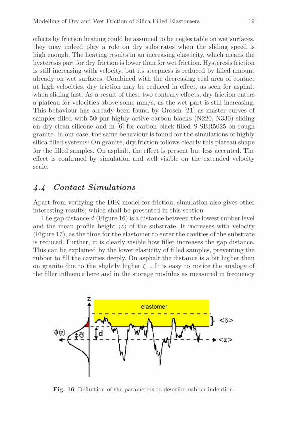
The gap distance d (Figure 16) is a distance between the lowest rubber leveland the mean profile height 〈z〉 of the substrate. It increases with velocity(Figure 17), as the time for the elastomer to enter the cavities of the substrateis reduced. Further, it is clearly visible how filler increases the gap distance.This can be explained by the lower elasticity of filled samples, preventing therubber to fill the cavities deeply. On asphalt the distance is a bit higher thanon granite due to the slightly higher ξ⊥. It is easy to notice the analogy ofthe filler influence here and in the storage modulus as measured in frequency
Fig. 16 Definition of the parameters to describe rubber indention.