Embed Size (px)
Citation preview
Lecture Notes for Ph219/CS219:Quantum Information
Chapter 5
John PreskillCalifornia Institute of Technology
Updated July 2015
Contents
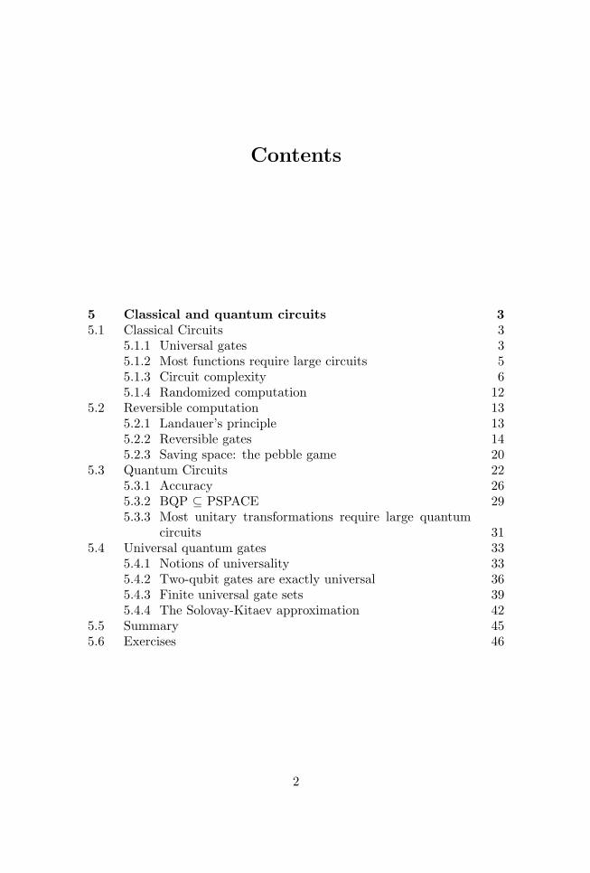
5 Classical and quantum circuits 35.1 Classical Circuits 3
5.1.1 Universal gates 35.1.2 Most functions require large circuits 55.1.3 Circuit complexity 65.1.4 Randomized computation 12
5.2 Reversible computation 135.2.1 Landauer’s principle 135.2.2 Reversible gates 145.2.3 Saving space: the pebble game 20
5.3 Quantum Circuits 225.3.1 Accuracy 265.3.2 BQP ⊆ PSPACE 295.3.3 Most unitary transformations require large quantum
circuits 315.4 Universal quantum gates 33
5.4.1 Notions of universality 335.4.2 Two-qubit gates are exactly universal 365.4.3 Finite universal gate sets 395.4.4 The Solovay-Kitaev approximation 42
5.5 Summary 455.6 Exercises 46
2
5Classical and quantum circuits
5.1 Classical Circuits
The concept of a quantum computer was introduced in Chapter 1. Herewe will specify our model of quantum computation more precisely, and wewill point out some basic properties of the model; later we will investigatethe power of the model. But before we explain what a quantum computerdoes, we should say what a classical computer does.
5.1.1 Universal gates
A (deterministic) classical computer evaluates a function: given n-bits ofinput it produces m-bits of output that are uniquely determined by theinput; that is, it finds the value of the function
f : 0, 1n → 0, 1m, (5.1)
for a particular specified n-bit argument x. A function with an m-bitoutput is equivalent to m functions, each with a one-bit output, so wemay just as well say that the basic task performed by a computer is theevaluation of
f : 0, 1n → 0, 1. (5.2)
A function talking an n-bit input to a one-bit output is called a Booleanfunction. We may think of such a function as a binary string of length 2n,where each bit of the string is the output f(x) for one of the 2n possiblevalues of the input x. Evidently, there are 22n
such strings; that’s a lot offunctions! Already for n = 5 there are 232 ≈ 4.3× 10⁹ Boolean functions— you’ve encountered only a tiny fraction of these in your lifetime.
It is sometimes useful to regard a Boolean function as a subset Σ of then-bit strings containing those values of the input x such that f(x) = 1; we
3
4 5 Classical and quantum circuits
say these strings are “accepted” by f . The complementary set Σ containsvalues of x such that f(x) = 0, which we say are “rejected” by f .
The evaluation of a Boolean function f can be reduced to a sequence ofsimple logical operations. To see how, denote the n-bit strings acceptedby f as Σ = x(1), x(2), x(3), . . . and note that for each x(a) we can definea function f (a) : 0, 1n → 0, 1 such that
f (a)(x) =
1 x = x(a)
0 otherwise(5.3)
Then f can be expressed as
f(x) = f (1)(x) ∨ f (2)(x) ∨ f (3)(x) ∨ . . . , (5.4)
the logical OR (∨) of all the f (a)’s. In binary arithmetic the ∨ operationof two bits may be represented
x ∨ y = x+ y − x · y; (5.5)
it has the value 0 if x and y are both zero, and the value 1 otherwise.Now consider the evaluation of f (a). We express the n-bit string x as
x = xn−1xn−2 . . . x2x1x0. (5.6)
In the case where x(a) = 11 . . . 111, we may write
f (a)(x) = xn−1 ∧ xn−2 ∧ . . . ∧ x2 ∧ x1 ∧ x0; (5.7)
it is the logical AND (∧) of all n bits. In binary arithmetic, the AND isthe product
x ∧ y = x · y. (5.8)
For any other x(a), f (a) is again obtained as the AND of n bits, but wherethe NOT (¬) operation is first applied to each xi such that x(a)
i = 0; forexample
f (a)(x) = . . . (¬x3) ∧ x2 ∧ x1 ∧ (¬x0) (5.9)
ifx(a) = . . . 0110. (5.10)
The NOT operation is represented in binary arithmetic as
¬x = 1− x. (5.11)
We have now constructed the function f(x) from three elementary log-ical connectives: NOT, AND, OR. The expression we obtained is calledthe “disjunctive normal form” (DNF) of f(x). We have also implicitlyused another operation INPUT(xi), which inputs the ith bit of x.
5.1 Classical Circuits 5
These considerations motivate the circuit model of computation. Acomputer has a few basic components that can perform elementary oper-ations on bits or pairs of bits, such as NOT, AND, OR. It can also input avariable bit or prepare a constant bit. A computation is a finite sequenceof such operations, a circuit, applied to a specified string of input bits.Each operation is called a gate. The result of the computation is the finalvalue of all remaining bits, after all the elementary operations have beenexecuted. For a Boolean function (with a one-bit output), if there aremultiple bits still remaining at the end of the computation, one is desig-nated as the output bit. A circuit can be regarded as a directed acyclicgraph, where each vertex in the graph is a gate, and the directed edgesindicate the flow of bits through the circuit, with the direction specifyingthe order in which gates are applied. By acyclic we mean that no directedclosed loops are permitted.
We say that the gate set NOT, AND, OR, INPUT is “universal,”meaning that any function can be evaluated by building a circuit fromthese components. It is a remarkable fact about the world that an arbi-trary computation can be performed using such simple building blocks.
5.1.2 Most functions require large circuits
Our DNF construction shows that any Boolean function with an n-bitinput can be evaluated using no more than 2n OR gates, n2n AND gates,n2n NOT gates, and n2n INPUT gates, a total of (3n + 1)2n gates. Ofcourse, some functions can be computed using much smaller circuits, butfor most Boolean functions the smallest circuit that evaluates the functionreally does have an exponentially large (in n) number of gates. The pointis that if the circuit size (i.e., number of gates) is subexponential in n,then there are many, many more functions than circuits.
How many circuits are there with G gates acting on an n-bit input?Consider the gate set from which we constructed the DNF, where we willalso allow inputting of a constant bit (either 0 or 1) in case we want touse some scratch space when we compute. Then there are n+ 5 differentgates: NOT, AND, OR, INPUT(0), INPUT(1), and INPUT(xi) for i =0, 1, 2, . . . n − 1. Each two-qubit gate acts on a pair of bits which areoutputs from preceding gates; this pair can be chosen in fewer than G2
ways. Therefore the total number of size-G circuits can be bounded as
Ncircuit(G) ≤((n+ 5)G2
)G. (5.12)
6 5 Classical and quantum circuits
If G = c2n
2n , where c is a constant independent of n, then
log2Ncircuit(G) ≤ G (log2(n+ 5) + 2 log2G)
= c2n
(1 +
12n
log2
(c2(n+ 5)
4n2
))≤ c2n, (5.13)
where the second inequality holds for n sufficiently large. Comparing withthe number of Boolean functions, Nfunction(n) = 22n
, we find
log2
(Ncircuit(G)Nfunction(n)
)≤ (c− 1)2n (5.14)
for n sufficiently large. Therefore, for any c < 1, the number of circuitsis smaller than the number of functions by a huge factor. We did thisanalysis for one particular universal gate set, but the counting wouldnot have been substantially different if we had used a different gate setinstead.
We conclude that for any positive ε, then, most Boolean functions re-quire circuits with at least (1 − ε)2n
2n gates. The circuit size is so largebecause most functions have no structure that can be exploited to con-struct a more compact circuit. We can’t do much better than consultinga “look-up table” that stores a list of all accepted strings, which is essen-tially what the DNF does.
5.1.3 Circuit complexity
So far, we have only considered a computation that acts on an input witha fixed (n-bit) size, but we may also consider families of circuits that acton inputs of variable size. Circuit families provide a useful scheme foranalyzing and classifying the complexity of computations, a scheme thatwill have a natural generalization when we turn to quantum computation.
Boolean functions arise naturally in the study of complexity. A Booleanfunction f may be said to encode a solution to a “decision problem” — thefunction examines the input and issues a YES or NO answer. Often, whatmight not be stated colloquially as a question with a YES/NO answer canbe “repackaged” as a decision problem. For example, the function thatdefines the FACTORING problem is:
f(x, y) =
1 if integer x has a divisor z such that 1 < z < y,0 otherwise;
(5.15)knowing f(x, y) for all y < x is equivalent to knowing the least nontrivialfactor of x (if there is one).
5.1 Classical Circuits 7
Another example of a decision problem is the HAMILTONIAN PATHproblem: let the input be an `-vertex graph, represented by an ` × `adjacency matrix ( a 1 in the ij entry means there is an edge linkingvertices i and j); the function is
f(x) =
1 if graph x has a Hamiltonian path,0 otherwise. (5.16)
A path on the graph is Hamiltonian if it visits each vertex exactly once.For the FACTORING problem the size of the input is the number of
bits needed to specify x and y, while for the HAMILTONIAN PATHproblem the size of the input is the number of bits needed to specify thegraph. Thus each problem really defines a family of Boolean functionswith variable input size. We denote such a function family as
f : 0, 1∗ → 0, 1, (5.17)
where the ∗ indicates that the input size is variable. When x is an n-bit string, by writing f(x) we mean the Boolean function in the familywhich acts on an n-bit input is evaluated for input x. The set L of stringsaccepted by a function family
L = x ∈ 0, 1∗ : f(x) = 1 (5.18)
is called a language.We can quantify the hardness of a problem by stating how the compu-
tational resources needed to solve the problem scale with the input sizen. In the circuit model of computation, it is natural to use the circuit size(number of gates) to characterize the required resources. Alternatively,we might be interested in how much time it takes to do the computation ifmany gates can be executed in parallel; the depth of a circuit is the num-ber of time steps required, assuming that gates acting on distinct bits canoperate simultaneously (that is, the depth is the maximum length of adirected path from the input to the output of the circuit). The width of acircuit, the maximum number of gates (including identity gates acting on“resting” bits) that act in any one time step, quantifies the storage spaceused to execute the computation.
We would like to divide the decision problems into two classes: easyand hard. But where should we draw the line? For this purpose, weconsider decision problems with variable input size, where the number ofbits of input is n, and examine how the size of the circuit that solves theproblem scales with n.
If we use the scaling behavior of a circuit family to characterize thedifficulty of a problem, there is a subtlety. It would be cheating to hide thedifficulty of the problem in the design of the circuit. Therefore, we should
8 5 Classical and quantum circuits
restrict attention to circuit families that have acceptable “uniformity”properties — it must be “easy” to build the circuit with n + 1 bits ofinput once we have constructed the circuit with an n-bit input.
Associated with a family of functions fn (where fn has n-bit input)are circuits Cn that compute the functions. We say that a circuit familyCn is “polynomial size” if the size |Cn| of Cn grows with n no fasterthan a power of n,
size (Cn) ≤ poly(n), (5.19)
where poly denotes a polynomial. Then we define:
P = decision problems solved by polynomial-sizeuniform circuit families
(P for “polynomial time”). Decision problems in P are “easy.” The restare “hard.” Notice that Cn computes fn(x) for every possible n-bit input,and therefore, if a decision problem is in P we can find the answer even forthe “worst-case” input using a circuit of size no greater than poly(n). Asalready noted, we implicitly assume that the circuit family is “uniform”so that the design of the circuit can itself be solved by a polynomial-time algorithm. Under this assumption, solvability in polynomial timeby a circuit family is equivalent to solvability in polynomial time by auniversal Turing machine.
Of course, to determine the size of a circuit that computes fn, we mustknow what the elementary components of the circuit are. Fortunately,though, whether a problem lies in P does not depend on what gate setwe choose, as long as the gates are universal, the gate set is finite, andeach gate acts on a constant number of bits. One universal gate set cansimulate another efficiently.
The way of distinguishing easy and hard problems may seem rather ar-bitrary. If |Cn| ∼ n1000 we might consider the problem to be intractable inpractice, even though the scaling is “polynomial,” and if |Cn| ∼ nlog log log n
we might consider the problem to be easy in practice, even though thescaling is “superpolynomial.” Furthermore, even if |Cn| scales like a mod-est power of n, the constants in the polynomial could be very large. Suchpathological cases seem to be uncommon, however. Usually polynomialscaling is a reliable indicator that solving the problem is feasible.
Of particular interest are decision problems that can be answered byexhibiting an example that is easy to verify. For example, given x andy < x, it is hard (in the worst case) to determine if x has a factor less thany. But if someone kindly provides a z < y that divides x, it is easy for usto check that z is indeed a factor of x. Similarly, it is hard to determine ifa graph has a Hamiltonian path, but if someone kindly provides a path,it is easy to verify that the path really is Hamiltonian.
5.1 Classical Circuits 9
This concept that a problem may be hard to solve, but that a solutioncan be easily verified once found, can be formalized. The complexity classof decision problems for which the answer can be checked efficiently, calledNP, is defined as
Definition. NP. A language L is in NP iff there is a polynomial-sizeverifier V (x, y) such that
If x ∈ L, then there exists y such that V (x, y) = 1 (completeness),
If x 6∈ L, then, for all y, V (x, y) = 0 (soundness).
The verifier V is the uniform circuit family that checks the answer. Com-pleteness means that for each input in the language (for which the answeris YES), there is an appropriate “witness” such that the verifier acceptsthe input if that witness is provided. Soundness means that for each inputnot in the language (for which the answer is NO) the verifier rejects theinput no matter what witness is provided. It is implicit that the witnessis of polynomial length, |y| = poly(|x|); since the verifier has a polynomialnumber of gates, including input gates, it cannot make use of more thana polynomial number of bits of the witness. NP stands for “nondeter-ministic polynomial time;” this name is used for historical reasons, butit is a bit confusing since the verifier is actually a deterministic circuit(evaluates a function).
If is obvious that P ⊆ NP; if the problem is in P then the polynomial-time verifier can decide whether to accept x on its own, without anyhelp from the witness. But some problems in NP seem to be hard, andare believed not to be in P. Much of complexity theory is built on afundamental conjecture:
Conjecture : P 6= NP. (5.20)
Proving or refuting this conjecture is the most important open problemin computer science, and one of the most important problems in mathe-matics.
Why should we believe P 6= NP? If P = NP that would mean we couldeasily find the solution to any problem whose solution is easy to check. Ineffect, then, we could automate creativity; in particular, computers wouldbe able to discover all the mathematical theorems which have short proofs.The conjecture P 6= NP asserts that our machines will never achievesuch awesome power — that the mere existence of a succinct proof of astatement does not ensure that we can find the proof by any systematicprocedure in any reasonable amount of time.
An important example of a problem in NP is CIRCUIT-SAT. In thiscase the input is a Boolean circuit C, and the problem is to determine
10 5 Classical and quantum circuits
whether any input x is accepted by C. The function to be evaluated is
f(C) =
1 if there exists x with C(x) = 1,0 otherwise. (5.21)
This problem is in NP because if the circuit C has polynomial size, thenif we are provided with an input x accepted by C it is easy to check thatC(x) = 1.
The problem CIRCUIT-SAT is particularly interesting because it has aremarkable property — if we have a machine that solves CIRCUIT-SATwe can use it to solve any other problem in NP. We say that every problemin NP is (efficiently) reducible to CIRCUIT-SAT. More generally, we saythat problem B reduces to problem A if a machine that solves A can beused to solve B as well.
That is, if A and B are Boolean function families, then “B reduces toA” means there is a function family R, computed by poly-size circuits,such that B(x) = A(R(x)). Thus B accepts x iff A accepts R(x). Inparticular, then, if we have a poly-size circuit family that solves A, wecan hook A up with R to obtain a poly-size circuit family that solves B.
A problem B in NP reduces to CIRCUIT-SAT because problem B hasa poly-size verifier V (x, y), such that B accepts x iff there exists somewitness y such that V accepts (x, y). For each fixed x, asking whethersuch a witness y exists is an instance of CIRCUIT-SAT. So a poly-sizecircuit family that solves CIRCUIT-SAT can also be used to solve problemB.
We say a problem A in NP is NP-complete if every problem in NP isreducible to A. Hence, CIRCUIT-SAT is NP-complete. The NP-completeproblems are the “hardest” problems in NP, in the sense that if we cansolve any NP-complete problem then we can solve every NP problem.Furthermore, to show that problem A is NP-complete, it is enough toshow that B reduces to A where B is NP-complete. If C is any problem inNP and B is NP-complete then there is a poly-size reduction R such thatC(x) = B(R(x)), and if B is reducible to A then there is another poly-sizereduction R′ such that B(y) = A(R′(y)). Hence C(x) = A(R′(R(x))), andsince the composition R′ R of two poly-size reductions is also poly-size,we see that an arbitrary problem C in NP reduces to A, and therefore Ais NP-complete. NP-completeness is a useful concept because hundredsof “natural” computational problems turn out to be NP-complete. Forexample, one can exhibit a polynomial reduction of CIRCUIT-SAT toHAMILTONIAN PATH, and it follows that HAMILTONIAN PATH isalso NP-complete.
Another noteworthy complexity class is called co-NP. While NP prob-lems can be decided by exhibiting an example if the answer is YES, co-NP
5.1 Classical Circuits 11
problems can be answered by exhibiting a counter-example if the answeris NO. More formally:
Definition. co-NP. A language L is in co-NP iff there is a polynomial-size verifier V (x, y) such that
If x 6∈ L, then there exists y such that V (x, y) = 1,
If x ∈ L, then, for all y, V (x, y) = 0.
For NP the witness y testifies that x is in the language while for co-NPthe witness testifies that x is not in the language. Thus if language L isin NP, then its complement L is in co-NP and vice-versa. We see thatwhether we consider a problem to be in NP or in co-NP depends on howwe choose to frame the question — while “Is there a Hamiltonian path?”is in NP, the complementary question “Is there no Hamiltonian path?” isin co-NP.
Though the distinction between NP and co-NP may seem arbitrary, itis nevertheless interesting to ask whether a problem is in both NP andco-NP. If so, then we can easily verify the answer (once a suitable witnessis in hand) regardless of whether the answer is YES or NO. It is believed(though not proved) that NP 6= co-NP. For example, we can show thata graph has a Hamiltonian path by exhibiting an example, but we don’tknow how to show that it has no Hamiltonian path that way!
If we assume that P 6= NP, it is known that there exist problems inNP of intermediate difficulty (the class NPI), which are neither in P norNP-complete. Furthermore, assuming that that NP 6= co-NP, it is knownthat no co-NP problems are NP-complete. Therefore, problems in theintersection of NP and co-NP, if not in P, are good candidates for inclusionin NPI.
In fact, a problem in NP ∩ co-NP believed not to be in P is the FAC-TORING problem. As already noted, FACTORING is in NP because,if we are offered a factor of x, we can easily check its validity. But it isalso in co-NP, because it is known that if we are given a prime numberwe can efficiently verify its primality. Thus, if someone tells us the primefactors of x, we can efficiently check that the prime factorization is right,and can exclude that any integer less than y is a divisor of x. Therefore,it seems likely that FACTORING is in NPI.
We are led to a crude (conjectured) picture of the structure of NP ∪ co-NP. NP and co-NP do not coincide, but they have a nontrivial intersection.P lies in NP ∩ co-NP but the intersection also contains problems not inP (like FACTORING). No NP-complete or co-NP-complete problems liein NP ∩ co-NP.
12 5 Classical and quantum circuits
5.1.4 Randomized computation
It is sometimes useful to consider probabilistic circuits that have accessto a random number generator. For example, a gate in a probabilisticcircuit might act in either one of two ways, and flip a fair coin to decidewhich action to execute. Such a circuit, for a single fixed input, cansample many possible computational paths. An algorithm performed bya probabilistic circuit is said to be “randomized.”
If we run a randomized computation many times on the same input,we won’t get the same answer every time; rather there is a probabilitydistribution of outputs. But the computation is useful if the probabilityof getting the right answer is high enough. For a decision problem, wewould like a randomized computation to accept an input x which is inthe language L with probability at least 1
2 + δ, and to accept an inputx which is not in the language with probability no greater than 1
2 − δ,where δ > 0 is a constant independent of the input size. In that casewe can amplify the probability of success by performing the computationmany times and taking a majority vote on the outcomes. For x ∈ L, if werun the computation N times, the probability of rejecting in more thanhalf the runs is no more than e−2Nδ2
(the Chernoff bound). Likewise, forx 6∈ L, the probability of accepting in the majority of N runs is no morethan e−2Nδ2
.Why? There are all together 2N possible sequences of outcomes in the
N trials, and the probability of any particular sequence with NW wronganswers is (
12− δ
)NW(
12
+ δ
)N−NW
. (5.22)
The majority is wrong only if NW ≥ N/2, so the probability of anysequence with an incorrect majority is no larger than(
12− δ
)N/2(12
+ δ
)N/2
=1
2N
(1− 4δ2
)N/2. (5.23)
Using 1− x ≤ e−x and multiplying by the total number of sequences 2N ,we obtain the Chernoff bound:
Prob(wrong majority) ≤(1− 4δ2
)N/2 ≤ e−2Nδ2. (5.24)
If we are willing to accept a probability of error no larger than ε, then,it suffices to run the computation a number of times
N ≥ 12δ2
ln (1/ε) . (5.25)

5.2 Reversible computation 13
Because we can make the error probability very small by repeating arandomized computation a modest number of times, the value of the con-stant δ does not really matter for the purpose of classifying complexity,as long as it is positive and independent of the input size. The standardconvention is to specify δ = 1/6, so that x ∈ L is accepted with proba-bility at least 2/3 and x 6∈ L is accepted with probability no more than1/3. This criterion defines the class BPP (“bounded-error probabilisticpolynomial time”) containing decision problems solved by polynomial-sizerandomized uniform circuit families.
It is clear that BPP contains P, since a deterministic computation is aspecial case of a randomized computation, in which we never consult thesource of randomness. It is widely believed that BPP=P, that randomnessdoes not enhance our computational power, but this has not been proven.It is not even known whether BPP is contained in NP.
We may define a randomized class analogous to NP, called MA(“Merlin-Arthur”), containing languages that can be checked when a ran-domized verifier is provided with a suitable witness:
Definition. MA. A language L is in MA iff there is a polynomial-sizerandomized verifier V (x, y) such that
If x ∈ L, then there exists y such that Prob(V (x, y) = 1) ≥ 2/3,If x 6∈ L, then, for all y, Prob(V (x, y) = 1) ≤ 1/3.
The colorful name evokes a scenario in which the all-powerful Merlin useshis magical powers to conjure the witness, allowing the mortal Arthur,limited to polynomial time computation, to check the answer. ObviouslyBPP is contained in MA, but we expect BPP 6= MA just as we expect P6= NP.
5.2 Reversible computation
In devising a model of a quantum computer, we will generalize the cir-cuit model of classical computation. But our quantum logic gates willbe unitary transformations, and hence will be invertible, while classicallogic gates like the AND gate are not invertible. Before we discuss quan-tum circuits, it is useful to consider some features of reversible classicalcomputation.
5.2.1 Landauer’s principle
Aside from providing a bridge to quantum computation, classical re-versible computing is interesting in its own right, because of Landauer’sprinciple. Landauer observed that erasure of information is necessarily a
14 5 Classical and quantum circuits
dissipative process. His insight is that erasure always involves the com-pression of phase space, and so is thermodynamically, as well as logically,irreversible.
For example, I can store one bit of information by placing a singlemolecule in a box, either on the left side or the right side of a partition thatdivides the box. Erasure means that we move the molecule to the rightside (say) irrespective of whether it started out on the left or right. I cansuddenly remove the partition, and then slowly compress the one-molecule“gas” with a piston until the molecule is definitely on the right side. Thisprocedure changes the entropy of the gas by ∆S = −k ln 2 (where k isBoltzmann’s constant) and there is an associated flow of heat from thebox to its environment. If the process is quasi-static and isothermal attemperature T , then work W = −kT∆S = kT ln 2 is performed on thebox, work that I have to provide. If I erase information, someone has topay the power bill.
Landauer also observed that, because irreversible logic elements eraseinformation, they too are necessarily dissipative, and therefore require anunavoidable expenditure of energy. For example, an AND gate maps twoinput bits to one output bit, with 00, 01, and 10 all mapped to 0, while11 is mapped to one. If the input is destroyed and we can read only theoutput, then if the output is 0 we don’t know for sure what the input was— there are three possibilities. If the input bits are chosen uniformly atrandom, than on average the AND gate destroys 3
4 log2 3 ≈ 1.189 bits ofinformation. Indeed, if the input bits are uniformly random any 2-to-1gate must “erase” at least one bit on average. According to Landauer’sprinciple, then, we need to do an amount of work at least W = kT ln 2 tooperate a 2-to-1 logic gate at temperature T .
But if a computer operates reversibly, then in principle there need beno dissipation and no power requirement. We can compute for free! Atpresent this idea is not of great practical importance, because the powerconsumed in today’s integrated circuits exceeds kT per logic gate by atleast three orders of magnitude. As the switches on chips continue toget smaller, though, reversible computing might eventually be invoked toreduce dissipation in classical computing hardware.
5.2.2 Reversible gates
A reversible computer evaluates an invertible function taking n bits to nbits
f : 0, 1n → 0, 1n . (5.26)
An invertible function has a unique input for each output, and we canrun the computation backwards to recover the input from the output. We
5.2 Reversible computation 15
may regard an invertible function as a permutation of the 2n strings ofn bits — there are (2n)! such functions. If we did not insist on invert-ibility, there would be
(22n)n = (2n)2
n
functions taking n bits to n bits(the number of ways to choose n Boolean functions); using the Stirlingapproximation, (2n)! ≈ (2n/e)2
n, we see that the fraction of all functions
which are invertible is quite small, about e−2n.
Any irreversible computation can be “packaged” as an evaluation of aninvertible function. For example, for any f : 0, 1n → 0, 1, we canconstruct f : 0, 1n+1 → 0, 1n+1 such that
f(x, y) = (x, y ⊕ f(x)). (5.27)
Here y is a bit and ⊕ denotes the XOR gate (addition mod 2) — then-bit input x is preserved and the last bit flips iff f(x) = 1. Applying fa second time undoes this bit flip; hence f is invertible, and equal to itsown inverse. If we set y = 0 initially and apply f , we can read out thevalue of f(x) in the last output bit.
Just as for Boolean functions, we can ask whether a complicated re-versible computation can be executed by a circuit built from simple com-ponents — are there universal reversible gates? It is easy to see thatone-bit and two-bit reversible gates do not suffice; we will need three-bitgates for universal reversible computation.
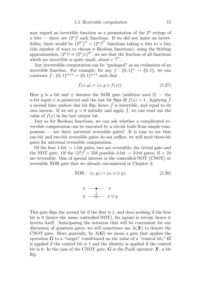
Of the four 1-bit → 1-bit gates, two are reversible; the trivial gate andthe NOT gate. Of the (24)2 = 256 possible 2-bit → 2-bit gates, 4! = 24are reversible. One of special interest is the controlled-NOT (CNOT) orreversible XOR gate that we already encountered in Chapter 4:
XOR : (x, y) 7→ (x, x⊕ y), (5.28)
x
y
x
x⊕ y
sgThis gate flips the second bit if the first is 1, and does nothing if the firstbit is 0 (hence the name controlled-NOT). Its square is trivial; hence itinverts itself. Anticipating the notation that will be convenient for ourdiscussion of quantum gates, we will sometimes use Λ(X) to denote theCNOT gate. More generally, by Λ(G) we mean a gate that applies theoperation G to a “target” conditioned on the value of a “control bit;” Gis applied if the control bit is 1 and the identity is applied if the controlbit is 0. In the case of the CNOT gate, G is the Pauli operator X, a bitflip.
16 5 Classical and quantum circuits
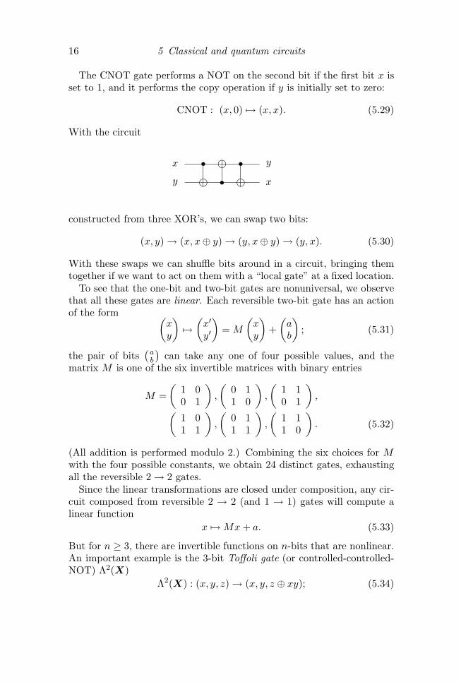
The CNOT gate performs a NOT on the second bit if the first bit x isset to 1, and it performs the copy operation if y is initially set to zero:
CNOT : (x, 0) 7→ (x, x). (5.29)
With the circuit
x
y
y
x
sg gs sgconstructed from three XOR’s, we can swap two bits:
(x, y) → (x, x⊕ y) → (y, x⊕ y) → (y, x). (5.30)
With these swaps we can shuffle bits around in a circuit, bringing themtogether if we want to act on them with a “local gate” at a fixed location.
To see that the one-bit and two-bit gates are nonuniversal, we observethat all these gates are linear. Each reversible two-bit gate has an actionof the form (
xy
)7→(x′
y′
)= M
(xy
)+(ab
); (5.31)
the pair of bits(
ab
)can take any one of four possible values, and the
matrix M is one of the six invertible matrices with binary entries
M =(
1 00 1
),
(0 11 0
),
(1 10 1
),(
1 01 1
),
(0 11 1
),
(1 11 0
). (5.32)
(All addition is performed modulo 2.) Combining the six choices for Mwith the four possible constants, we obtain 24 distinct gates, exhaustingall the reversible 2 → 2 gates.
Since the linear transformations are closed under composition, any cir-cuit composed from reversible 2 → 2 (and 1 → 1) gates will compute alinear function
x 7→Mx+ a. (5.33)
But for n ≥ 3, there are invertible functions on n-bits that are nonlinear.An important example is the 3-bit Toffoli gate (or controlled-controlled-NOT) Λ2(X)
Λ2(X) : (x, y, z) → (x, y, z ⊕ xy); (5.34)
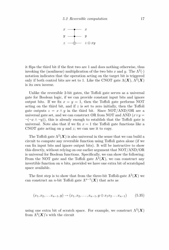
5.2 Reversible computation 17
x
y
z
x
y
z ⊕ xy
ssg
it flips the third bit if the first two are 1 and does nothing otherwise, thusinvoking the (nonlinear) multiplication of the two bits x and y. The Λ2(·)notation indicates that the operation acting on the target bit is triggeredonly if both control bits are set to 1. Like the CNOT gate Λ(X), Λ2(X)is its own inverse.
Unlike the reversible 2-bit gates, the Toffoli gate serves as a universalgate for Boolean logic, if we can provide constant input bits and ignoreoutput bits. If we fix x = y = 1, then the Toffoli gate performs NOTacting on the third bit, and if z is set to zero initially, then the Toffoligate outputs z = x ∧ y in the third bit. Since NOT/AND/OR are auniversal gate set, and we can construct OR from NOT and AND (x∨y =¬(¬x ∧ ¬y)), this is already enough to establish that the Toffoli gate isuniversal. Note also that if we fix x = 1 the Toffoli gate functions like aCNOT gate acting on y and z; we can use it to copy.
The Toffoli gate Λ2(X) is also universal in the sense that we can build acircuit to compute any reversible function using Toffoli gates alone (if wecan fix input bits and ignore output bits). It will be instructive to showthis directly, without relying on our earlier argument that NOT/AND/ORis universal for Boolean functions. Specifically, we can show the following:From the NOT gate and the Toffoli gate Λ2(X), we can construct anyinvertible function on n bits, provided we have one extra bit of scratchpadspace available.
The first step is to show that from the three-bit Toffoli-gate Λ2(X) wecan construct an n-bit Toffoli gate Λn−1(X) that acts as
(x1, x2, . . . xn−1, y) → (x1, x2, . . . , xn−1, y ⊕ x1x2 . . . xn−1) (5.35)
using one extra bit of scratch space. For example, we construct Λ3(X)from Λ2(X)’s with the circuit
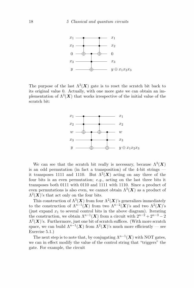
18 5 Classical and quantum circuits
x1
x2
0
x3
y
x1
x2
0
x3
y ⊕ x1x2x3
ssg ssg
ssg
The purpose of the last Λ3(X) gate is to reset the scratch bit back toits original value 0. Actually, with one more gate we can obtain an im-plementation of Λ3(X) that works irrespective of the initial value of thescratch bit:
x1
x2
w
x3
y
x1
x2
w
x3
y ⊕ x1x2x3
ssg ssg
ssg ssgWe can see that the scratch bit really is necessary, because Λ3(X)
is an odd permutation (in fact a transposition) of the 4-bit strings —it transposes 1111 and 1110. But Λ2(X) acting on any three of thefour bits is an even permutation; e.g., acting on the last three bits ittransposes both 0111 with 0110 and 1111 with 1110. Since a product ofeven permutations is also even, we cannot obtain Λ3(X) as a product ofΛ2(X)’s that act only on the four bits.
This construction of Λ3(X) from four Λ2(X)’s generalizes immediatelyto the construction of Λn−1(X) from two Λn−2(X)’s and two Λ2(X)’s(just expand x1 to several control bits in the above diagram). Iteratingthe construction, we obtain Λn−1(X) from a circuit with 2n−2 + 2n−3− 2Λ2(X)’s. Furthermore, just one bit of scratch suffices. (With more scratchspace, we can build Λn−1(X) from Λ2(X)’s much more efficiently — seeExercise 5.1.)
The next step is to note that, by conjugating Λn−1(X) with NOT gates,we can in effect modify the value of the control string that “triggers” thegate. For example, the circuit

5.2 Reversible computation 19
x1
x2
x3
y
gg
sssg
gg
flips the value of y if x1x2x3 = 010, and it acts trivially otherwise. Thusthis circuit transposes the two strings 0100 and 0101. In like fashion, withΛn−1(X) and NOT gates, we can devise a circuit that transposes any twon-bit strings that differ in only one bit. (The location of the bit wherethey differ is chosen to be the target of the Λn−1(X) gate.)
But in fact a transposition that exchanges any two n-bit strings canbe expressed as a product of transpositions that interchange strings thatdiffer in only one bit. If a0 and as are two strings that are Hammingdistance s apart (differ in s places), then there is a sequence of strings
a0, a1, a2, a3, . . . , as, (5.36)
such that each string in the sequence is Hamming distance one from itsneighbors. Therefore, each of the transpositions
(a0a1), (a1a2), (a2a3), . . . , (as−1as), (5.37)
can be implemented as a Λn−1(X) gate conjugated by NOT gates. Bycomposing transpositions we find
(a0as) = (as−1as)(as−2as−1) . . . (a2a3)(a1a2)(a0a1)(a1a2)(a2a3). . . (as−2as−1)(as−1as); (5.38)
we can construct the Hamming-distance-s transposition from 2s − 1Hamming-distance-one transpositions. It follows that we can construct(a0as) from Λn−1(X)’s and NOT gates.
Finally, since every permutation is a product of transpositions, we haveshown that every invertible function on n-bits (every permutation of then-bit strings) is a product of Λn−1(X)’s and NOT’s, using just one bit ofscratch space.
Of course, a NOT can be performed with a Λ2(X) gate if we fix twoinput bits at 1. Thus the Toffoli gate Λ2(X) is universal for reversiblecomputation, if we can fix input bits and discard output bits.
20 5 Classical and quantum circuits
5.2.3 Saving space: the pebble game
We have seen that with Toffoli and NOT gates we can compute any in-vertible function using very little scratch space, and also that by fixingconstant input bits and ignoring output bits, we can simulate any (irre-versible) Boolean circuit using only reversible Toffoli gates. In the lattercase, though, we generate two bits of junk every time we simulate anAND gate. Our memory gradually fills with junk, until we reach thestage where we cannot continue with the computation without erasingsome bits to clear some space. At that stage, we will finally have to paythe power bill for the computing we have performed, just as Landauerhad warned.
Fortunately, there is a general procedure for simulating an irreversiblecircuit using reversible gates, in which we can erase the junk withoutusing any power. We accumulate and save all the junk output bits asthe simulation proceeds, and when we reach the end of the computationwe make a copy of the output. The COPY operation, which is logicallyreversible, can be done with a CNOT or Toffoi gate. Then we run thefull computation in reverse, executing the circuit in the opposite orderand replacing each gate by its inverse. This procedure cleans up all thejunk bits, and returns all registers to their original settings, without anyirreversible erasure steps. Yet the result of the computation has beenretained, because we copied it before reversing the circuit.
Because we need to run the computation both forward and backward,the reversible simulation uses roughly twice as many gates as the irre-versible circuit it simulates. Far worse than that, this simulation methodrequires a substantial amount of memory, since we need to be able tostore about as many bits as the number of gates in the circuit before wefinally start to clear the memory by reversing the computation.
It is possible, though, at the cost of modestly increasing the simula-tion time, to substantially reduce the space required. The trick is toclear space during the course of the simulation by running a part of thecomputation backward. The resulting tradeoff between time and space isworth discussing, as it illustrates both the value of “uncomputing” andthe concept of a recursive simulation.
We imagine dividing the computation into steps of roughly equal size.When we run step k forward, the first thing we do is make a copy ofthe output from the previous step, then we execute the gates of step k,retaining all the junk accumulated by those gates. We cannot run step kforward unless we have previously completed step k−1. Furthermore, wewill not be able to run step k backward if we have already run step k− 1backward. The trouble is that we will not be able to reverse the COPYstep at the very beginning of step k unless we have retained the output
5.2 Reversible computation 21
from step k − 1.To save space in our simulation we want to minimize at all times the
number of steps that have already been computed but have not yet beenuncomputed. The challenge we face can be likened to a game — thereversible pebble game. The steps to be executed form a one-dimensiondirected graph with sites labeled 1, 2, 3, . . . , T . Execution of step k ismodeled by placing a pebble on the kth site of the graph, and executingstep k in reverse is modeled as removal of a pebble from site k. At thebeginning of the game, no sites are covered by pebbles, and in each turnwe add or remove a pebble. But we cannot place a pebble at site k (exceptfor k = 1) unless site k− 1 is already covered by a pebble, and we cannotremove a pebble from site k (except for k = 1) unless site k−1 is covered.The object is to cover site T (complete the computation) without usingmore pebbles than necessary (generating a minimal amount of garbage).
We can construct a recursive procedure that enables us to reach sitet = 2n using n+1 pebbles and leaving only one pebble in play. Let F1(k)denote placing a pebble at site k, and F1(k)−1 denote removing a pebblefrom site k. Then
F2(1, 2) = F1(1)F1(2)F1(1)−1, (5.39)
leaves a pebble at site k = 2, using a maximum of two pebbles at inter-mediate stages. Similarly
F3(1, 4) = F2(1, 2)F2(3, 4)F2(1, 2)−1, (5.40)
reaches site k = 4 using three pebbles, and
F4(1, 8) = F3(1, 4)F3(5, 8)F3(1, 4)−1, (5.41)
reaches k = 8 using four pebbles. Proceeding this way we constructFn(1, 2n) which uses a maximum of n + 1 pebbles and leaves a singlepebble in play.
Interpreted as a routine for simulating Tirr = 2n steps of an irreversiblecomputation, this strategy for playing the pebble game represents a re-versible simulation requiring space Srev scaling like
Srev ≈ Sstep log2 (Tirr/Tstep) , (5.42)
where Tstep is the number of gates is a single step, and Sstep is the amountof memory used in a single step. How long does the simulation take?At each level of the recursive procedure described above, two steps for-ward are replaced by two steps forward and one step back. Therefore,an irreversible computation with Tirr/Tstep = 2n steps is simulated inTrev/Tstep = 3n steps, or
Trev = Tstep (Tirr/Tstep)log 3/ log 2 = Tstep(Tirr/Tstep)1.58, (5.43)

22 5 Classical and quantum circuits
a modest power law slowdown.We can improve this slowdown to
Trev ∼ (Tirr)1+ε, (5.44)
for any ε > 0. Instead of replacing two steps forward with two forwardand one back, we replace ` forward with ` forward and ` − 1 back. Arecursive procedure with n levels reaches site `n using a maximum ofn(`− 1) + 1 pebbles. Now we have Tirr ∝ `n and Trev ∝ (2`− 1)n, so that
Trev = Tstep(Tirr/Tstep)log(2`−1)/ log `; (5.45)
the power characterizing the slowdown is
log(2`− 1)log `
=log 2`+ log
(1− 1
2`
)log `
' 1 +log 2log `
≡ 1 + ε, (5.46)
and the space requirement scales as
Srev/Sstep ≈ `n ≈ 21/ε log` (Tirr/Tstep) ≈ ε 21/ε log2 (Tirr/Tstep) , (5.47)
where 1/ε = log2 `. The required space still scales as Srev ∼ log Tirr, yetthe slowdown is no worse than Trev ∼ (Tirr)1+ε. By using more than theminimal number of pebbles, we can reach the last step faster.
You might have worried that, because reversible computation is“harder” than irreversible computation, the classification of complexitydepends on whether we compute reversibly or irreversibly. But don’tworry — we’ve now seen that a reversible computer can simulate an irre-versible computer pretty easily.
5.3 Quantum Circuits
Now we are ready to formulate a mathematical model of a quantum com-puter. We will generalize the circuit model of classical computation tothe quantum circuit model of quantum computation.
A classical computer processes bits. It is equipped with a finite set ofgates that can be applied to sets of bits. A quantum computer processesqubits. We will assume that it too is equipped with a discrete set offundamental components, called quantum gates. Each quantum gate isa unitary transformation that acts on a fixed number of qubits. In aquantum computation, a finite number n of qubits are initially set to thevalue |00 . . . 0〉. A circuit is executed that is constructed from a finitenumber of quantum gates acting on these qubits. Finally, an orthogonalmeasurement of all the qubits (or a subset of the qubits) is performed,
5.3 Quantum Circuits 23
projecting each measured qubit onto the basis |0〉, |1〉. The outcome ofthis measurement is the result of the computation.
Several features of this model invite comment:(1) Preferred decomposition into subsystems. It is implicit but impor-
tant that the Hilbert space of the device has a preferred decompositioninto a tensor product of low-dimensional subsystems, in this case thequbits. Of course, we could have considered a tensor product of, say,qutrits instead. But anyway we assume there is a natural decompositioninto subsystems that is respected by the quantum gates — the gates acton only a few subsystems at a time. Mathematically, this feature of thegates is crucial for establishing a clearly defined notion of quantum com-plexity. Physically, the fundamental reason for a natural decompositioninto subsystems is locality; feasible quantum gates must act in a boundedspatial region, so the computer decomposes into subsystems that interactonly with their neighbors.
(2) Finite instruction set. Since unitary transformations form a contin-uum, it may seem unnecessarily restrictive to postulate that the machinecan execute only those quantum gates chosen from a discrete set. Wenevertheless accept such a restriction, because we do not want to invent anew physical implementation each time we are faced with a new computa-tion to perform. (When we develop the theory of fault-tolerant quantumcomputing we will see that only a discrete set of quantum gates can bewell protected from error, and we’ll be glad that we assumed a finite gateset in our formulation of the quantum circuit model.)
(3) Unitary gates and orthogonal measurements. We might have allowedour quantum gates to be trace-preserving completely positive maps, andour final measurement to be a POVM. But since we can easily simulatea TPCP map by performing a unitary transformation on an extendedsystem, or a POVM by performing an orthogonal measurement on anextended system, the model as formulated is of sufficient generality.
(4) Simple preparations. Choosing the initial state of the n input qubitsto be |00 . . . 0〉 is merely a convention. We might want the input to besome nontrivial classical bit string instead, and in that case we would justinclude NOT gates in the first computational step of the circuit to flipsome of the input bits from 0 to 1. What is important, though, is thatthe initial state is easy to prepare. If we allowed the input state to be acomplicated entangled state of the n qubits, then we might be hiding thedifficulty of executing the quantum algorithm in the difficulty of preparingthe input state. We start with a product state instead, regarding it asuncontroversial that preparation of a product state is easy.
(5) Simple measurements. We might allow the final measurement to bea collective measurement, or a projection onto a different basis. But
24 5 Classical and quantum circuits
any such measurement can be implemented by performing a suitableunitary transformation followed by a projection onto the standard ba-sis |0〉, |1〉n. Complicated collective measurements can be transformedinto measurements in the standard basis only with some difficulty, and itis appropriate to take into account this difficulty when characterizing thecomplexity of an algorithm.
(6) Measurements delayed until the end. We might have allowed mea-surements at intermediate stages of the computation, with the subsequentchoice of quantum gates conditioned on the outcome of those measure-ments. But in fact the same result can always be achieved by a quan-tum circuit with all measurements postponed until the end. (While wecan postpone the measurements in principle, it might be very useful inpractice to perform measurements at intermediate stages of a quantumalgorithm.)
A quantum gate, being a unitary transformation, is reversible. In fact,a classical reversible computer is a special case of a quantum computer.A classical reversible gate
x→ y = f(x), (5.48)
implementing a permutation of k-bit strings, can be regarded as a unitarytransformation U acting on k qubits, which maps the “computationalbasis” of product states
|xi〉, i = 0, 1, . . . 2k − 1 (5.49)
to another basis of product states |yi〉 according to
U |xi〉 = |yi〉. (5.50)
Since U maps one orthonormal basis to another it is manifestly unitary.A quantum computation constructed from such reversible classical gatestakes |0 . . . 0〉 to one of the computational basis states, so that the outcomeof the final measurement in the |0〉, |1〉 basis is deterministic.
There are four main issues concerning our model that we would like toaddress in this Chapter. The first issue is universality. The most generalunitary transformation that can be performed on n qubits is an element ofU(2n). Our model would seem incomplete if there were transformationsin U(2n) that we were unable to reach. In fact, we will see that thereare many ways to choose a discrete set of universal quantum gates. Usinga universal gate set we can construct circuits that compute a unitarytransformation coming as close as we please to any element in U(2n).
Thanks to universality, there is also a machine independent notionof quantum complexity. We may define a new complexity class BQP

5.3 Quantum Circuits 25
(“bounded-error quantum polynomial time”) — the class of languagesthat can be decided with high probability by polynomial-size uniformquantum circuit families. Since one universal quantum computer cansimulate another efficiently, the class does not depend on the details ofour hardware (on the universal gate set that we have chosen).
Notice that a quantum computer can easily simulate a probabilistic clas-sical computer: it can prepare 1√
2(|0〉+ |1〉) and then project to |0〉, |1〉,
generating a random bit. Therefore BQP certainly contains the class BPP.But as we discussed in Chapter 1, it seems quite reasonable to expectthat BQP is actually larger than BPP, because a probabilistic classicalcomputer cannot easily simulate a quantum computer. The fundamentaldifficulty is that the Hilbert space of n qubits is huge, of dimension 2n,and hence the mathematical description of a typical vector in the spaceis exceedingly complex.
Our second issue is to better characterize the resources needed to sim-ulate a quantum computer on a classical computer. We will see that,despite the vastness of Hilbert space, a classical computer can simulatean n-qubit quantum computer even if limited to an amount of memoryspace that is polynomial in n. This means the BQP is contained in thecomplexity class PSPACE, the decision problems that can be solved withpolynomial space, but may require exponential time. We also know thatNP is contained in PSPACE, because we can determine whether a verifierV (x, y) accepts the input x for any witness y by running the verifier for allpossible witnesses. Though there are an exponential number of candidatewitnesses to interrogate, each one can be checked in polynomial time andspace.
The third important issue we should address is accuracy. The classBQP is defined formally under the idealized assumption that quantumgates can be executed with perfect precision. Clearly, it is crucial to relaxthis assumption in any realistic implementation of quantum computation.A polynomial size quantum circuit family that solves a hard problemwould not be of much interest if the quantum gates in the circuit wererequired to have exponential accuracy. In fact, we will show that this isnot the case. An idealized T -gate quantum circuit can be simulated withacceptable accuracy by noisy gates, provided that the error probabilityper gate scales like 1/T .
The fourth important issue is coverage. We saw that polynomial-sizeclassical circuits can reach only a tiny fraction of all Boolean functions,because there are many more functions than circuits. A similar issuearises for unitary transformations — the unitary group acting on n qubitsis vast, and there are not nearly enough polynomial-size quantum circuitsto explore it thoroughly. Most quantum states of n qubits can never
26 5 Classical and quantum circuits
be realized in Nature, because they cannot be prepared using reasonableresources.
Despite this limited reach of polynomial-size quantum circuits, quan-tum computers nevertheless pose a serious challenge to the strong Church–Turing thesis, which contends that any physically reasonable model ofcomputation can be simulated by probabilistic classical circuits with atworst a polynomial slowdown. We have good reason to believe that clas-sical computers are unable in general to simulate quantum computersefficiently, in complexity theoretic terms that
BPP 6= BQP, (5.51)
yet this remains an unproven conjecture. Proving BPP 6= BQP is a greatchallenge, and no proof should be expected soon. Indeed, a corollarywould be
BPP 6= PSPACE, (5.52)
which would settle a long-standing and pivotal open question in classicalcomplexity theory.
It might be less unrealistic to hope for a proof that BPP 6= BQP followsfrom another standard conjecture of complexity theory such as P 6= NP,though no such proof has been found so far. The most persuasive evidencewe have suggesting that BPP 6= BQP is that there are some problemswhich seem to be hard for classical circuits yet can be solved efficientlyby quantum circuits.
It seems likely, then, that the classification of complexity will be dif-ferent depending on whether we use a classical computer or a quantumcomputer to solve problems. If such a separation really holds, it is thequantum classification that should be regarded as the more fundamental,for it is better founded on the physical laws that govern the universe.
5.3.1 Accuracy
Let’s discuss the issue of accuracy. We imagine that we wish to implementa computation in which the quantum gates U1,U2, . . . ,UT are appliedsequentially to the initial state |ϕ0〉. The state prepared by our idealquantum circuit is
|ϕT 〉 = UT UT−1 . . .U2U1|ϕ0〉. (5.53)
But in fact our gates do not have perfect accuracy. When we attemptto apply the unitary transformation U t, we instead apply some “nearby”unitary transformation U t. If we wish to include environmental deco-herence in our model of how the actual unitary deviates from the ideal
5.3 Quantum Circuits 27
one, we may regard U t as a transformation acting jointly on the systemand environment, where the ideal unitary is a product U t ⊗V t, with U t
acting on the computer and V t acting on the environment.The errors cause the actual state of the computer to wander away from
the ideal state. How far does it wander? After one step, the ideal statewould be
|ϕ1〉 = U1|ϕ0〉. (5.54)
But if the actual transformation U1 where applied instead the state wouldbe
U1|ϕ0〉 = |ϕ1〉+ |E1〉, (5.55)
where|E1〉 = (U1 −U1)|ϕ0〉 (5.56)
is an unnormalized vector. (We could also suppose that the initial statedeviates from |ϕ0〉, which would contribute an additional error to thecomputation that does not depend on the size of the circuit. We’ll ignorethat error because we are trying to understand how the error scales withthe circuit size.)
Now, if U t denotes the actual gate applied at step t, |ϕt〉 denotes theactual state after t steps, and |ϕt〉 denotes the ideal state, then we maywrite
|ϕt〉 = U t|ϕt−1〉 = U t|ϕt−1〉+(U t −U t
)|ϕt−1〉+ U t (|ϕt−1〉 − |ϕt−1〉)
= |ϕt〉+ |Et〉+ U t (|ϕt−1〉 − |ϕt−1〉) , (5.57)
where |Et〉 =(U t −U t
)|ϕt−1〉. Hence,
|ϕ2〉 = U2|ϕ1〉 = |ϕ2〉+ |E2〉+ U2|E1〉,|ϕ3〉 = U3|ϕ2〉 = |ϕ3〉+ |E3〉+ U3|E2〉+ U3U2|E1〉, (5.58)
and so forth, and after T steps we obtain
|ϕT 〉 = |ϕT 〉+ |ET 〉+ UT |ET−1〉+ UT UT−1|ET−2〉+ . . .+ UT UT−1 . . . U2|E1〉. (5.59)
Thus we have expressed the difference between |ϕT 〉 and |ϕT 〉 as a sum ofT remainder terms. The worst case yielding the largest deviation of |ϕT 〉from |ϕT 〉 occurs if all remainder terms line up in the same direction, sothat the errors interfere constructively. Therefore, we conclude that
‖ |ϕT 〉 − |ϕT 〉 ‖ ≤ ‖ |ET 〉 ‖ + ‖ |ET−1〉 ‖+ . . .+ ‖ |E2〉 ‖ + ‖ |E1〉 ‖, (5.60)
28 5 Classical and quantum circuits
where we have used the property ‖ U |Et〉 ‖=‖ |Et〉 ‖ for any unitary U .Let ‖ A ‖sup denote the sup norm of the operator A — that is, the
largest eigenvalue of√
A†A. We then have
‖ |Et〉 ‖=‖(U t −U t
)|ϕt−1〉 ‖ ≤ ‖ U t −U t ‖sup (5.61)
(since |ϕt−1〉 is normalized). Now suppose that, for each value of t, theerror in our quantum gate is bounded by
‖ U t −U t ‖sup ≤ ε; (5.62)
then after T quantum gates are applied, we have
‖ |ϕT 〉 − |ϕT 〉 ‖ ≤ Tε; (5.63)
in this sense, the accumulated error in the state grows linearly with thelength of the computation.
The distance bounded in eq.(5.62) can equivalently be expressed as‖ W t − I ‖sup, where W t = U tU
†t . Since W t is unitary, each of its
eigenvalues is a phase eiθ, and the corresponding eigenvalue of W t − Ihas modulus
|eiθ − 1| = (2− 2 cos θ)1/2, (5.64)
so that eq.(5.62) is the requirement that each eigenvalue satisfies
cos θ > 1− ε2/2, (5.65)
(or |θ| <∼ ε, for ε small). The origin of eq.(5.63) is clear. In each timestep, |ϕ〉 rotates relative to |ϕ〉 by (at worst) an angle of order ε, and thedistance between the vectors increases by at most of order ε.
How much accuracy is good enough? In the final step of our compu-tation, we perform an orthogonal measurement, and the probability ofoutcome a, in the ideal case, is
p(a) = |〈a|ϕT 〉|2. (5.66)
Because of the errors, the actual probability is
p(a) = |〈a|ϕT 〉|2. (5.67)
It is shown in Exercise 2.5 that the L1 distance between the ideal andactual probability distributions satisfies
12‖p− p‖1 =
12
∑a
|p(a)− p(a)| ≤ ‖ |ϕT 〉 − |ϕT 〉 ‖ ≤ Tε. (5.68)
5.3 Quantum Circuits 29
Therefore, if we keep Tε fixed (and small) as T gets large, the error inthe probability distribution also remains fixed (and small).
If we use a quantum computer to solve a decision problem, we want theactual quantum circuit to get the right answer with success probability12 + δ, where δ is a positive constant. If the ideal quantum circuit con-tains T gates and has success probability 1
2 + δ, where δ > 0, eq.(5.68)shows that δ is also positive provided ε < δ/T . We should be able tosolve hard problems using quantum computers as long as we can improvethe accuracy of the gates linearly with the circuit size. This is still a de-manding requirement, since performing very accurate quantum gates is adaunting challenge for the hardware builder. Fortunately, we will be ableto show, using the theory of quantum fault tolerance, that physical gateswith constant accuracy (independent of T ) suffice to achieve logical gatesacting on encoded quantum states with accuracy improving like 1/T , asis required for truly scalable quantum computing.
5.3.2 BQP ⊆ PSPACE
A randomized classical computer can simulate any quantum circuit if wegrant the classical computer enough time and storage space. But howmuch memory does the classical computer require? Naively, since thesimulation of an n-qubit circuit involves manipulating matrices of size 2n,it may seem that an amount of memory space exponential in n is needed.But we will now show that the classical simulation of a quantum computercan be done to acceptable accuracy (albeit very slowly!) in polynomialspace. This means that the quantum complexity class BQP is containedin the class PSPACE of problems that can be solved with polynomialspace on a classical computer.
The object of the randomized classical simulation is to sample froma probability distribution that closely approximates the distribution ofmeasurement outcomes for the specified quantum circuit. We will actuallyexhibit a classical simulation that performs a potentially harder task —estimating the probability p(a) for each possible outcome a of the finalmeasurement, which can be expressed as
p(a) = |〈a|U |0〉|2, (5.69)
whereU = UT UT−1 . . .U2U1, (5.70)
is a product of T quantum gates. Each U t, acting on the n qubits, canbe represented by a 2n×2n unitary matrix, characterized by the complexmatrix elements
〈y|U t|x〉, (5.71)
30 5 Classical and quantum circuits
where x, y ∈ 0, 1 . . . , 2n − 1. Writing out the matrix multiplicationexplicitly, we have
〈a|U |0〉 =∑xt
〈a|UT |xT−1〉〈xT−1|UT−1|xT−2〉 . . .
. . . 〈x2|U2|x1〉〈x1|U1|0〉. (5.72)
Eq.(5.72) is a sort of “path integral” representation of the quantum com-putation – the probability amplitude for the final outcome a is expressedas a coherent sum of amplitudes for each of a vast number (2n(T−1)) ofpossible computational paths that begin at 0 and terminate at a after Tsteps.
Our classical simulator is to add up the 2n(T−1) complex numbers ineq.(5.72) to compute 〈a|U |0〉. The first problem we face is that finitesize classical circuits do integer arithmetic, while the matrix elements〈y|U t|x〉 need not be rational numbers. The classical simulator musttherefore settle for an approximate calculation to reasonable accuracy.Each term in the sum is a product of T complex factors, and there are2n(T−1) terms in the sum. The accumulated errors are sure to be smallif we express the matrix elements to m bits of accuracy, with m largecompared to nT log T . Therefore, we can replace each complex matrixelement by pairs of signed integers — the binary expansions, each m bitslong, of the real and imaginary parts of the matrix element.
Our simulator will need to compute each term in the sum eq.(5.72) andaccumulate a total of all the terms. But each addition requires only amodest amount of scratch space, and furthermore, since only the accu-mulated subtotal need be stored for the next addition, not much space isneeded to sum all the terms, even though there are exponentially many.
So it only remains to consider the evaluation of a typical term in thesum, a product of T matrix elements. We will require a classical circuitthat evaluates
〈y|U t|x〉; (5.73)
this circuit receives the 2n-bit input (x, y), and outputs the 2m-bit value ofthe (complex) matrix element. Given a circuit that performs this function,it will be easy to build a circuit that multiplies the complex numberstogether without using much space.
This task would be difficult if U t were an arbitrary 2n × 2n unitarytransformation. But now we may appeal to the properties we have de-manded of our quantum gate set — the gates from a discrete set, and eachgate acts on a bounded number of qubits. Because there are a fixed finitenumber of gates, there are only a fixed number of gate subroutines thatour simulator needs to be able to call. And because the gate acts on onlya few qubits, nearly all of its matrix elements vanish (when n is large),
5.3 Quantum Circuits 31
and the value 〈y|U t|x〉 can be determined (to the required accuracy) bya simple circuit requiring little memory.
For example, in the case of a single-qubit gate acting on the first qubit,we have
〈yn−1 . . . y1y0|U t|xn−1 . . . x1x0〉 = 0 if yn−1 . . . y1 6= xn−1 . . . x1. (5.74)
A simple circuit can compare x1 with y1, x2 with y2, etc., and output zeroif the equality is not satisfied. In the event of equality, the circuit outputsone of the four complex numbers
〈y0|U t|x0〉, (5.75)
to m bits of precision. A simple classical circuit can encode the 8m bitsof this 2× 2 complex-valued matrix. Similarly, a simple circuit, requiringonly space polynomial in m, can evaluate the matrix elements of any gateof fixed size.
We see, then, that a classical computer with memory space scaling likenT log T suffices to simulate a quantum circuit with T gates acting on nqubits. If we wished to consider quantum circuits with superpolynomialsize T , we would need a lot of memory, but for a quantum circuit familieswith size poly(n), a polynomial amount of space is enough. We haveshown that BQP ⊆ PSPACE.
But it is also evident that the simulation we have described requiresexponential time, because we need to evaluate the sum of 2n(T−1) complexnumbers (where each term in the sum is a product of T complex numbers).Though most of these terms vanish, there are still an exponentially largenumber of nonvanishing terms to sum.
5.3.3 Most unitary transformations require large quantum circuits
We saw that any Boolean function can be computed by an exponential-size classical circuit, and also that exponential-size circuits are needed tocompute most functions. What are the corresponding statements aboutunitary transformations and quantum circuits? We will postpone for nowconsideration of how large a quantum circuit suffices to reach any uni-tary transformation, focusing instead on showing that exponential-sizequantum circuits are required to reach most unitaries.
The question about quantum circuits is different than the correspond-ing question about classical circuits because there is a finite set of Booleanfunctions acting on n input bits, and a continuum of unitary transforma-tions acting on n qubits. Since the quantum circuits are countable (if thequantum computer’s gate set is finite), and the unitary transformations
32 5 Classical and quantum circuits
are not, we can’t reach arbitrary unitaries with finite-size circuits. We’llbe satisfied to accurately approximate an arbitrary unitary.
As noted in our discussion of quantum circuit accuracy, to ensure thatwe have a good approximation in the L1 norm to the probability distri-bution for any measurement performed after applying a unitary trans-formation, it suffices for the actual unitary U to be close to the idealunitary U in the sup norm. Therefore we will say that U is δ-close to Uif ‖U −U‖sup ≤ δ. How large should the circuit size T be if we want toapproximate any n-qubit unitary to accuracy δ?
If we imagine drawing a ball of radius δ (in the sup norm) centered ateach unitary achieved by some circuit with T gates, we want the balls tocover the unitary group U(N), where N = 2n. The number Nballs of ballsneeded satisfies
Nballs ≥Vol(U(N))Vol(δ−ball)
, (5.76)
where Vol(U(N)) means the total volume of the unitary group andVol(δ−ball) means the volume of a single ball with radius δ. The ge-ometry of U(N) is actually curved, but we may safely disregard thatsubtlety — all we need to know is that U(N)) contains a ball centeredat the identity element with a small but constant radius C (independentof N). Ignoring the curvature, because U(N) has real dimension N2, thevolume of this ball (a lower bound on the volume of U(N)) is ΩN2CN2
,where ΩN2 denotes the volume of a unit ball in flat space; likewise, thevolume of a δ-ball is ΩN2δN2
. We conclude that
Nballs ≥(C
δ
)N2
. (5.77)
On the other hand, if our universal set contains a constant number ofquantum gates (independent of n), and each gate acts on no more thank qubits, where k is a constant, then the number of ways to choose thequantum gate at step t of a circuit is no more than constant ×
(nk
)=
poly(n). Therefore the number NT of quantum circuits with T gatesacting on n qubits is
NT ≤ (poly(n))T . (5.78)
We conclude that if we want to reach every element of U(N) to accuracyδ with circuits of size T , hence NT ≥ Nballs, we require
T ≥ 22n log(C/δ)log(poly(n))
; (5.79)
the circuit size must be exponential. With polynomial-size quantum cir-cuits, we can achieve a good approximation to unitaries that occupy onlyan exponentially small fraction of the volume of U(2n)!

5.4 Universal quantum gates 33
Reaching any desired quantum state by applying a suitable quantumcircuit to a fixed initial (e.g., product) state is easier than reaching anydesired unitary, but still hard, because the volume of the 2n-dimensionaln-qubit Hilbert space is exponential in n. Hence, circuits with size ex-ponential in n are required. Future quantum engineers will know the joyof exploring Hilbert space, but no matter how powerful their technology,most quantum states will remain far beyond their grasp. It’s humbling.
5.4 Universal quantum gates
We must address one more fundamental question about quantum compu-tation; how do we construct an adequate set of quantum gates? In otherwords, what constitutes a universal quantum computer?
We will find a pleasing answer. Any generic two-qubit gate suffices foruniversal quantum computation. That is, for all but a set of measurezero of 4× 4 unitary matrices, if we can apply that matrix to any pair ofqubits, then we can construct a circuit acting on n qubits which computesa transformation coming as close as we please to any element of U(2n).
Mathematically, this is not a particularly deep result, but physically it issignificant. It means that, in the quantum world, as long as we can devisea generic interaction between any two qubits, and we can implement thatinteraction accurately, we can build up any quantum computation, nomatter how complex. Nontrivial computation is ubiquitous in quantumtheory.
Aside from this general result, it is also of some interest to exhibitparticular universal gate sets that might be particularly easy to implementphysically. We will discuss a few examples.
5.4.1 Notions of universality
In our standard circuit model of quantum computation, we imagine thatour circuit has a finite set of “hard-wired” quantum gates
G = U1,U2, . . . ,Um, (5.80)
where U j acts on kj qubits, and kj ≤ k (a constant) for each j. Nor-mally we also assume that the gate U j can be applied to any kj of the nqubits in the computer. Actually, placing some kind of geometric localityconstraints on the gates would not drastically change our analysis of com-plexity, as long as we can construct (a good approximation to a) a SWAPgate (which swaps the positions of two neighboring qubits) using our gateset. If we want to perform U j on kj qubits that are widely separated, wemay first perform a series of SWAP gates to bring the qubits together,
34 5 Classical and quantum circuits
then perform the gate, and finally perform SWAP gates to return thequbits to their original positions.
When we say the gate set G is universal we mean that the unitarytransformations that can be constructed as quantum circuits using thisgate set are dense in the unitary group U(2n), up to an overall phase.That is for any V ∈ U(2n) and any δ > 0, there is a unitary V achievedby a finite circuit such that
‖V − eiφV ‖sup ≤ δ (5.81)
for some phase eiφ. (It is natural to use the sup norm to define thedeviation of the circuit from the target unitary, but we would reach similarconclusions using any reasonable topology on U(2n).) Sometimes it isuseful to relax this definition of universality; for example we might settlefor encoded universality, meaning that the circuits are dense not in U(2n)but rather some subgroup U(N), where N is exponential (or at leastsuperpolynomial) in n.
There are several variations on the notion of universality that are note-worthy, because they illuminate the general theory or are useful in appli-cations.
(1) Exact universality. If we are willing to allow uncountable gate sets,then we can assert that for certain gate sets we can construct a circuitthat achieves an arbitrary unitary transformation exactly. We will seethat two-qubit gates are exactly universal — any element of U(2n) can beconstructed as a finite circuit of two qubit gates. Another example is thatthe two-qubit CNOT gate, combined with arbitrary single-qubit gates, isexactly universal (Exercise 5.2).
In fact the CNOT gate is not special in this respect. Any “entangling”two-qubit gate, when combined with arbitrary single-qubit gates, is uni-versal (Exercise 5.6). We say a two-qubit gate is entangling if it mapssome product state to a state which is not a product state.
An example of a two-gate which is not entangling is a “local gate” —a product unitary V = A ⊗B; another example is the SWAP gate, orany gate “locally equivalent” to SWAP, i.e., of the form
V = (A⊗B) (SWAP) (C ⊗D) . (5.82)
In fact these are the only non-entangling two-qubit gates. Every two-qubitunitary which is not local or locally equivalent to SWAP is entangling,and hence universal when combined with arbitrary single-qubit gates.
(2) Generic universality. Gates acting on two or more qubits which arenot local are typically universal. For example, almost any two-qubit gateis universal, if the gate can be applied to any pair of the n qubits. By“almost any” we mean except for a set of measure zero in U(4).
5.4 Universal quantum gates 35
(3) Particular finite universal gate sets. It is shown in the Exercises5.3-5.5 that each one of the following gate sets is universal:
G = H,Λ(S), H,T ,Λ(X), H,S,Λ2(X), (5.83)
where H, S, T are the single-qubit gates
H =1√2
(1 11 −1
), S =
(e−iπ/4 0
0 eiπ/4
), T =
(e−iπ/8 0
0 eiπ/8
).
(5.84)In Bloch sphere language, the “Hadamard gate” H = 1√
2(X + Z) is a
rotation by π about the axis x+ z, S = exp(−iπ4 Z
)is a rotation by π/2
about the z axis, and T = exp(−iπ8 Z
)is a rotation by π/4 about the z
axis. By Λ(S) we mean the two-qubit in which S is applied to the targetqubit iff the control qubit is |1〉. More generally, we use the notationΛ(U), where U is a single-qubit gate, to denote the two-qubit gate
Λ(U) = |0〉〈0| ⊗ I + |1〉〈1| ⊗U ; (5.85)
likewise we use Λ2(U) to denote the three-qubit gate
Λ2(U) = (I − |11〉〈11|)⊗ I + |11〉〈11| ⊗U , (5.86)
etc.That particular finite gates sets are universal is especially important
in the theory of quantum fault tolerance, in which highly accurate logi-cal gates acting on encoded quantum states are constructed from noisyphysical gates. As we’ll discuss in Chapter 8, only a discrete set of log-ical gates can be well protected against noise, where the set depends onhow the quantum information is encoded. The goal of fault-tolerant gateconstructions is to achieve a universal set of such protected gates.
(4) Efficient circuits of universal gates. The above results concern onlythe “reachability” of arbitrary n-qubit unitaries; they say nothing aboutthe circuit size needed for a good approximation. Yet the circuit size ishighly relevant if we want to approximate one universal gate set by usinganother one, or if we want to approximate the steps in an ideal quantumalgorithm to acceptable accuracy.
We already know that circuits with size exponential in n are needed toapproximate arbitrary n-qubit unitaries using a finite gate set. However,we will see that, for any fixed k, a k-qubit unitary can be approximated toaccuracy ε using a circuit whose size scales with the error like polylog(1/ε).This result, the Solovay-Kitaev theorem, holds for any universal gate setwhich is “closed under inverse” — that is, such that the inverse of eachgate in the set can be constructed exactly using a finite circuit.
36 5 Classical and quantum circuits
The Solovay-Kitaev theorem (which we prove in §5.4.4) tells us thatone universal gate set can accurately approximate another one at a mod-est cost; therefore a characterization of the complexity of a computationbased on quantum circuit size is not very sensitive to how the universalgate set is chosen. For example, suppose I build a unitary transformationU using T gates chosen from gate set G1, and I want to approximateU to constant accuracy ε using gates chosen from gate set G2. It willsuffice to approximate each gate from G1 to accuracy ε/T , which can beachieved using a circuit of polylog(T/ε) gates from G2. Therefore U canbe approximated with all together O(T polylog(T )) G2 gates.
Another consequence of the Solovay-Kitaev theorem concerns our con-clusion that polynomial-size circuits can reach (to constant accuracy) onlya tiny fraction of U(2n). How is the conclusion modified if we build circuitsusing arbitrary k-qubit unitaries (where k is constant) rather than gateschosen from a finite gate set? Because approximating the k-qubit uni-taries using the finite gate set inflates the circuit size by only a polylog(T )factor, if we can achieve an accuracy-δ approximation using a circuit ofsize T built from arbitrary k-qubit unitaries, then we can also achieve anaccuracy-(2δ) approximation using a circuit of size T polylog(T/δ) builtfrom a finite gate set. Thus the criterion eq.(5.79) for reaching all uni-taries to accuracy δ using circuits of size T constructed from the finitegate set is replaced by
T polylog(T/δ) ≥ 22n log(C/2δ)log n
. (5.87)
if we use circuits constructed from arbitrary k-qubit gates. The requiredcircuit size is smaller than exponential by only a poly(n) factor. The groupU(2n) is unimaginably vast not because we are limited to a discrete setof gates, but rather because we are unable to manipulate more than aconstant number of qubits at a time.
5.4.2 Two-qubit gates are exactly universal
We will show in two steps that an arbitrary element of U(2n) can beachieved by a finite circuit of two-qubit gates. First we will show howto express an element of U(N) as a product of “2 × 2” unitaries; thenwe will show how to obtain any 2× 2 unitary from a circuit of two-qubitunitaries.
What is a 2 × 2 unitary? Fix a standard orthonormal basis|0〉, |1〉, |2〉, . . . |N − 1〉 for an N -dimensional space. We say a unitarytransformation U is 2×2 if it acts nontrivially only in the two-dimensionalsubspace spanned by two basis elements |i〉 and |j〉; that is, U decomposes
5.4 Universal quantum gates 37
as a direct sumU = U (2) ⊕ I(N−2), (5.88)
where U (2) is a 2 × 2 unitary matrix acting on the span of |i〉 and |j〉,and I(N−2) is the identity matrix acting on the complementary (N − 2)-dimensional subspace.
We should be careful not to confuse a 2 × 2 unitary with a two-qubitunitary acting on the n-qubit space of dimension N = 2n. A two-qubitunitary U decomposes as a tensor product
U = U (4) ⊗ I(2n−2), (5.89)
where U (4) is a 4×4 unitary matrix acting on a pair of qubits, and I(2n−2)
is the identity matrix acting on the remaining n−2 qubits. We can regardthe two-qubit unitary as a direct sum of 2n−2 4×4 blocks, with each blocklabeled by a basis state of the (n−2)-qubit Hilbert space, and U (4) actingon each block.
Let’s see how to express U ∈ U(N) as a product of 2 × 2 unitaries.Consider the action of U on the basis state |0〉:
U |0〉 =N−1∑i=0
ai|i〉. (5.90)
We can see that U |0〉 can be written as W 0|0〉, where W 0 is a productof (N − 1) 2× 2 unitaries which act as follows:
|0〉 7→ a0|0〉+ b0|1〉,b0|1〉 7→ a1|1〉+ b1|2〉,b1|2〉 7→ a2|2〉+ b2|3〉,. . .
bN−2|N−2〉 7→ aN−2|N−2〉+ aN−1|N−1〉.(5.91)
Next define U1 = W−10 U , and note that U1|0〉 = |0〉, so U1 acts
nontrivially only in the (N−1)-dimensional span of |1〉, |2〉, . . . |N − 1〉.By the same construction as above, we construct W 1 as a product of(N−2) 2 × 2 unitaries such that W 1|0〉 = |0〉 and W 1|1〉 = U1|1〉, thendefine U2 = W−1
1 U1 such that U2 preserves both |0〉 and |1〉. Proceedingin this way we construct W 2, W 3, . . . W N−2 such that
W−1N−2W
−1N−3 . . .W
−11 W−1
0 U = I; (5.92)
that is, we may express U as
U = W 0W 1 . . .W N−3W N−2 , (5.93)
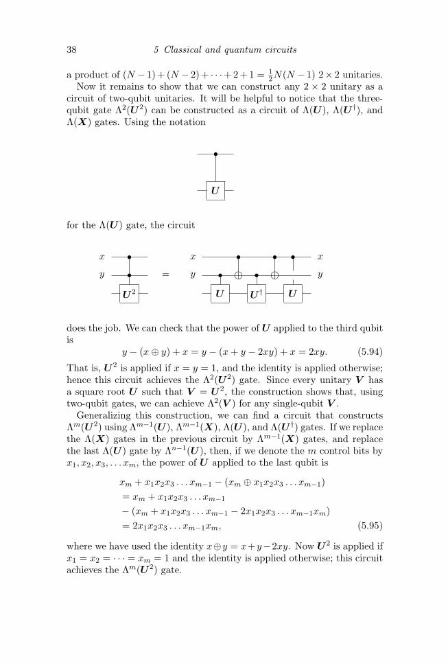
38 5 Classical and quantum circuits
a product of (N − 1)+ (N − 2)+ · · ·+2+1 = 12N(N − 1) 2× 2 unitaries.
Now it remains to show that we can construct any 2 × 2 unitary as acircuit of two-qubit unitaries. It will be helpful to notice that the three-qubit gate Λ2(U2) can be constructed as a circuit of Λ(U), Λ(U †), andΛ(X) gates. Using the notation
U
s
for the Λ(U) gate, the circuit
x
y
x
y
x
y
ssU2
= sU
sg sU †
sg sU
does the job. We can check that the power of U applied to the third qubitis
y − (x⊕ y) + x = y − (x+ y − 2xy) + x = 2xy. (5.94)
That is, U2 is applied if x = y = 1, and the identity is applied otherwise;hence this circuit achieves the Λ2(U2) gate. Since every unitary V hasa square root U such that V = U2, the construction shows that, usingtwo-qubit gates, we can achieve Λ2(V ) for any single-qubit V .
Generalizing this construction, we can find a circuit that constructsΛm(U2) using Λm−1(U), Λm−1(X), Λ(U), and Λ(U †) gates. If we replacethe Λ(X) gates in the previous circuit by Λm−1(X) gates, and replacethe last Λ(U) gate by Λn−1(U), then, if we denote the m control bits byx1, x2, x3, . . . xm, the power of U applied to the last qubit is
xm + x1x2x3 . . . xm−1 − (xm ⊕ x1x2x3 . . . xm−1)= xm + x1x2x3 . . . xm−1
− (xm + x1x2x3 . . . xm−1 − 2x1x2x3 . . . xm−1xm)= 2x1x2x3 . . . xm−1xm, (5.95)
where we have used the identity x⊕y = x+y−2xy. Now U2 is applied ifx1 = x2 = · · · = xm = 1 and the identity is applied otherwise; this circuitachieves the Λm(U2) gate.
5.4 Universal quantum gates 39
Using the construction recursively, we see that with two-qubit gateswe can construct Λ2(V ) for any V , then with these gates and two-qubitgates we can construct Λ3(V ) for any V , which allows us to constructΛ4(V ) for any V and so on. We have shown, therefore, how to constructthe n-qubit gate Λn−1(V ) for any V using a circuit of two-qubit gates.
To complete the argument showing that any element of U(2n) is aproduct of two-qubit unitaries, it will suffice to show that arbitrary 2× 2unitaries can be constructed from Λn−1(V ) and two-qubit gates. Notethat Λn−1(V ) is, in fact, a 2 × 2 unitary — it applies V in the two-dimensional space spanned by the two computational basis states
|111 . . . 110〉 , |111 . . . 111〉 . (5.96)
If we wish to apply V in the space spanned by computational states|x〉, |y〉 instead, we can use a permutation Σ of the computational basisstates with the action
Σ : |x〉 7→ |111 . . . 110〉 ,|y〉 7→ |111 . . . 111〉 , (5.97)
constructingΣ−1 Λn−1(V ) Σ . (5.98)
This is to be read from right to left, with Σ acting first and Σ−1 actinglast. But we have already seen in §5.2.2 how to construct an arbitrary per-mutation of computational basis states using Λn−1(X) gates and (single-qubit) NOT gates, and we now know how to construct Λn−1(X) (a specialcase of Λn−1(U)) from two-qubit gates. Therefore, using two-qubit gates,we have constructed the general 2× 2 unitary (in the computational ba-sis) as in eq.(5.98). That completes the proof that any element of U(2n)can be achieved by a circuit of two-qubit gates. In fact we have proven asomewhat stronger result: that the two-qubit gates Λ(U), where U isan arbitrary single-qubit gate, constitute an exactly universal gate set.
5.4.3 Finite universal gate sets
Denseness on the circle. A finite gate set is universal if circuits con-structed using that gate set are dense in U(2n). As a first simple exampleof denseness, consider the group U(1) of rotations of the circle, e.g. therotations of the Bloch sphere about the z axis:
U(θ) = exp(iθ
2σ3
), θ ∈ [0, 4π)
. (5.99)

40 5 Classical and quantum circuits
We claim that the positive integer powers of U(4πα) are dense in U(1) ifα ∈ [0, 1) is irrational. Equivalently, the points
nα (mod 1), n = 1, 2, 3, . . . , (5.100)
are dense in the unit interval.To see why, first note that the points nα (mod 1) are all distinct,
since nα = mα + k for integers k and n 6= m would imply that α is arational number α = k/(n−m). Now consider open intervals of width εcentered on each of the N points nα (mod 1), n = 1, 2, 3, . . . , N. ForNε > 1, at least two of these intervals must intersect — if all intervalswere disjoint then their total length Nε would exceed the length of theinterval. Hence there exist distinct positive integers n and m less than1/ε such that |n−m|α (mod 1) < ε; in other words, the positive integerr = |n − m| < 1/ε satisfies rα (mod 1) < ε. Now the positive integermultiples of rα (mod 1) are equally spaced points on the unit intervalseparated by less than ε. Therefore, for sufficiently large M , the intervalsof width ε centered on the points krα (mod 1), k = 1, 2, 3, . . . ,M fillthe unit interval. Since ε can be any positive real number, we concludethat the points nα (mod 1), n = 1, 2, 3, . . . are dense in the interval.
Powers of a generic gate. Generalizing this argument, consider thepositive integer powers of a generic element of U(N). In a suitable basis,U ∈ U(N) is diagonal, with eigenvalues
eiθ1/2, eiθ2/2, . . . , eiθN/2. (5.101)
Since rational numbers are countable and real numbers are not, for ageneric U (that is, for all elements of U(N) except for a set of measurezero) each θi/π and θi/θj is an irrational number. For each positive integerk, the eigenvalues e−ikθi/2, i = 1, 2, . . . , N of Uk define a point on theN -dimensional torus (the product of N circles), and as k ranges over allpositive integers, these points densely fill the whole N -torus. We concludethat for any generic U , the elements Uk, k = 1, 2, 3, . . . are dense inthe group U(1)N , i.e., come as close as we please to every unitary matrixwhich is diagonal in the same basis as U .
Note that this argument does not provide any upper bound on howlarge k must be for Uk to be ε-close to any specified element of U(1)N .In fact, the required value of k could be extremely large if, for some mand i, |mθi (mod 4π)| << ε. It might be hard (that is, require manygates) to approximate a specified unitary transformation with circuits ofcommuting quantum gates, because the unitary achieved by the circuitonly depends on how many times each gate is applied, not on the orderin which the gates are applied. It is much easier (requires fewer gates)to achieve a good approximation using circuits of noncommuting gates.
5.4 Universal quantum gates 41
If the gates are noncommuting, then the order in which the gates areapplied matters, and many more unitaries can be reached by circuits ofspecified size than if the gates are noncommuting.
Reaching the full Lie algebra. Suppose we can construct the two gatesU = exp (iA) ,V = exp (iB) ∈ U(N), where A and B are N × NHermitian matrices. If these are generic gates, positive powers of U comeas close as we please to eiαA for any real α and positive powers of V comeas close as we please to eiβB for any real β. That is enough to ensurethat there is a finite circuit constructed from U and V gates that comesas close as we please to eiC , where C is any Hermitian element of the Liealgebra generated by A and B.
We say that a unitary transformation U is reachable if for any ε > 0there is a finite circuit achieving U which is ε-close to U in the sup norm.Noting that
limn→∞
(eiαA/neiβB/n)n = limn→∞
(1 +
i
n(αA + βB) +O
(1n2
))n
= ei(αA+βB), (5.102)
we see that any ei(αA+βB) is reachable if each eiαA/n and eiβB/n is reach-able. Furthermore, because
limn→∞
(eiA/
√neiB/
√ne−iA/
√ne−iB/
√n)n
= limn→∞
(1− 1
n(AB −BA) +O
(1
n3/2
))n
= e−[A,B], (5.103)
we see that e−[A,B] is also reachable.For example, positive integer powers of a generic element of SU(2) allow
us to reach a U(1) subgroup; if we orient our axes on the Bloch sphereappropriately, this is the subgroup generated by the Pauli operator Z.Positive integer powers of a second generic element of SU(2) allow us toreach a different U(1) subgroup, generated by X = X + γZ (for somereal γ) with an appropriate choice of axes. Because [Z,X] = iY , theelements Z, X,−i[Z, X] span the three-dimensional SU(2) Lie algebra.It follows that circuits built from any two generic elements of SU(2) sufficeto reach any element of SU(2).
This observation applies to higher-dimensional Lie algebras as well.For example, the SU(4) Lie algebra is 15 dimensional. It contains variouslower-dimensional subalgebras, such as the Lie algebras of the SU(4) sub-groups U(1)3, SU(2)×SU(2)×U(1), SU(3)×U(1), etc. But two genericelements of the SU(4) Lie algebra already suffice to general the full Liealgebra. The generated algebra closes on one of the lower-dimensional

42 5 Classical and quantum circuits
subalgebras only if some nested commutators vanish “by accident,” a cri-terion satisfied by only a set of measure zero among all pairs of SU(4)generators. Actually, as we have already noted, a generic element ofSU(4) allows us to reach the torus U(1)3, and no nontrivial subgroupof SU(4) contains two generic U(1)3 subgroups. Therefore, circuits builtfrom two generic two-qubit gates suffice to reach any two-qubit gate (upto an overall phase). And since we can reach any element of U(2n) withtwo-qubit gates, a pair of generic two-qubit gates provides a universalgate set, assuming we can apply the gates to any pair of qubits.
But in fact just one generic two-qubit gate is already enough, if we arefree to choose not just the pair of qubits on which the gate acts but alsothe ordering of the qubits. That is, a generic two-qubit gate does notcommute with the operator SWAP which interchanges the two qubits.If U is a generic two-qubit gate, then
V = SWAP U SWAP (5.104)
(the same gate applied to the same two qubits, but in the opposite order)is another two-qubit gate not commuting with U . Positive powers of Ureach one U(1)3 subgroup of SU(4) while positive powers of V reach adifferent U(1)3, so that circuits built from U and V reach all of SU(4).
Even nongeneric universal gates, in particular gates whose eigenvaluesare all rational multiples of π, can suffice for universality. One examplediscussed in the homework is the gate set CNOT,H,T , where H ro-tates the Bloch sphere by the angle π about the axis 1√
2(x+ x), and T
rotates the Bloch sphere by the angle π/4 about the z axis. If we replacedT with the π/2 rotation T 2, then the gate set would not be universal; inthat case the only achievable single-qubit rotations would be those in afinite subgroup of SU(2), the symmetry group of the cube. But SU(2)has few such finite nonabelian subgroups (the only finite nonabelian sub-groups of the rotation group SO(3) are the symmetry groups of regularpolygons and of regular three-dimensional polyhedra, the platonic solids).If the gate set reaches beyond these finite subgroups it will reach either aU(1) subgroup of SU(2) or all of SU(2).
5.4.4 The Solovay-Kitaev approximation
Up until now our discussion of universal gates has focused on reachabilityand has ignored complexity. But when we have a finite universal gateset, we want to know not only whether we can approximate a desiredunitary transformation to accuracy ε, but also how hard it is to achievethat approximation. How large a circuit suffices? The question really hastwo parts. (1) Given a unitary transformation U , how large a quantum
5.4 Universal quantum gates 43
circuit is needed to construct U such that ‖U − eiφU‖sup ≤ ε? (2) Howlarge a classical circuit is needed to find the quantum circuit that achievesU? We will see that, for any universal set of gates (closed under inverse)used to approximate elements of a unitary group of constant dimension,the answer to both questions is polylog(1/ε). We care about the answerto the second question because it would not be very useful to know thatU can be well approximated by small quantum circuits if these circuitsare very hard to find.
We will prove this result by devising a recursive algorithm whichachieves successively better and better approximations. We say that afinite repertoire of unitary transformations R is an “ε-net” in U(N) ifevery element of U(N) is no more than distance ε away (in the sup norm)from some element of R, and we say that R is “closed under inverse” ifthe inverse of every element of R is also in R. The key step of the recur-sive algorithm is to show that if R is an ε-net, closed under inverse, thenwe can construct a new repertoire R′, also closed under inverse, with thefollowing properties: (1) each element of R′ is achieved by a circuit of atmost 5 gates from R. (2) R′ is an ε′-net, where
ε′ = Cε3/2 , (5.105)
and C is a constant.Before explaining how this step works, let’s see why it ensures that we
can approximate any unitary using a quantum circuit with size polylog-arithmic in the accuracy. Suppose to start with that we have found anε0-net R0, closed under inverse, where each element of R0 can be achievedby a circuit with no more than L0 gates chosen from our universal gateset. If ε0 < 1/C2, then we can invoke the recursive step to find an ε1-netR1, where ε1 < ε0, and each element of R1 can be achieved by a circuitof L1 = 5L0 gates. By repeating this step k times, we can make the errorεk much smaller than the level-0 error ε0. Iterating the relation
C2εk =(C2εk−1
)3/2 (5.106)
k times we obtain
C2εk =(C2ε0
)(3/2)k
, (5.107)
and by taking logs of both sides we find(32
)k
=log(1/C2εk
)log (1/C2ε0)
. (5.108)
After k recursive steps the circuit size for each unitary in the εk-net Rk

44 5 Classical and quantum circuits
is no larger than Lk where
Lk/L0 = 5k =
((32
)k)log 5/ log(3/2)
=
(log(1/C2εk
)log (1/C2ε0)
)log 5/ log(3/2)
.
(5.109)
Thus the circuit size scales with the accuracy εk as [log(1/εk)]3.97.
Now let’s see how the ε′-net R′ is constructed from the ε-net R. Forany U ∈ SU(N) there is an element U ∈ R such that ‖U − U‖sup ≤ ε,or equivalently ‖UU
−1 − I‖sup ≤ ε. Now we will find W , constructedas a circuit of 4 elements of R, such that ‖UU
−1 − W |sup ≤ ε′, orequivalently ‖U −WU |sup ≤ ε′. Thus U is approximated to accuracy ε′
by WU , which is achieved by a circuit of 5 elements of R.We may write UU
−1= eiA, where A = O(ε). (By A = O(ε) we mean
‖A‖sup = O(ε), i.e., ‖A‖sup is bounded above by a constant times ε for εsufficiently small. ) It is possible to find Hermitian B, C, both O(ε1/2),such that [B,C] = −iA. Furthermore, because R is an ε-net, there is anelement eiB of R which is ε-close to eiB, and an element eiC of R whichis ε-close to eiC . It follows that B − B = O(ε) and C − C = O(ε).
Now we consider the circuit
W = eiBeiCe−iBe−iC = I − [B, C] +O(ε3/2); (5.110)
the remainder term is cubic order in B and C, hence O(ε3/2). First notethat the inverse of this circuit, eiCeiBe−iCe−iB, can also be constructedas a size-4 circuit of gates from R. Furthermore,
W = I − [B +O(ε),C +O(ε)] +O(ε3/2) = I + iA +O(ε3/2)
= eiA +O(ε3/2); (5.111)
thus W , a circuit of 4 gates from R, approximates UU−1
to O(ε3/2)accuracy, as we wanted to show.
Finally, let’s consider the classical computational cost of finding thequantum circuit which approximates a unitary transformation. The clas-sical algorithm receives a unitary transformation U as input, and pro-duces as output a quantum circuit evaluating U , which approximates Uto accuracy ε. To improve the accuracy of the approximation to ε′, weneed to call the accuracy-ε algorithm three times, to find circuits evalu-ating U , eiB, and eiC . Therefore, if the classical cost of the accuracy-εalgorithm is t, the classical cost of the improved accuracy-ε′ algorithm ist′ = 3t+constant, where the additive constant is needed to cover the cost
5.5 Summary 45
of tasks that do not scale with ε, such as finding the matrices B and Csatisfying [B,C] = −iA. After k iterations, the classical cost scales like
O(3k) = O([log(1/εk)]
log 3/ log(3/2))
= O([log(1/εk)]
2.71), (5.112)
polylogarithmic in the accuracy achieved by the level-k version of thealgorithm.
What we have accomplished is a bit surprising. By composing unitarytransformations with O(ε) errors we have obtained unitary transforma-tions with smaller O(ε3/2) errors. How could we achieve such sharp resultswith such blunt tools? The secret is that we have constructed our circuitso that the O(ε) errors cancel, leaving only the higher-order errors. Thiswould not have worked if R had not been closed under inverse. If insteadof the inverses of eiB and eiC we had been forced to use O(ε) approxima-tions to these inverses, the cancellations would not have occurred, and ourquest for an improved approximation would have failed. But if our uni-versal gate set allows us to construct the exact inverse of each element ofthe gate set, then we can use the Solovay-Kitaev approach to recursivelyimprove the approximation.
This scheme works for any universal gate set that is closed under in-verse. For particular gate sets improved approximations are possible. Forexample, the gate set H,T can be used to approximate an arbitrarysingle-qubit unitary to accuracy ε using O(log(1/ε)) gates, a substantialimprovement over O([log(1/ε)]3.97) established by the general argument,and the circuits achieving this improved overhead cost can be efficientlyconstructed.
5.5 Summary
Classical circuits. The complexity of a problem can be characterizedby the size of a uniform family of logic circuits that solve the problem:The problem is hard if the size of the circuit is a superpolynomial func-tion of the size of the input, and easy otherwise. One classical universalcomputer can simulate another efficiently, so the classification of com-plexity is machine independent. The 3-bit Toffoli gate is universal forclassical reversible computation. A reversible computer can simulate anirreversible computer without a significant slowdown and without unrea-sonable memory resources.
Quantum Circuits. Although there is no proof, it seems likelythat polynomial-size quantum circuits cannot be simulated in generalby polynomial-size randomized classical circuits (BQP 6= BPP); however,polynomial space is sufficient (BQP ⊆ PSPACE). A noisy quantum circuitcan simulate an ideal quantum circuit of size T to acceptable accuracy

46 5 Classical and quantum circuits
if each quantum gate has an accuracy of order 1/T . Any n-qubit uni-tary transformation can be constructed from two-qubit gates. A generictwo-qubit quantum gate, if it can act on any two qubits in a device, issufficient for universal quantum computation. One universal quantumcomputer can simulate another to accuracy ε with a polylog(1/ε) over-heard cost; therefore the complexity class BQP is machine independent.
Do the Exercises to learn more about universal sets of quantum gates.
5.6 Exercises
5.1 Linear simulation of Toffoli gate.
In §5.2.2 we constructed the n-bit Toffoli gate Λn−1(X) from 3-bitToffoli gates (Λ2(X)’s). The circuit required only one bit of scratchspace, but the number of gates was exponential in n. With morescratch, we can substantially reduce the number of gates.
a) Find a circuit family with 2n − 5 Λ2(X)’s that evaluatesΛn−1(X). (Here n − 3 scratch bits are used, which are setto 0 at the beginning of the computation and return to thevalue 0 at the end.)
b) Find a circuit family with 4n − 12 Λ2(X)’s that evaluatesΛn−1(X), which works irrespective of the initial values of thescratch bits. (Again the n−3 scratch bits return to their initialvalues, but they don’t need to be set to zero at the beginning.)
5.2 An exactly universal quantum gate set.
The purpose of this exercise is to complete the demonstration thatthe controlled-NOT gate Λ(X) and arbitrary single-qubit gates con-stitute an exactly universal set.
a) If U is any unitary 2 × 2 matrix with determinant one, findunitary A,B, and C such that
ABC = I (5.113)
AXBXC = U . (5.114)
Hint: From the Euler angle construction, we know that
U = Rz(ψ)Ry(θ)Rz(φ), (5.115)
where, e.g., Rz(φ) denotes a rotation about the z-axis by theangle φ. We also know that, e.g.,
XRz(φ)X = Rz(−φ). (5.116)

5.6 Exercises 47
b) Consider a two-qubit controlled phase gate which applies U =eiα1 to the second qubit if the first qubit has value |1〉, andacts trivially otherwise. Show that it is actually a one-qubitgate.
c) Draw a circuit using Λ(X) gates and single-qubit gates that im-plements Λ(U), where U is an arbitrary 2 × 2 unitary trans-formation.
Since the argument in §5.4.2 shows that the gate set Λ(U) isexactly universal, we have shown that Λ(X) together with single-qubit gates are an exactly universal set.
5.3 Universal quantum gates I
In this exercise and the two that follow, we will establish that severalsimple sets of gates are universal for quantum computation.
The Hadamard transformation H is the single-qubit gate that actsin the standard basis |0〉, |1〉 as
H =1√2
(1 11 −1
); (5.117)
in quantum circuit notation, we denote the Hadamard gate as
H
The single-qubit phase gate S acts in the standard basis as
S =(
1 00 i
), (5.118)
and is denoted
S
A two-qubit controlled phase gate Λ(S) acts in the standard basis|00〉, 01〉, |10〉, |11〉 as the diagonal 4× 4 matrix
Λ(S) = diag(1, 1, 1, i) (5.119)
and can be denoted
S
s
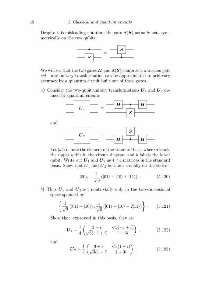
48 5 Classical and quantum circuits
Despite this misleading notation, the gate Λ(S) actually acts sym-metrically on the two qubits:
S
s=
SsWe will see that the two gates H and Λ(S) comprise a universal gateset – any unitary transformation can be approximated to arbitraryaccuracy by a quantum circuit built out of these gates.
a) Consider the two-qubit unitary transformations U1 and U2 de-fined by quantum circuits
U1 =H s
S
H
and
U2 =H sS H
Let |ab〉 denote the element of the standard basis where a labelsthe upper qubit in the circuit diagram and b labels the lowerqubit. Write out U1 and U2 as 4× 4 matrices in the standardbasis. Show that U1 and U2 both act trivially on the states
|00〉, 1√3
(|01〉+ |10〉+ |11〉) . (5.120)
b) Thus U1 and U2 act nontrivially only in the two-dimensionalspace spanned by
1√2
(|01〉 − |10〉) , 1√6
(|01〉+ |10〉 − 2|11〉). (5.121)
Show that, expressed in this basis, they are
U1 =14
(3 + i
√3(−1 + i)√
3(−1 + i) 1 + 3i
), (5.122)
and
U2 =14
(3 + i
√3(1− i)√
3(1− i) 1 + 3i
). (5.123)
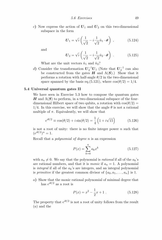
5.6 Exercises 49
c) Now express the action of U1 and U2 on this two-dimensionalsubspace in the form
U1 =√i
(1√2− i
1√2n1 · ~σ
), (5.124)
and
U2 =√i
(1√2− i
1√2n2 · ~σ
). (5.125)
What are the unit vectors n1 and n2?
d) Consider the transformation U−12 U1 (Note that U−1
2 can alsobe constructed from the gates H and Λ(S).) Show that itperforms a rotation with half-angle θ/2 in the two-dimensionalspace spanned by the basis eq.(5.121), where cos(θ/2) = 1/4.
5.4 Universal quantum gates II
We have seen in Exercise 5.3 how to compose the quantum gatesH and Λ(S) to perform, in a two-dimensional subspace of the four-dimensional Hilbert space of two qubits, a rotation with cos(θ/2) =1/4. In this exercise, we will show that the angle θ is not a rationalmultiple of π. Equivalently, we will show that
eiθ/2 ≡ cos(θ/2) + i sin(θ/2) =14
(1 + i
√15)
(5.126)
is not a root of unity: there is no finite integer power n such that(eiθ/2)n = 1.
Recall that a polynomial of degree n is an expression
P (x) =n∑
k=0
akxk (5.127)
with an 6= 0. We say that the polynomial is rational if all of the ak’sare rational numbers, and that it is monic if an = 1. A polynomialis integral if all of the ak’s are integers, and an integral polynomialis primitive if the greatest common divisor of a0, a1, . . . , an is 1.
a) Show that the monic rational polynomial of minimal degree thathas eiθ/2 as a root is
P (x) = x2 − 12x+ 1 . (5.128)
The property that eiθ/2 is not a root of unity follows from the result(a) and the
50 5 Classical and quantum circuits
Theorem If a is a root of unity, and P (x) is a monic rationalpolynomial of minimal degree with P (a) = 0, then P (x) is integral.
Since the minimal monic rational polynomial with root eiθ/2 is notintegral, we conclude that eiθ/2 is not a root of unity. In the rest ofthis exercise, we will prove the theorem.
b) By “long division” we can prove that if A(x) and B(x) are ra-tional polynomials, then there exist rational polynomials Q(x)and R(x) such that
A(x) = B(x)Q(x) +R(x) , (5.129)
where the “remainder” R(x) has degree less than the degreeof B(x). Suppose that an = 1, and that P (x) is a rationalpolynomial of minimal degree such that P (a) = 0. Show thatthere is a rational polynomial Q(x) such that
xn − 1 = P (x)Q(x) . (5.130)
c) Show that if A(x) and B(x) are both primitive integral polyno-mials, then so is their product C(x) = A(x)B(x). Hint: IfC(x) =
∑k ckx
k is not primitive, then there is a prime num-ber p that divides all of the ck’s. Write A(x) =
∑l alx
l, andB(x) =
∑m bmx
m, let ar denote the coefficient of lowest orderin A(x) that is not divisible by p (which must exist if A(x) isprimitive), and let bs denote the coefficient of lowest order inB(x) that is not divisible by p. Express the product arbs interms of cr+s and the other al’s and bm’s, and reach a contra-diction.
d) Suppose that a monic integral polynomial P (x) can be factoredinto a product of two monic rational polynomials, P (x) =A(x)B(x). Show that A(x) and B(x) are integral. Hint:First note that we may write A(x) = (1/r) · A(x), andB(x) = (1/s) · B(x), where r, s are positive integers, and A(x)and B(x) are primitive integral; then use (c) to show thatr = s = 1.
e) Combining (b) and (d), prove the theorem.
What have we shown? Since U−12 U1 is a rotation by an irrational
multiple of π, the powers of U−12 U1 are dense in a U(1) subgroup.
Similar reasoning shows that U1U−12 is a rotation by the same angle
about a different axis, and therefore its powers are dense in anotherU(1) subgroup. Products of elements of these two noncommuting
5.6 Exercises 51
U(1) subgroups are dense in the SU(2) subgroup that contains bothU1 and U2.
Furthermore, products of
Λ(S)U−12 U1Λ(S)−1 and Λ(S)U1U
−12 Λ(S)−1 (5.131)
are dense in another SU(2), acting on the span of1√2(|01〉 − |10〉), 1√
6(|01〉+ |10〉 − 2i|11〉)
. (5.132)
Together, these two SU(2) subgroups close on the SU(3) subgroupthat acts on the three-dimensional space orthogonal to |00〉. Con-jugating this SU(3) by H ⊗ H we obtain another SU(3) act-ing on the three-dimensional space orthogonal to |+,+〉, where|+〉 = 1√
2(|0〉 + |1〉). The only subgroup of SU(4) that contains
both of these SU(3) subgroups is SU(4) itself.
Therefore, the circuits constructed from the gate set H,Λ(S)are dense in SU(4) — we can approximate any two-qubit gate toarbitrary accuracy, which we know suffices for universal quantumcomputation. Whew!
5.5 Universal quantum gates III
We have shown in Exercises 5.3 and 5.4 that the gate set H,Λ(S)is universal. Thus any gate set from which both H and Λ(S) canbe constructed is also universal. In particular, we can see thatH,S,Λ2(X) and H,T ,Λ(X) are universal gates sets, whereT = exp
(−iπ8 Z
).
a) It is sometimes convenient to characterize a quantum gate byspecifying the action of the gate when it conjugates a Paulioperator. Show that H and S have the properties
HXH = Z , HY H = −Y , HZH = X , (5.133)
and
SXS−1 = Y , SY S−1 = −X , SZS−1 = Z . (5.134)
b) Note that, since S−1 = S3, the gate K = HS−1HSH can beconstructed using H and S. Show that
KXK = Y , KY K = X , KZK = −Z . (5.135)

52 5 Classical and quantum circuits
c) Construct circuits for Λ2(Y ) and Λ2(Z) using the gate setH,S,Λ2(X). Then complete the proof of universality forthis gate set by constructing Λ(S) ⊗ I using Λ2(X), Λ2(Y ),and Λ2(Z).
d) Show that H,T ,Λ(X) is a universal gate set by constructinga circuit for Λ(S) from Λ(X) and T . Hint: Observe thatT 2 = e−iπ/4S, then use the construction suggested in Exercise5.2, noting that T−1T−1T 2 = I and T−1XT−1XT 2 = T 2.
The Toffoli gate Λ2(X) is universal for reversible classical compu-tation. What must be added to realize the full power of quantumcomputing? We have just seen that the single-qubit gates H and S,together with the Toffoli gate, are adequate for reaching any unitarytransformation. But in fact, just H and Λ2(X) suffice to efficientlysimulate any quantum computation.
Of course, since H and Λ2(X) are both real orthogonal matrices,a circuit composed from these gates is necessarily real — there arecomplex n-qubit unitaries that cannot be constructed with thesetools. But a 2n-dimensional complex vector space is isomorphic toa 2n+1–dimensional real vector space. A complex vector can beencoded by a real vector according to
|ψ〉 =∑
x
ψx|x〉 7→ |ψ〉 =∑
x
(Re ψx)|x, 0〉+(Im ψx)|x, 1〉 , (5.136)
and the action of the unitary transformation U can be representedby a real orthogonal matrix UR defined as
UR : |x, 0〉 7→ (Re U)|x〉 ⊗ |0〉+ (Im U)|x〉 ⊗ |1〉 ,|x, 1〉 7→ −(Im U)|x〉 ⊗ |0〉+ (Re U)|x〉 ⊗ |1〉 .(5.137)
To show that the gate set H,Λ2(X) is “universal,” it sufficesto demonstrate that the real encoding Λ(S)R of Λ(S) can be con-structed from Λ2(X) and H.
d) Verify that Λ(S)R = Λ2(XZ).
e) Use Λ2(X) and H to construct a circuit for Λ2(XZ).
Thus, the classical Toffoli gate does not need much help to unleashthe power of quantum computing. In fact, any nonclassical single-qubit gate (one that does not preserve the computational basis),combined with the Toffoli gate, is sufficient.
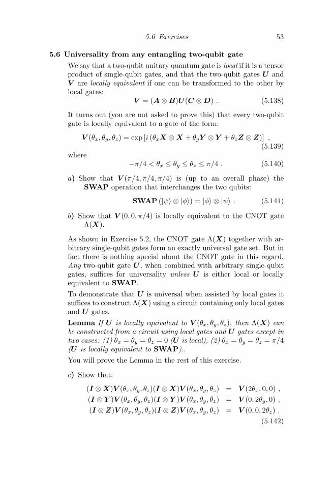
5.6 Exercises 53
5.6 Universality from any entangling two-qubit gate
We say that a two-qubit unitary quantum gate is local if it is a tensorproduct of single-qubit gates, and that the two-qubit gates U andV are locally equivalent if one can be transformed to the other bylocal gates:
V = (A⊗B)U(C ⊗D) . (5.138)
It turns out (you are not asked to prove this) that every two-qubitgate is locally equivalent to a gate of the form:
V (θx, θy, θz) = exp [i (θxX ⊗X + θyY ⊗ Y + θzZ ⊗Z)] ,(5.139)
where−π/4 < θx ≤ θy ≤ θz ≤ π/4 . (5.140)
a) Show that V (π/4, π/4, π/4) is (up to an overall phase) theSWAP operation that interchanges the two qubits:
SWAP (|ψ〉 ⊗ |φ〉) = |φ〉 ⊗ |ψ〉 . (5.141)
b) Show that V (0, 0, π/4) is locally equivalent to the CNOT gateΛ(X).
As shown in Exercise 5.2, the CNOT gate Λ(X) together with ar-bitrary single-qubit gates form an exactly universal gate set. But infact there is nothing special about the CNOT gate in this regard.Any two-qubit gate U , when combined with arbitrary single-qubitgates, suffices for universality unless U is either local or locallyequivalent to SWAP.To demonstrate that U is universal when assisted by local gates itsuffices to construct Λ(X) using a circuit containing only local gatesand U gates.Lemma If U is locally equivalent to V (θx, θy, θz), then Λ(X) canbe constructed from a circuit using local gates and U gates except intwo cases: (1) θx = θy = θz = 0 (U is local), (2) θx = θy = θz = π/4(U is locally equivalent to SWAP)..You will prove the Lemma in the rest of this exercise.
c) Show that:
(I ⊗X)V (θx, θy, θz)(I ⊗X)V (θx, θy, θz) = V (2θx, 0, 0) ,(I ⊗ Y )V (θx, θy, θz)(I ⊗ Y )V (θx, θy, θz) = V (0, 2θy, 0) ,(I ⊗Z)V (θx, θy, θz)(I ⊗Z)V (θx, θy, θz) = V (0, 0, 2θz) .
(5.142)
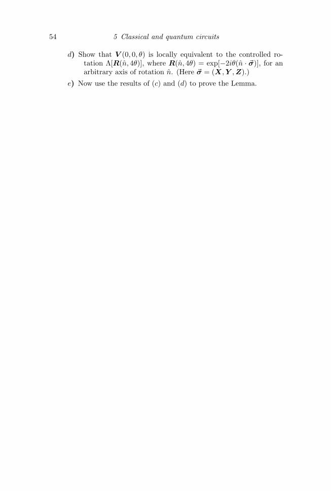
54 5 Classical and quantum circuits
d) Show that V (0, 0, θ) is locally equivalent to the controlled ro-tation Λ[R(n, 4θ)], where R(n, 4θ) = exp[−2iθ(n · ~σ)], for anarbitrary axis of rotation n. (Here ~σ = (X,Y ,Z).)
e) Now use the results of (c) and (d) to prove the Lemma.