Lecture notes for Math 61CM, Linear algebra, Version 2018

Lenya Ryzhik∗

October 14, 2018

Nothing found here is original except for a few mistakes and misprints here and there. Thesenotes are simply a record of what I cover in class, to spare the students some of the necessity oftaking the lecture notes and compensate for my bad handwriting. The material comes mostly fromthe book Leon Simon ”An Introduction to Multivariable Mathematics” and lecture notes by AndrasVasy.

1 Notes on algebra

This section goes a little bit more generally about the notion of a field we have introduced in theanalysis class when we defined the axioms for the real numbers. We start with the definition of agroup.

Definition 1.1 A group (G, ∗) is a set G together with a map ∗ : G×G→ G with the properties

1. (Associativity) For all x, y, z ∈ G, x ∗ (y ∗ z) = (x ∗ y) ∗ z.

2. (Units) There exists e ∈ G such that for all x ∈ G, x ∗ e = x = e ∗ x.

3. (Inverses) For all x ∈ G there exists y ∈ G such that x ∗ y = e = y ∗ x.

A basic property is that one can talk about the unit, that is, given (1) and (2), e is unique:

Lemma 1.2 In any group (G, ∗), the unit e is unique.

Proof: Suppose e, f ∈ G are units. Then e = e ∗ f since f is a unit, and e ∗ f = f since e is aunit. Combining these, e = f . �

Note that this proof used only (1) and (2), so it is useful to define a more general notion thanthat of a group.

Definition 1.3 A semigroup (G, ∗) is a set G together with a map ∗ : G×G→ G with the properties

1. (Associativity) For all x, y, z ∈ G, x ∗ (y ∗ z) = (x ∗ y) ∗ z.

2. (Units) There exists e ∈ G such that for all x ∈ G, x ∗ e = x = e ∗ x.

Thus, a semigroup would be a group if each element had an inverse. Notice also that the proofof the above lemma shows that even in a semigroup, the unit is unique.

Inverses are also unique in a group, or, when they exist, in a semigroup.

∗Department of Mathematics, Stanford University, Stanford, CA 94305, USA; ryzhik@math.stanford.edu

1

Lemma 1.4 Suppose that (G, ∗) is a semigroup with unit e, x ∈ G, and suppose that there existy, z ∈ G such that y ∗ x = e = x ∗ z. Then y = z.

Notice that if G is a group, the existence of such a y, z is guaranteed, even with y = z, by (3).Thus, this lemma says in particular that in a group, inverses are unique.

However, it says more: in a semigroup, any left inverse (if it exists) equals any right inverse (ifit exists). In particular, if both left and right inverses exist, they are both unique: e.g. if y, y′ areleft inverses, they are both equal to any left inverse z, and thus to each other.

Proof: We havey = y ∗ e = y ∗ (x ∗ z),

where we used that e is the unit and x ∗ z = e. Similarly, we have

z = e ∗ z = (y ∗ x) ∗ z.

But by the associativity, y ∗ (x∗z) = (y ∗x)∗z, so combining these three equations shows that z = y,as desired. �

There are many interesting groups, such as (R,+), (Z,+), (Q,+), (Rn,+), (R+, ·), where R+

consists of the positive reals, as well as semigroups, such as (R, ·) (all non-zero elements have inverses),(Z, ·) (only ±1 have inverses). Another group with a different flavor is (Zn,+), the integers modulon ≥ 2 integer: as a set, this can be identified with {0, 1, . . . , n − 1} (the remainders when dividingby n), and addition gives the usual sum in Z, reduced modulo n, For instance, in (Z5,+), we have2 + 4 = 1. It may be less confusing though to write {[0], . . . , [n− 1]} for the set, and represent thelast identity in Z5 as [2] + [4] = [1]. In general, when the operation is understood, one might justwrite the set for a group or semigroup, without indicating the operation.

An important and slightly different class of groups are groups of transformations. Fix a set Xand consider maps G : X → X with composition serving as group multiplication: G1 ◦G2 is a mapfrom X to X such that G1 ◦G2(x) = G1(G2(x)). A collection G of such maps forms a group if (1) itis closed under composition: if G1, G2 ∈ G then G1 ◦ G2 ∈ G, (2) the identity map Id is in G –recall that Id(x) = x for all x ∈ X, and (3) for each G ∈ G there is a map G−1 in G such thatG ◦G−1 = G−1 ◦G = Id.

Exercise 1.5 Show that a map G : X → X has a left-and-right inverse G−1 such that G ◦ G−1 =G−1 ◦G = Id if and only if G is one-to-one and onto.

Exercise 1.6 Show that the maps R2 → R2 of the form (x1, x2) → (ax1 + bx2, cx2 + dx2) withad− bc = 1 form group.

Exercise 1.7 Let `∞ be the set of all infinite sequences a = (a1, a2, . . . , an, . . . ) such that thereexists a constant M that depends on the sequence but not on n so that

|an| ≤M for all n ∈ N.

Define a map Sk acting on such sequences as Sk : `∞ → `∞ as Ska = b, with the sequence bn havingthe entries

bn = e−kan.

Show that each Sk maps `∞ to `∞. In other words, that if the sequence an is in `∞, then thesequence bn is also in `∞, and also show that Sk, k ∈ Z form a group, with Id = S0, and Sk ◦ Sn =Sk+n.

2

An example of a semi-group that may be less familiar is as follows. Again, let `∞ be the set of allinfinite sequences a = (a1, a2, . . . , an, . . . ) such that there exists a constant M that depends on thesequence but not on n so that

|an| ≤M for all n ∈ N.

Given any k ≥ 0, we may define a map Dk : `0 → `0 as Dka = b, with the sequence bn having theentries

bn = e−knan.

If a ∈ `∞, there exists M so that |an| ≤M for all n. Then we have

|bn| ≤ e−kn|an| ≤ e−knM ≤M,

hence the sequence bn is also in l∞. Thus, Sk is, indeed, a map from `∞ to `∞. It is also easy tocheck that the set G of all Sk, with k ≥ 0, is a commutative semi-group, with the product given bythe composition of maps:

Sk ◦ Sn = Sk+n, (1.1)

and Id = S0 being the unit.

Exercise 1.8 Check that (1.1), indeed, holds, where the left side is the composition of Sn and Sk.

However, Sk can not have an inverse in G. Indeed, if there is a map Dk that maps `∞ to `∞ suchthat Dk ◦ Sk = Id, then it would act as Dka = c, with the entries

cn = eknan.

In other words, we would have to set Dk = S−k for k ≥ 0. However, such Dk is not a map in G.Moreover, we can not add to G maps ”Sk with k < 0” if we want to keep them as maps from `∞to `∞. This is because of the following exercise.

Exercise 1.9 Fix k ∈ N and find a sequence a = (a1, a2, . . . , an, . . . ) that belongs to `∞ such thatthe sequence b = (b1, b2, . . . , bn, . . . ) with the entries

bn = eknan

does not belong to `∞.

Many (semi)groups are commutative; in fact, all of the above examples are:

Definition 1.10 A commutative, or abelian, semigroup (G, ∗) is one in which x ∗ y = y ∗ x for allx, y ∈ G.

Noncommutative semigroups will play a role in this class, including the set Mn of n×n matriceswith matrix multiplication as the operation, which is non-commutative if n ≥ 2, and permutationsof a finite set S which is non-commutative if the set has at least 3 elements (this will be discussedwhen we talk about determinants).

We then can make the following definition:

Definition 1.11 A field (F,+, ·) is a set F with two maps + : F ×F → F and · : F ×F → F suchthat

1. (F,+) is a commutative group, with unit 0.

3

2. (F, ·) is a commutative semigroup with unit 1 such that 1 6= 0 and such that x 6= 0 implies thatx has a multiplicative inverse (i.e. y such that x · y = 1 = y · x).

3. The distributive law holds:x · (y + z) = x · y + x · z.

One usually writes −x for the additive inverse (inverse with respect to +), x−1 for the multi-plicative inverse. The common examples of a field include (R,+, ·), (Q,+, ·), and complex numbers(C,+, ·). A more interesting field is the subset of R of numbers of the form

{a+ b√

2 : a, b ∈ Q}.

The most interesting part in showing that this is a field is that multiplicative inverses exist; thatthese exist (within this set!) when a+ b

√2 6= 0 follows from the following computation in R:

(a+ b√

2)−1 =a− b

√2

a2 − 2b2= (a2 − 2b2)−1a− (a2 − 2b2)−1b

√2.

Note that both (a2−2b2)−1a,−(a2−2b2)−1b are, indeed, rational, and the denominator a2−2b2 6= 0,since

√2 is an irrational number.

Finally, Zn is not a field for a general n. For instance, if n = 6, [2] · [3] = [0]. However, if n is aprime p, then it is – it is the finite field of p = n elements.

Exercise 1.12 Check that Zn is a field if and only if n is a prime number.

Another very important example is the set C of complex numbers z = x+ iy, with x, y ∈ R and therules of addition

(x+ iy) + (u+ iw) = (x+ u) + i(y + w), (1.2)

and multiplication(x+ iy)(u+ iw) = (xu− yw) + i(yu+ xw). (1.3)

Exercise 1.13 Show that C is a field, and the inverse of a complex number x+ iy is given by

(x+ iy)−1 =x

x2 + y2− i y

x2 + y2, (1.4)

provided that not both x = 0 and y = 0.

As an example of a general result in a field, let us show the following.

Lemma 1.14 If (F,+, ·) is a field, then 0 · x = 0 for all x ∈ F .

Proof. Since 0 = 0 + 0, we have

0 · x = (0 + 0) · x = 0 · x+ 0 · x, (1.5)

so

0 = −(0 · x) + (0 · x) = −(0 · x) + (0 · x+ 0 · x) = (−(0 · x) + 0 · x) + 0 · x = 0 + 0 · x = 0 · x,

as desired. On the last line, the first equality uses that −(0 · x) is the additive inverse of 0 · x, thesecond uses (1.5), the third uses associativity of addition, the fourth uses again that −(0 · x) is theadditive inverse of 0 · x, while the fifth uses that 0 is the additive unit. �

Notice that this proof uses the distributive law crucially: this is what links addition (0 is theadditive unit!) to multiplication.

For more examples, see Appendix A, Problem 1.1 in the Simon book, and the analysis lecturenotes.

4

2 Vector spaces

2.1 The definition of a vector space

One usually encounters first vectors as ”arrows” on the plane that can be added and multiplied by areal number. The general definition of a vector space generalizes this concept in a dramatic fashion.

Definition 2.1 A vector space V over a field F is a set V such that the sum v + w ∈ V is definedfor any two elements v, w ∈ V , and for λ ∈ F and v ∈ V the product λv is defined as an elementof V . These operations satisfy the following properties.

1. The set (V,+) is a commutative group, with unit 0 and with the inverse of x denoted by −x,

2. For all x ∈ V , λ, µ ∈ F, we have

(λ ? µ)x = λ(µx), 1x = x.

Here, 1 is the multiplicative unit of the field F and ? denotes the product in F. Note that inthe expression λ ? µ in the left side, we are using the field multiplication in F; everywhere elsethe product is by an element in F and in V .

3. For all x, y ∈ V , λ, µ ∈ F,(λ+ µ)x = λx+ µx

andλ(x+ y) = λx+ λy,

so that the two distributive laws hold.

Note that the two distributive laws are different: in the first, in the left side, + is in F, in the second,it is in V . In the right side, it is in V in both distributive laws.

The ‘same’ argument as for fields shows that 0x = 0, and λ0 = 0, where, in the first case, in theleft 0 is the additive unit of the field, and all other 0’s are the zero vector, the additive unit of thevector space. Another example of what one can prove in a vector space is

Lemma 2.2 Suppose V is a vector space over a field F. Then (−1)x = −x.

Proof. We have, using the distributive law, and that 0x = 0, observed above,

0 = 0x = (1 + (−1))x = 1x+ (−1)x = x+ (−1)x,

which says exactly that (−1)x is the additive inverse of x, which we denote by −x. �

Remark 2.3 In these lectures, we will usually take F = R, sometimes F = C and rarely any otherfield. Whenever we do not specify the field, that means that either the result holds for all F (mostoften), or F = R (less often and should be clear in the context), or we have forgotten to specify Fcompletely. If in doubt, ask!

5

2.2 The space Rn

A standard example of a vector space is the space Rn of n-tuples x = (x1, x2, . . . , xn) with eachxk ∈ R. Addition of vectors in Rn is defined component-wise as

(x1, . . . , xn) + (y1, . . . , yn) = (x1 + y1, . . . , xn + yn).

Multiplication by a number λ ∈ R is also defined component-wise:

λ(x1, . . . , xn) = (λx1, . . . , λxn).

A simple observation is that if we define the vectors

e1 = (1, 0, . . . , 0), e2 = (0, 1, 0, . . . , 0), . . . , en = (0, 0, . . . , 1),

then every vector x = (x1, x2, . . . , xn) can be written as

x = x1e1 + x2e2 + · · ·+ xnen.

A natural notion coming from the elementary geometry is the norm of a vector x = (x1, . . . , xn):

‖x‖ = (x21 + x22 + · · ·+ x2n)1/2.

More generally, if F is a field, Fn is the set of ordered n-tuples of elements of F. Then Fn is avector space with the definition of component-wise addition and component-wise multiplication byscalars λ ∈ F, exactly as for Rn, as is easy to check. An important special case is the space Cn.

2.3 Some vector spaces of functions

A less familiar vector space, over R, is the set C([0, 1]) of continuous real-valued functions on theinterval [0, 1] (that officialy do not know yet in 61CM). Here, addition and multiplication by elementsof R is defined by:

(f + g)(x) = f(x) + g(x), (λf)(x) = λf(x), λ ∈ R, f, g ∈ C([0, 1]), x ∈ [0, 1].

That is, f+g is the continuous function on [0, 1] whose value at any x ∈ [0, 1] is the sum of the valuesof f and g at that point, and λf is the continuous function on [0, 1] whose value at any x ∈ [0, 1] isthe product of λ and the value of f at x (this is a product in R). In a sense, this is a generalization ofwhat we have seen for Rn or Fn. However, we are not taking n-tuples but collections parametrizedby the coordinates x ∈ [0, 1]. In other words, instead of having n coordinates for a vector, ”wehave [0, 1] of the coordinates”.

Another common example of a set of functions that form a vector space is the set P of allpolynomials p(x) on R, with real valued coefficients, with the usual addition and multiplication bya number. This is simply because the sum of two polynomials is also a polynomial, and if λ ∈ Rand p(x) is a polynomial with real valued coefficients, then λp(x) is a polynomial with real valuedcoefficients.

2.4 Subspaces and linear dependence of vectors

Let V be a vector space. We say that a subset W of V is a subspace of V if W forms a vector spaceitself. In other words, W is a subspace of V if 0 ∈ W , and W is closed under addition: if v, w ∈ Wthen v + w ∈W , and under multiplication by an element of F: if v ∈W and λ ∈ F then λv ∈W .

The most trivial and also most boring example of a subspace is W = {0}. Here are some lesstrivial examples.

6

Exercise 2.4 (1) Let V be the set of all vectors x in Rn such that x1 = 0. Show that V is asubspace of Rn.(2) Let V be the set of all vectors x in Rn, n ≥ 3, such that x1 + 2x2 + 17x3 = 0. Show that V is asubspace of Rn.(3) Let P be the vector space of all polynomials p(x), x ∈ R, and V be the collection of all polynomialsp(x) such that p(2) = 0. Show that V is a subspace of P .(4) Let P be the vector space of all polynomials p(x), x ∈ R, and W be the collection of allpolynomials p(x) such that p(2) = 1. Show that W is not a subspace of P .

To give more general examples of subspaces, we introduce some terminology.

Definition 2.5 The span of a collection of vectors v1, . . . , vN ∈ V is the collection of all vectorsy ∈ V that can be represented in the form

y = c1v1 + c2v2 + · · ·+ cNvN ,

with ck ∈ F, k = 1, . . . , N . We denote the span of v1, . . . , vN as span[v1, . . . , vN ].

A standard example of a span is a two-dimensional plane in R3: you fixed two vectors v1, v2 ∈ R3

and consider all vectors of the form λv1+µv2, with λ, µ ∈ R – this is the plane spanned by v1 and v2.More generally, we may start with any collection W, finite or infinite, of vectors in V and define

the span of W as the collection of all vectors in V that can be written as a finite sum

y = c1w1 + c2w2 + · · ·+ cNwN ,

with ck ∈ F, and wk ∈ W, for all k = 1, . . . , N .

Lemma 2.6 Let W be a non-empty collection of vectors in a vector space V . Then span[W] is asub-space of V .

Proof. First, note that if we take any v ∈ W, then 0 = 0v is in span[W]. Next, if v, w ∈ span[W],then there exist c1, . . . , cN ∈ F and w1, . . . , wN ∈ W, and also d1, . . . , dM ∈ F and w1, . . . , wM ∈ Wsuch that

v = c1w1 + · · ·+ cNwN , w = d1w1 + · · ·+ dM wM .

Then we simply write

v + w = c1w1 + · · ·+ cNwN + d1w1 + · · ·+ dM wM ,

and see that v + w is in span[W], and we also have, for any λ ∈ F:

λv = (λc1)w1 + · · ·+ (λcN )wN ,

showing that λv is in span[W]. �Later, we will show that any sub-space of Rn is a span of a finite collection of vectors v1, . . . , vN ∈

Rn, with N ≤ n. This is not true for all subspaces of all vector spaces.

Exercise 2.7 Let P be the vector space of all polynomials p(x), x ∈ R, and V be the collection ofall polynomials p(x) such that p(2) = 0. We have seen in Exercise 2.4 that V is a sub-space of P .Show that V is not a span of a finite collection of polynomials in P .

7

Definition 2.8 Vectors v1, . . . , vN ∈ V are linearly dependent if there exist ck ∈ F, k = 1, . . . , Nsuch that not all ck = 0 and

c1v1 + · · ·+ cNvN = 0. (2.1)

We say that the vectors v1, . . . , vN ∈ V are linearly independent if they are not linearly dependent.In other words, v1, . . . , vN ∈ V are linearly independent if (2.1) implies that all ck = 0.

Exercise 2.9 (1) Show that the collection of vectors

e1 = (1, 0, . . . , 0), e2 = (0, 1, 0, . . . , 0), . . . , en = (1, 0, . . . , 0, 1),

is a collection of linearly independent vectors in Rn.(2) Show that the vectors (1, 0, 0), (1, 2, 1), (0, 0, 1), (1, 1, 1) form a linearly dependent collection in R3.

The next lemma shows that if v1, . . . vN are linearly dependent then one of these vectors can beexpressed as a linear combination of the rest.

Lemma 2.10 Vectors v1, . . . vN are linearly dependent if and only if there exists k ∈ {1, . . . , N} andc1, . . . , ck−1, ck+1, . . . , cN ∈ F, such that

vk = c1v1 + · · ·+ ck−1vk−1 + ck+1vk+1 + · · ·+ cNvN . (2.2)

Proof. Let us first assume that v1, . . . , vN are lienarly dependent, so that there exist ck, k = 1, . . . , Nsuch that not all ck = 0 and

c1v1 + · · ·+ cNvN = 0. (2.3)

Then, choose some k such that k 6= 0 and write

vk = −c1ckv1 −

c2ck− · · · − ck−1

ckvk−1 −

ck+1

ckvk+1 − · · · −

cNckvN ,

which shows that vk is a linear combination of v1, . . . , vk−1, vk+1, . . . , vN .Next, assume that (2.2) holds. Then we can write

c1v1 + · · ·+ ck−1vk−1 + (−1)vk + ck+1vk+1 + · · ·+ cNvN ,

showing that the vectors v1, . . . , vN ∈ V are linearly dependent. �

3 Inner products

3.1 The inner product on Rn

The dot product of two vectors x = (x1, . . . , xn) ∈ Rn and y = (y1, . . . , yn) ∈ Rn is defined as

(x · y) = x1y1 + x2y2 + · · ·+ xnyn =n∑

k=1

xkyk.

The dot product has some simple basic properties: first,

(x · y) = (y · x), for all x, y ∈ Rn, (3.1)

and, second, we have

(λx+ µy) · z = λ(x · z) + µ(y · z), for all x, y, z ∈ Rn and λ, µ ∈ Rn. (3.2)

8

We may also define the norm of a vector x = (x1, . . . , xn) ∈ Rn as

‖x‖ = (x21 + x22 + . . . x2n)1/2 =( n∑

k=1

x2k

)1/2. (3.3)

Alternatively, we may write‖x‖ = (x · x)1/2, (3.4)

which shows that(x · x) ≥ 0 for all x ∈ Rn. (3.5)

A simple but extremely important consequence of these properties is the Cauchy-Schwartz inequality.

Theorem 3.1 (The Cauchy-Schwartz inequality) For any vectors x, y ∈ Rn we have

|(x · y)| ≤ ‖x‖‖y‖. (3.6)

Proof. While this claim seems a tedious exercise in algebra, the proof is surprisingly short andelegant. Note that if x = 0 or y = 0 then the claim is trivial. We fix x 6= 0 and y 6= 0 in Rn andconsider the function

p(t) = ‖x+ ty‖2,

where t ∈ R. Writing

p(t) = ‖x+ ty‖2 = (x+ ty) · (x+ ty) = (x · x) + 2t(x · y) + t2(y · y), (3.7)

shows that p(t) is a quadratic polynomial in t – recall that x and y are fixed. However, p(t) ≥ 0because of the property (3.5) of the dot product – it is the product of the vector x+ ty with itself.A quadratic polynomial of the form

a+ bt+ ct2

is non-negative for all t ∈ R if and only if b2 ≤ 4ac. Translating this into the coefficients of p(t)in (3.7), with

a = (x · x) = ‖x‖2, b = 2(x · y), c = (y · y) = ‖y‖2,

gives|(x · y)|2 ≤ ‖x‖2‖y‖2,

which is (3.6). �An important consequence of the Cauchy-Schwartz inequality is the triangle inequality.

Theorem 3.2 (The triangle inequality) For any x, y ∈ Rn we have

‖x+ y‖ ≤ ‖x‖+ ‖y‖. (3.8)

Proof. Since both the left and the right side in (3.8) are non-negative, it suffices to establish thisinequality for the squares of the left and right sides. However, we have, using the Cauchy-Schwartzinequality

‖x+ y‖2 = ‖x‖2 + 2(x · y) + ‖y‖2 ≤ ‖x‖2 + 2‖x‖‖y‖+ ‖y‖2 = (‖x‖+ ‖y‖)2,

which proves (3.8). �

9

3.2 General inner products

The standard dot product on Rn gives an incredibly useful structure when it can be defined onother vector spaces. Here is the general definition that takes the basic properties of the standarddot product as the starting point.

Definition 3.3 An inner product space V is a vector space over R with a map 〈·, ·〉 : V × V → Rsuch that

1. (Positive definiteness) 〈x, x〉 ≥ 0 for all x ∈ V , with 〈x, x〉 = 0 if and only if x = 0.

2. (Linearity in the first slot) 〈(λx+ µy), z〉 = λ〈x, z〉+ µ〈y, z〉 for all x, y, z ∈ V , λ, µ ∈ R,

3. (Symmetry) 〈x, y〉 = 〈y, x〉.

One often writes x · y = 〈x, y〉 for an inner product. The standard dot product on Rn is anexample of an inner product:

x · y =n∑

j=1

xjyj , x = (x1, . . . , xn), y = (y1, . . . , yn).

It is easy to verify that conditions (1)-(3) hold for the standard dot product.A more interesting inner product is defined on the space P of polynomials with real valued

coefficients, as

〈f, g〉 =

∫ 1

0f(x)g(x) dx. (3.9)

Exercise 3.4 Check that (3.9) defines an inner product on P . In particular, explain why 〈f, f〉 = 0implies that f(x) ≡ 0 is a zero polynomial.

There is an extension of the definition when the underlying field is not R but C. The only changeis that the symmetry condition in Definition 3.3 is replaced by the Hermitian symmetry:

〈x, y〉 = 〈y, x〉,

where the bar denotes complex conjugate. Recall that the complex conjugate of a number z = a+ib,with a, b ∈ R, is z = a − ib. The main property of the complex conjugate we will use is that ifz = x+ iy, so that z = x− iy, then

zz = (x+ iy)(x− iy) = x2 + y2 ≥ 0. (3.10)

If z = x+ iy, we define |z| =√x2 + y2, and (3.10) says that |z|2 = zz.

The basic example of a space with a complex inner product is Cn, with the inner product

x · y =n∑

j=1

xjyj , x = (x1, . . . , xn) ∈ Cn, y = (y1, . . . , yn) ∈ Cn.

The complex conjugate is needed to ensure that

x · x =n∑

j=1

xjxj =n∑

j=1

|xj |2 ≥ 0,

and (x · x) = 0 if and only if x = 0 (i.e. xj = 0 for all j).

10

Exercise 3.5 Show that if we define the product x ? y on Cn as

x ? y = x1y1 + · · ·+ xnyn, x = (x1, . . . , xn) ∈ Cn, y = (y1, . . . , yn) ∈ Cn,

then there exist vectors x ∈ Cn such that x ? x = 0.

We may also define the inner product on the space C([0, 1];R) of real-valued continuous functionson [0, 1] as

〈f, g〉 =

∫ 1

0f(x)g(x) dx, (3.11)

and on the space C([0, 1];C) of continuous complex valued functions on [0, 1] as

〈f, g〉 =

∫ 1

0f(x)g(x) dx. (3.12)

Exercise 3.6 Check that (3.11) and (3.12) define the inner product on the corresponding spaces.

Note that when the field is R, symmetry plus linearity in the first slot give linearity in the secondslot as well:

〈x, λy + µz〉 = λ〈x, y〉+ µ〈x, z〉.

If the field is C, they give conjugate linearity in the second slot:

〈x, (λy + µz)〉 = λ〈x, z〉+ µ〈x, z〉 for all x, y, z ∈ V , λ, µ ∈ C.

This linearity also gives 〈0V , x〉 = 0 for all x ∈ V , as follows by writing 0V = 0 ? 0V (with the first 0in the right side being the real number 0, and the two other zeros are the zero vector in V , whichwe temporarily denote by 0V for clarity, and ? denoting multiplication of the vector 0V by the realnumber 0):

〈0V , v〉 = 〈0 ? 0V , v〉 = 0〈0V , v〉 = 0, v ∈ V,

and by symmetry then〈v, 0V 〉 = 〈0V , v〉 = 0,

with Hermitian symmetry working similarly in the complex case.In inner product spaces one defines the norm (which is just a notation rather than a notion at

this moment) by‖x‖ =

√〈x, x〉,

with the square root being the non-negative square root of a non-negative number (the latter beingthe case by positive definiteness). Note that ‖x‖ = 0 if and only if x = 0. We also note a usefulproperty of the norm

‖cv‖2 = 〈cv, cv〉 = c〈v, cv〉 = c2〈v, v〉 = |c|2‖v‖2, c ∈ R, v ∈ V,

so‖cv‖ = |c| ‖v‖. (3.13)

This property of the norm is called absolute homogeneity (of degree 1). The same statement, (3.13),is valid if the field is C, but in that case the proof is

‖cv‖2 = 〈cv, cv〉 = c〈v, cv〉 = cc〈v, v〉 = |c|2‖v‖2, c ∈ C, v ∈ V,

because cc = |c|2 foir a complex number v ∈ C.One concept that is tremendously useful in inner product spaces is orthogonality:

11

Definition 3.7 Suppose V is an inner product space. For v, w ∈ V we say that v is orthogonal to wif 〈v, w〉 = 0.

Exercise 3.8 Check that in R2 the fact that v · w = 0 means exactly that the angle between thevectors v, w ∈ R2 is 90 degrees, without using the cosine theroem.

Note that 〈v, w〉 = 0 if and only if 〈w, v〉 = 0, both in real and complex inner product spaces, so vis orthogonal to w if and only if w is orthogonal to v – so we often say simply that v and w areorthogonal.

As an illustration of its use, let’s prove the Pythagorean theorem.

Lemma 3.9 Suppose V is an inner product space, v, w ∈ V and v and w are orthogonal. Then

‖v + w‖2 = ‖v‖2 + ‖w‖2 = ‖v − w‖2.

Proof. Since v − w = v + (−w), the statement about v − w follows from the statement for v + wand ‖ − w‖ = ‖w‖. Now, we write

〈v + w, v + w〉 = 〈v, v + w〉+ 〈w, v + w〉 = 〈v, v〉+ 〈v, w〉+ 〈w, v〉+ 〈w,w〉 = 〈v, v〉+ 〈w,w〉

by the orthogonality of v and w, proving the result. �An important use of orthogonality is the following decomposition.

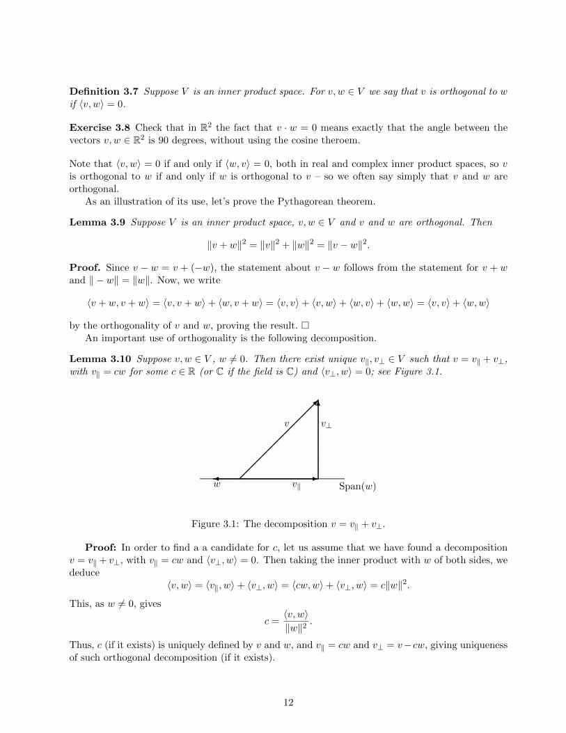
Lemma 3.10 Suppose v, w ∈ V , w 6= 0. Then there exist unique v‖, v⊥ ∈ V such that v = v‖ + v⊥,with v‖ = cw for some c ∈ R (or C if the field is C) and 〈v⊥, w〉 = 0; see Figure 3.1.

. .............................................................................................................................................................................................................................................................................................................................................................................................................................................................................

Span(w).

...............................................................................................................................................................................................................................................................................................................................................

✓

v

.

............................................................................................................................................................................................................................................................

6

v?

. ............................................................................................................................................................................................................................................................ -vk

. ....................................................................................�w

Figure 3.1: The decomposition v = v‖ + v⊥.

Proof: In order to find a a candidate for c, let us assume that we have found a decompositionv = v‖+ v⊥, with v‖ = cw and 〈v⊥, w〉 = 0. Then taking the inner product with w of both sides, wededuce

〈v, w〉 = 〈v‖, w〉+ 〈v⊥, w〉 = 〈cw,w〉+ 〈v⊥, w〉 = c‖w‖2.

This, as w 6= 0, gives

c =〈v, w〉‖w‖2

.

Thus, c (if it exists) is uniquely defined by v and w, and v‖ = cw and v⊥ = v−cw, giving uniquenessof such orthogonal decomposition (if it exists).

12

To show that the orthogonal decomposition does exist, we take

c =〈v, w〉‖w‖2

, v‖ = cw, v⊥ = v − cw,

then both v⊥ + v‖ = v and v‖ = cw are satisfied automatically, so we merely need to checkthat 〈v⊥, w〉 = 0. But we have

〈v⊥, w〉 = 〈v, w〉 − c〈w,w〉 = 〈v, w〉 − 〈v, w〉‖w‖2

‖w‖2 = 0,

so the desired vectors v⊥ and v‖ indeed exist. �One calls v‖ the orthogonal projection of v onto the span of w. We will soon see the following

general version of this statement.

Lemma 3.11 Let V be an inner product vector space, and W a subspace of V spanned by a finitecollection of vectors {w1, . . . , wN}. Then for any v ∈ V there exists a unique pair of vectors v‖and v⊥ so that, v = v‖ + v⊥, v‖ ∈ W and the vector v⊥ has the property that 〈w, v⊥〉 = 0 forany w ∈W .

We will not prove this lemma now but later when it will be actually useful.It will be often very useful to be able to estimate the inner product using the norm. This is

achieved by the Cauchy-Schwarz inequality, a generalization of the Cauchy-Schwarz inequality wehave seen for the dot product in Rn.

Lemma 3.12 (Cauchy-Schwarz) In an inner product space V ,

|〈v, w〉| ≤ ‖v‖‖w‖, v, w ∈ V. (3.14)

For real-valued function spaces, the Cauchy-Schwarz inequality says explicitly that∣∣∣ ∫ 1

0f(x)g(x) dx

∣∣∣ ≤ (∫ 1

0f(x)2 dx

)1/2(∫ 1

0g(x)2 dx

)1/2. (3.15)

A direct proof of the functional inequality (3.15), without using the Cauchy-Schwartz inequality, isactually not so trivial!

Exercise 3.13 Verify that the proof of the Cauchy-Schwartz inequality we presented in Rn worksverbatim in any vector space. We present below an alternative, more geometric proof that uses theorthogonal decomposition.

Proof. If w = 0, then both sides of (3.14) vanish, so we may assume w 6= 0. Write v = v‖ + v⊥ asin Lemma 3.10, so that

v‖ = cw, c =〈v, w〉‖w‖2

, 〈v‖, v⊥〉 = 0.

The last condition above allows us to use the Pythagorean theorem (Lemma 3.9), which gives

‖v‖2 = ‖v‖‖2 + ‖v⊥‖2 ≥ ‖v‖‖2 = |c|2‖w‖2 =|〈v, w〉|2

‖w‖4‖w‖2 =

|〈v, w〉|2

‖w‖2.

Multiplying through by ‖w‖2 and taking the non-negative square root completes the proof of thelemma. �

A useful consequence of the Cauchy-Schwarz inequality is the triangle inequality for the norm:

13

Lemma 3.14 In an inner product space V , we have

‖v + w‖ ≤ ‖v‖+ ‖w‖, for all v, w ∈ V .

Exercise 3.15 Verify that the proof of the triangle inequality in Rn applies verbatim.

In general, regardless of the inner product structure, one defines the notion of a norm on a vectorspace V as follows.

Definition 3.16 Suppose V is a vector space. A norm on V is a map ‖.‖ : V → R such that

1. (Positive definiteness) ‖v‖ ≥ 0 for all v ∈ V , and v = 0 if and only if ‖v‖ = 0.

2. (Absolute homogeneity) ‖cv‖ = |c| ‖v‖, v ∈ V , and c a scalar (so c ∈ R or c ∈ C, dependingon whether V is real or complex),

3. (Triangle inequality) ‖v + w‖ ≤ ‖v‖+ ‖w‖ for all v, w ∈ V .

Thus, Lemma 3.14 shows that the map ‖.‖ : V → R we defined on an inner product spaceis indeed a norm in this sense, so our use of the word norm was justified. Note that (2) impliesimmediately that ‖0V ‖ = 0, where 0V in the left is the zero in V , and 0 in the right is the numberzero. Unless otherwise specified, when we talk of a norm on an inner product space V , we alwaysmean ‖v‖ = 〈v, v〉1/2.

Here are some other examples of a norm on Rn, other than the norm coming from the standarddot product. First, for x = (x1, . . . , xn) ∈ Rn, set

‖(x1, . . . , xn)‖1 =n∑

j=1

|xj |.

The triangle inequality for this norm follows from that on R, the other two properties (positivityand absolute homogeneity) are immediate. This norm is known as the `1-norm on Rn.

The second example is the norm, also on Rn:

‖(x1, . . . , xn)‖∞ = max{|xj | : j = 1, . . . , n}.

This norm is known as the `∞-norm on Rn. The triangle inequality comes from the fact that foreach j, we have

|xj + yj | ≤ |xj |+ |yj |,

so this is also true for any j maximizing |xj + yj | (there may be several such j). Using that j, wecan write

‖x+ y‖∞ = |xj + yj | ≤ |xj |+ |yj | ≤ ‖x‖∞ + ‖y‖∞.

As a side remark, more generally, given any p ≥ 1, we can define the following norm on Rn:

‖(x1, . . . , xn)‖p = (|x1|p + |x2|p + · · ·+ |xn|p)1/p. (3.16)

Positive and positive homogeneity are easy to check for this norm, known as the `p-norm on Rn.The triangle inequality is slightly trickier to prove, and we will do it later. The norm coming fromthe standard dot product in Rn is known as the `2-norm.

Note also that if V is an inner product space then the inner product of a pair of vectors can beexpressed in terms of the corresponding norm as

〈x, y〉 =1

4

(‖x+ y‖2 − ‖x− y‖2). (3.17)

14

However, not all norms on vector spaces come from an inner product. One way to see if the normcomes from the inner product or not, is to verify if (3.17) defines an inner product, that is, if theoperation defined by (3.17) satisfies properties (1)-(3) in Definition 3.3. Note that positivity andsymmetry are automatic: if ‖ · ‖ is a norm satisfying Definition 3.16 then properties (1) and (2) inthis definition immediately imply positivity and symmetry of the ”inner product” defined by (3.17)(the quotation marks refer to the fact that we do not know for a given norm if (3.17) defines aninner product or not). However, the linearity in the first slot, property (2) in Definition 3.3 does nothold for all norms. For example, for the `∞ norm, we can take

v = (1, 1), w = (0, 1)

and observe that, with the definition

〈x, y〉∞ =1

4

(‖x+ y‖2∞ − ‖x− y‖2∞), (3.18)

we would have

〈v, w〉∞ =1

4

(‖(1, 2)‖2∞ − ‖(1, 0)‖2∞) =

1

4(4− 1) =

3

4

but note that

−3

4v + w =

(− 3

4,1

4

), − 3

4v − w =

(− 3

4,−7

4

)hence

〈(− 3

4

)v, w〉∞ =

1

4

(‖(−3

4,1

4)‖2∞ − ‖(−

3

4,−7

4)‖2∞) =

1

4

( 9

16− 49

16

)= −5

86= −3

4· 3

4= −3

4〈v, w〉∞.

Thus, the `∞-norm does not come from an inner product on Rn.

Exercise 3.17 Show that the `1-norm also does not come from an inner product on Rn.

4 Gaussian elimination and the linear dependence lemma

Our goal in this section is to prove the following lemma.

Lemma 4.1 (The linear dependence lemma) Let v1, . . . , vk be a collection of k vectors in a vectorspace V . Then any collection w1, w2, . . . wk+1 of k + 1 vectors in the span of v1, . . . , vk is linearlydependent.

We will assume that V is a vector space over R but the proof is verbatim the same for a vector spaceover any field F. It may be helpful for the reader to focus on the situation when V = Rn as thisdoes not change anything in the arguments or statements in this section.

In order to show that the vectors w1, w2, . . . , wk+1 are linearly dependent, we need to find realnumbers x1, x2, . . . , xk+1 such that not all of xj equal to zero, and

x1w1 + x2w2 + · · ·+ xk+1wk+1 = 0. (4.1)

Note that this is a vector identity: the left side is a vector in V , and the 0 in the right side is the zerovector in V . Let us translate (4.1) into a system of linear equations for the unknowns x1, . . . , xk+1.Since each vector wj is in the span of v1, . . . , vk, it is a linear combination of the vectors v1, . . . , vk.Thus, there exist real numbers ajm, j = 1, . . . , k, m = 1, . . . , k + 1, so that

wm = a1mv1 + a2mv2 + · · ·+ akmvk. (4.2)

15

Substituting these expressions into (4.1) gives

x1(a11v1 + a21v2 + · · ·+ ak1vk) + x2(a12v1 + a22v2 + · · ·+ ak2vk) + . . .

+ xk+1(a1,k+1v1 + a2,k+1,2v2 + · · ·+ ak,k+1vk) = 0,(4.3)

which can be re-written as

(a11x1 + a12x2 + · · ·+ a1,k+1xk+1)v1 + (a21x1 + a22x2 + · · ·+ a2,k+1xk+1)v2 + . . .

+ (ak1x1 + ak2x2 + · · ·+ ak,k+1xk+1)vk = 0.(4.4)

Equality (4.4) holds, clearly, if we find real numbers x1, . . . , xk+1 such that

a11x1 + a12x2 + · · ·+ a1,k+1xk+1 = 0

a22x1 + a22x2 + · · ·+ a2,k+1xk+1 = 0

... . . ....

ak1x1 + ak2x2 + · · ·+ ak,k+1xk+1 = 0.

(4.5)

Note that while (4.4) is an equality in V – the left side is a vector in V and the right side is thezero vector in V , the system (4.5) involves only real numbers. This is a homogeneous system of kequations for (k + 1) unknowns x1, . . . , xk+1 – recall that the coefficients amj are given. Our taskis to show that it always has a solution, such that not all of xj equal to zero, no matter whatthe numbers amj are. More generally, we will consider systems of m equations for n unknown realnumbers x1, . . . , xn:

a11x1 + a12x2 + · · ·+ a1nxn = 0

a21x1 + a22x2 + · · ·+ a2nxn = 0

... . . ....

am1x1 + am2x2 + · · ·+ amnxn = 0,

(4.6)

with m < n and show that it always has a non-zero solution. Such systems are known as homoge-neous because the right side is zero. This means that if (x1, . . . , xn) is a solution of (4.6) then forany λ ∈ R, the numbers x′1 = λx1, x

′2 = λx2, . . . , x

′n = λxn also provide a solution, hence the name

”homogeneous”.

Lemma 4.2 A homogeneous system (4.6) of m linear equations for n unknown real numbers x1, . . . , xn,with m < n, always has a solution such that not all of xj equal to zero.

As we have explained, Lemma 4.1 follows from Lemma 4.2, so our goal is to prove the latter.

4.1 Gaussian elimination

We will prove Lemma 4.2 using what is known as the Gaussian elimination procedure. The firstobservation is that the set of solutions of the system (4.6) does not change under the followingoperations:(1) Interchange any pair of equations.(2) Multiply one of the equations by a non-zero constant.(3) Add a multiple of one equation to another. For example, take equation j and add it to equation iwith i 6= j.

16

Gaussian elimination is the following process of finding a solution to (4.6). If all coefficients inthe first column vanish: aj1 = 0 for all 1 ≤ j ≤ m, so that the system has the form

0x1 + a12x2 + · · ·+ a1nxn = 0

0x1 + a22x2 + · · ·+ a2nxn = 0

... . . ....

0x1 + am2x2 + · · ·+ amnxn = 0,

(4.7)

then a solution to (4.7) is simply x1 = 1 and x2 = · · · = xn = 0 – hence, we found a solution. If notall aj1 = 0, then by interchanging the rows we may assume without loss of generality that a11 6= 0.We divide the first equation by a11 – this does not affect all other equations, and re-write (4.6) as

x1 + a12x2 + · · ·+ a1nxn = 0

a21x1 + a22x2 + · · ·+ a2nxn = 0

... . . ....

am1x1 + am2x2 + · · ·+ amnxn = 0,

(4.8)

where a1j = a1j/a11. Next, we subtract from each equation j ≥ 2 the first equation multipliedby aj1. Then the system will have the form

x1 + a12x2 + · · ·+ a1nxn = 0

0x1 + a22x2 + · · ·+ a2nxn = 0

... . . ....

0x1 + am2x2 + · · ·+ amnxn = 0,

(4.9)

with the coefficients in the first row unchanged from the previous step: a1j = a1j , and the coefficientsin the other rows changed, so that, for instance, a22 = a22 − a21a12, and generally,

ajk = ajk − aj1a1k.

Again, if all aj2 = 0, we can take x2 = 1 and all other xj = 0, otherwise, we can find j ≥ 2 sothat aj2 6= 0, and move that equation into the second row. In other words, we may assume withoutloss of generality that a22 6= 0. We divide now the second row by a22:

x1 + a12x2 + · · ·+ a1nxn = 0

0x1 + x2 + · · ·+ a2nxn = 0

... . . ....

0x1 + am2x2 + · · ·+ amnxn = 0.

(4.10)

We can now eliminate x2 from all but the first two equations, in the same way as we eliminated x1from all but the first equation, and then continue this process with x3, and so on, known as theGaussian elimination.

4.2 The proof of Lemma 4.2

The proof of Lemma 4.2 is by induction, and does not use the full Gaussian elimination. Instead,we observe that when m = 1, the system (4.6) consists of just one equation:

a11x1 + a12x2 + · · ·+ a1nxn = 0, (4.11)

17

for n > 1 unknowns. If all a1j = 0 then we simply set x1 = 1 and all other xj = 0. Otherwise, if,say, a11 6= 0, then we take any x2, . . . , xn and set

x1 = −a12a11

x2 − · · · −a1na11

xn.

Thus, the conclusion of the lemma holds for m = 1 and all n > 1. Next, assume that it holds forsome m and all n > m. Then, given a system of m+1 equations with n > m+1 unknowns, we applythe Gaussian elimination to obtain a system of m equations for n− 1 > m unknowns x2, . . . , xn. Ithas a solution by the induction assumption, and x1 can then be found from the first equation in thesystem obtained after one step of the Gaussian elimination, and we are done. �

As we have discussed, Lemma 4.1 is a consequence of Lemma 4.2, thus Lemma 4.1 is proved aswell.

5 The basis theorem

We now turn to the notion of a basis of a vector space. Let us first give a general definition of abasis of a vector space.

Definition 5.1 A collection of vectors {v1, v2, . . . , vN} is a basis for a vector space V if {v1, v2, . . . , vN}are linearly independent and V = span{v1, v2, . . . , vN}.

A canonical example of a basis is the collection of vectors

e1 = (1, 0, . . . , 0), e2 = (0, 1, 0, . . . , 0), . . . , en = (0, 0, . . . , 0, 1) (5.1)

in Rn. Note that for real numbers x1, x2, . . . , xn ∈ R, we have

x1e1 + x2e2 + · · ·+ xnen = (x1, x2, . . . , xn). (5.2)

This identity implies that ek, k = 1, . . . , n are linearly independent, for if we have

x1e1 + · · ·+ xnen = 0,

for some real numbers x1, x2, . . . , xn ∈ R, then (5.2) shows that all xk = 0. Moreover, e1, . . . , en,form a basis of Rn because any vector (c1, . . . , cn) ∈ Rn can be written as

c = c1e1 + c2e2 + · · ·+ cnen,

hence Rn is spanned by e1, . . . , en. In particular, Rn is the span of the vectors e1, . . . , en and thusno collection of more than n vectors in Rn can be linearly independent, according to Lemma 4.1.

Exercise 5.2 Another example of a basis in a vector space is the following. Let Pm be the vectorspace of all polynomials of degree less or equal to m. Show that the polynomials

p0(x) = 1, p1(x) = x, . . . , pm(x) = xm

form a basis of Pm.

18

5.1 The basis theorem in Rn

The first main result of this section is the following.

Theorem 5.3 Any non-trivial subspace of Rn has a basis.

Proof. Let V be a subspace of Rn and let q be the largest integer such that there exist q linearlyindependent vectors v1, . . . , vq in V . Note that q ≤ n – as we have noted above, Lemma 4.1 impliesthat no collection of more than n vectors can be linearly independent in Rn. We claim that V isthe span of {v1, . . . , vq}. Indeed, as all vj belong to V , we know that span{v1, . . . , vq} is a sub-spaceof V . Let us assume that there is a vector w ∈ V such that w is not in span{v1, . . . , vq}. It followsfrom the way q was chosen, that the collection {v1, . . . , vq, w} is linearly dependent. Hence, thereexist real numbers a1, . . . , aq and b, such that they are not all equal to zero, and

a1v1 + · · ·+ aqvq + bw = 0.

If b = 0 then not all of aj are zero, and

a1v1 + · · ·+ aqvq = 0,

which is a contradiction to the linear independence of {v1, . . . , vq}. Hence, b 6= 0, but then we canwrite

w = −a1bv1 − · · · −

aqbvq,

showing that w is in span{v1, . . . , vq}, which is a contradiction. Thus, we have V = span{v1, . . . , vq},and, as these vectors are linearly independent, they form a basis for V . �

The next result shows that any linearly independent set of vectors in a sub-space can be completedto form a basis of the sub-space.

Theorem 5.4 Let V be a subspace of Rn and u1, . . . , uk be a collection of linearly independentvectors in V . Then it can be extended to form a basis, that is, there exists a basis v1, . . . , vq of Vwith q ≥ k such that v1 = u1, v2 = u2, . . . , vk = uk.

Proof. Similarly to the proof of Theorem 5.3, let q be the largest integer so that there exists acollection of q linearly independent vectors in V such that v1 = u1, v2 = u2, . . . , vk = uk. Arguingexactly as in the previous proof, we can show that V is the span of {v1, . . . , vq}. As these vectorsare linearly independent they form a basis for V , which, by construction, satisfies the requirementof the present theorem. �

Theorem 5.5 Let V be a sub-space of Rn. Then every basis of V has the same number of vectors.

Proof. Assume that V has two bases, {v1, . . . , vq} and {w1, . . . , wk} with q > k. As {w1, . . . , wk} isa basis for V , we know that V = span{w1, . . . , wk}. As q > k, Lemma 4.1 implies that the vectors{v1, . . . , vq} are linearly dependent, which is a contradiction. �

5.2 Finite-dimensional vector spaces

Definition 5.6 A vector space V is called finite dimensional if there is a finite subset {v1, . . . , vn}of elements of V such that Span{v1, . . . , vn} = V . We say that V is n-dimensional if it has a basisthat contains exactly n vectors.

19

The most standard example of an n-dimensional vector space is Rn. An example of a k-dimensionalvector space is Wk = {x ∈ Rn : x1 = x2 = · · · = xn−k = 0}. Another example of an n-dimensionalvector space is Vn = {x ∈ Rn+1 : x1 + x2 = 0}.

Not every vector space is finite-dimensional.

Exercise 5.7 Show that the vector space P of all polynomials is not finite-dimensional.

Exactly as in Rn, we have the following versions of Theorems 5.3 and 5.4, with essentially identicalproofs to those of these two theorems.

Theorem 5.8 Any non-trivial subspace of a finite-dimensional vector space V has a basis.

Theorem 5.9 Let V be a subspace of a finite-dimensional space W and u1, . . . , uk be a collectionof linearly independent vectors in V . Then there exists a basis v1, . . . , vq of V with q ≥ k such thatv1 = u1, v2 = u2, . . . , vk = uk.

Exercise 5.10 Explain how the proofs of Theorems 5.3 and 5.4 rely on the fact that Rn is a finite-dimensional vector space.

Theorem 5.11 Let V be an n-dimensional vector space. Then (i) any collection of n linearlyindependent vectors {v1, . . . , vn} is a basis for V , and (ii) any collection of n vectors that span Vmust be linearly independent.

Proof. For (i), note that since V is n-dimensional, it is a span of n basis vectors. Lemma 4.1implies that given any w ∈ V , the collection {v1, . . . , vn, w} is linearly dependent. As {v1, . . . , vn}are linearly independent, as in the proof of Theorem 5.3, it follows that w can be written as

w = a1v1 + · · ·+ anvn.

As this is true for any vector w ∈ V , we conclude that {v1, . . . , vn} span V , and, as they are linearlyindependent, they form a basis for V . As for part (ii), assume that {v1, . . . , vn} span V but arelinearly dependent. It follows then from Lemma 2.10 that there exists some j 6= n and real numbersc1, . . . , cj−1, cj+1, . . . , cn, such that

vj = c1v1 + · · ·+ cj−1vk−1 + ck+1vk+1 + · · ·+ cnvn. (5.3)

It follows that V is the span of (n − 1) vectors {v1, . . . , vj−1, vj+1, . . . , vn} and thus V can not ben-dimensional by Lemma 4.1. �

Given a basis {v1, . . . , vn} of an n-dimensional vectors space V and a vector z ∈ V there is aunique way to represent z as a linear combination

z = z1v1 + · · ·+ znvn, (5.4)

with some z1, . . . , zn ∈ R. The numbers z1, . . . , zn are called the coordinates of z in the basis{v1, . . . , vn}.

Exercise 5.12 Show that the map T (z) = (z1, . . . , zn) defined above is a one-to-one and onto mapfrom V to Rn, such that for all λ, µ ∈ R and z, y ∈ V we have T (λz + µy) = λT (z) + µT (y).

6 Matrices and maps

So far, linear algebra was all about vector spaces. Now we turn to its true subject: linear mapsbetween vector spaces.

20

6.1 Matrices of linear transformations in the standard basis in Rn

In this section, we we will look at the matrix representations for linear maps T : Rn → Rm.

Definition 6.1 We say that T : Rn → Rm is a linear map from Rn to Rm if for every v ∈ Rn, thevector w = T (v) is in Rm, and the map T has the property that for any x, y ∈ Rn and λ, µ ∈ R wehave

T (λx+ µy) = λT (x) + µT (y). (6.1)

Note that (6.1) is an identity in Rm: both sides are vectors in Rm.An example of a linear map R2 → R2 is the rotation in R2 by an angle α:

T (x1, x2) = (x1 cosα− x2 sinα, x1 sinα+ x2 cosα).

Note that if x = (r cosφ, r sinφ), then

T (x) = (r cosφ cosα− r sinφ sinα, r cosφ sinα+ r sinφ cosα) = (r cos(α+ φ), r sin(α+ φ)),

so that this, indeed, a rotation by an angle α. Another standard example is a dilation in Rn by areal number λ: T (x1, . . . , xn) = (λx1, . . . , λxn). More generally, we may fix real numbers λ1, . . . , λnand define a map T : Rn → Rn as

T (x1, . . . , xn) = (λ1x1, . . . , λnxn).

A typical example of a map T : Rn → Rm with m < n is a projection:

T (x1, . . . , xm, xm+1, . . . , xn) = (x1, . . . , xm).

A typical example of a map T : Rn → Rm with m > n is

T (x1, . . . , xn) = (x1, . . . , xn, 0, . . . , 0).

A way to represent the action of a linear T on Rn is in terms of matrices. This is done asfollows. Let e1, . . . , en be the standard basis for Rn and e1, . . . , em be the standard basis for Rm.The vectors T (ej), j = 1, . . . , n lie in Rm, thus they can be represented as linear combinations of ek:there exist numbers ajk, j = 1, . . . ,m, k = 1, . . . , n, so that

T (ek) = a1ke1 + · · ·+ amkem. (6.2)

Let x = (x1, . . . , xn) ∈ Rn be a vector in Rn. The linearity of T implies that we can write

T (x) = T (x1e1 + · · ·+ xnen) = x1T (e1) + · · ·+ xnT (en). (6.3)

This can be expanded using (6.2)

T (x) = x1T (e1) + · · ·+ xnT (en) = x1[a11e1 + a21e2 + · · ·+ am1em]

+ x2[a12e1 + a22e2 + · · ·+ am2em] + · · ·+ xn[a1ne1 + a2ne2 + · · ·+ amnem].(6.4)

Collecting the terms in front of each ek gives

T (x) = [a11x1 + a12x2 + · · ·+ a1nxn]e1 + [a21x1 + a22x2 + · · ·+ a2nxn]e2 + . . .

+ [am1x1 + am2x2 + · · ·+ amnxn]em.(6.5)

21

That is, if know the numbers aij that are determined solely by the action of the transformation Ton the vectors ek that form the standard basis, then the action of T on any vector x can be writtenas

T (x1, . . . , xn) = (a11x1+a12x2+· · ·+a1nxn, a21x1+a22x2+· · ·+a2nxn, . . . , am1x1+am2x2+· · ·+amnxm).(6.6)

This motivates the following definition. Let A be an m × n matrix (m rows and n columns), andx ∈ Rn, then the product Ax is a vector in Rm that is given by the right side of (6.6). It is convenientto reprsent this multiplication in terms of vector columns:

y = Ax

is denoted as y1y2...ym

=

a11 a12 . . . a1na21 a22 . . . a2n...

......

...

am1 am2 . . . amn

x1x2...xn

. (6.7)

Note that (a1k, a2k, . . . , amk), the k-th column of the matrix A is simply the vector T (ek) – the imageof the vector ek under tha map T .

One can add linear transformations T1 and T2 that both map Rn to Rm:

(T1 + T2)(x) = T1(x) + T2(x). (6.8)

It is easy to see that if the matrices corresponding to T1 and T2 are, respectively, T1 and T2, thenthe mapping T1 + T2 corresponds to the matrix A+B, with the entries

(A+B)ij = aij + bij . (6.9)

Note that one can only add matrices of the same size.

6.2 Matrices of linear transformations for finite-dimensional vector spaces

An essentially identical procedure of representing a linear transformation in terms of a matrix worksfor general linear maps between two finite-dimensional vector spaces V and W . We will assumethat V and W are vector spaces over R but the construction is identical for vector spaces over anarbitrary field F.

Definition 6.2 We say that T : V →W is a linear map from V to W if for every v ∈ V , the vectorw = T (v) is in W , and the map T has the property that for any x, y ∈ V and λ, µ ∈ R we have

T (λx+ µy) = λT (x) + µT (y). (6.10)

Again, (6.10) is an identity in the vector space W .As for maps from Rn to Rm, we can represent maps from V to W by matrices after we fix a basis

in V and a basis in W , except now we will relate the coordinates of a vector v ∈ V , in some fixedbasis in V to the coordinates of the vector T (v) ∈W expressed in some fixed basis in W . The ideais exactly as before. Let {v1, . . . , vn} be a basis for V , with n = dimV , and {w1, . . . , wm} be ta basisfor W , with m = dimW . The vectors T (vj), j = 1, . . . , n lie in W , thus they can be represented aslinear combinations of wk: there exist numbers ajk, j = 1, . . . ,m, k = 1, . . . , n, so that

T (vk) = a1kw1 + · · ·+ amkwm. (6.11)

22

Now, let x ∈ V be a vector in V , with the coordinates (x1, . . . , xn) in the basis {v1, . . . , vn}:

x = x1v1 + · · ·+ xnvn.

The linearity of T implies that we can write

T (v) = T (x1v1 + · · ·+ xnvn) = x1T (v1) + · · ·+ xnT (vn). (6.12)

This can be expanded using (6.11)

T (x) = x1T (v1) + · · ·+ xnT (vn) = x1[a11w1 + a21w2 + · · ·+ am1wm]

+ x2[a12w1 + a22w2 + · · ·+ am2wm] + · · ·+ xn[a1nw1 + a2nw2 + · · ·+ amnwm].(6.13)

Collecting the terms in front of each wk gives

T (x) = [a11x1 + a12x2 + · · ·+ a1nxn]w1 + [a21x1 + a22x2 + · · ·+ a2nxn]w2 + . . .

+ [am1x1 + am2x2 + · · ·+ amnxm]wm.(6.14)

That is, if know the numbers aij that are determined solely by the action of the transformation T onthe vectors vk that form the basis we are using in V , then if a vector x has coordinates (x1, . . . , xn)in the basis {v1, . . . , vn} in V , then the coordinates of the vector T (x) in the basis {w1, . . . , wn}in W are

T (x) = y1w1 + · · ·+ ynwn,

with the vector y ∈ Rm (note that the coordinates of T (x) can be written as an m-tuple of realnumbers, hence an element of Rm)

(y1, . . . , ym) = (a11x1+a12x2+· · ·+a1nxn, a21x1+a22x2+· · ·+a2nxn, . . . , am1x1+am2x2+· · ·+amnxn).(6.15)

As in (6.7), this relation can be written as

y1y2...ym

=

a11 a12 . . . a1na21 a22 . . . a2n...

......

...

am1 am2 . . . amn

x1x2...xn

, (6.16)

or, in the matrix-mltiplied-by-a-vector vector form, as

y = Ax.

6.3 Composition of maps

An important operation between maps is a composition. Given vectors spaces V1, V2 and V3 andlinear maps T1 : V1 → V2 that maps V1 to V2 and T2 : V2 → V3 that maps V2 to V3, we may definetheir composition T2 ◦ T1 : V1 → V3 as (T2 ◦ T1)(v) = T2(T1(v)), for v ∈ V1.

Lemma 6.3 Suppose V , W and Z are vector spaces, and T : V → W and S : W → Z are linearmaps, then S ◦ T : V → Z is a linear map as well.

23

Proof. For any λ, µ ∈ R and x, y ∈ V we have

(S ◦T )(λx+µy) = S(T (λx+µy)) = S(λTx+µTy) = λS(Tx)+µS(Ty) = λ(S ◦T )(x)+µ(S ◦T )(y),

which shows that the map S ◦ T is linear. �Next, we compute the matrix of a composition of two linear maps. Let us assume that the

spaces V1, V2 and V3 are finite-dimensional, and denote nk = dimVk, with k = 1, 2, 3. We fix a basis

{v(1)1 , . . . , v(1)n1 } in V1, a basis {v(2)1 , . . . , v

(2)n2 } in V2, and, finally, a basis {v(3)1 , . . . , v

(3)n3 } in V3. Let A

be the matrix of the map T1 with respect to the bases {v(1)1 , . . . , v(1)n1 } in V1 and {v(2)1 , . . . , v

(2)n2 } in V2,

and B be the matrix of the map T2 with respect to the bases {v(1)2 , . . . , v(2)n2 } in V2 and {v(3)1 , . . . , v

(3)n3 }

in V3. Our goal is to compute the matrix of the map T2 ◦ T1 : V1 → V3, with respect to the bases

{v(1)1 , . . . , v1)n1} in V1 and {v(3)1 , . . . , v

3)n3} in V3. We first write

(T2 ◦ T1)(v(1)k ) = T2(T1(v(1)k )), k = 1, . . . , n1. (6.17)

As in (6.11), we can write, using the summation notation

T1(v(1)k ) = a1kv

(2)1 + · · ·+ an2kv

(2)n2

=

n2∑j=1

ajkv(2)j , (6.18)

for each k = 1, . . . , n1. Applying T2 to both sides of this identity gives, using the linearity of T2:

(T2 ◦ T1)(v(1)k ) = T2(T1(v(1)k )) = T2

( n2∑j=1

ajkv(2)j

)=

n2∑j=1

ajkT2(v(2)j ). (6.19)

Recall that B is the matrix of the map T2 with respect to the bases {v(1)2 , . . . , v2)n2} in V2 and

{v(3)1 , . . . , v(3)n3 } in V3, so that

T2(v(2)j ) = b1jv

(3)1 + · · ·+ bn3jv

(3)n3

=

n3∑m=1

bmjv(3)m . (6.20)

Using this expression in the right side of (6.19) gives

(T2 ◦ T1)(v(1)k ) =

n2∑j=1

ajkT2(v(2)j ) =

n2∑j=1

ajk

n3∑m=1

bmjv(3)m =

n2∑j=1

n3∑m=1

ajkbmjv(3)m . (6.21)

Interchanging the order of summation in m and j we can write this as

(T2 ◦ T1)(v(1)k ) =

n3∑m=1

n2∑j=1

bmjajkv(3)m =

n3∑m=1

( n2∑j=1

bmjajk

)v(3)m . (6.22)

Setting

cmk =

n2∑j=1

bmjajk, (6.23)

we obtain

(T2 ◦ T1)(v(1)k ) =

n3∑m=1

cmkv(3)m . (6.24)

Therefore, the matrix C of the composition map T2 ◦ T1, with respect to the bases {v(1)1 , . . . , v1)n1} in

the space V1 and {v(3)1 , . . . , v3)n3} in the space V3 has the entries given by (6.23). This motivates the

following definition.

Definition 6.4 Let A be an m2×m1 matrix and B be an m3×m2 matrix, then the product C = BAis the m3 ×m1 matrix, with the entries given by (6.23).

24

7 Rank of a map and a matrix and the rank-nullity theorem

Once again, we use in this section vector spaces over R but the results hold verbatim for vectorspaces over nay other field F.

7.1 The kernel and the range of a map and of a matrix

Two extremely important notions associated to a linear map T are the null space and the range.

Definition 7.1 (i) The nullspace, or kernel of a linear map T : V →W is the set {x ∈ V : Tx = 0},denoted as N(T ) or KerT(ii) The range, or image of a linear map T : V → W is the set {Tx : x ∈ V }, denoted as RanTor ImT

Exercise 7.2 Let T : V → W be a linear map from a vector space V to a vector space W . Showthat KerT is a sub-space in V and RanT is a subspace of W .

The notions of the kernel and the range can be extended from maps to matrices. Consider a basis{v1, . . . , vn} in V , with n = dimV and a basis {w1, . . . , wm} in W , with m = dimW . Let A be thematrix of T in these bases, and z ∈ V be a vector in N(T ): T (z) = 0. If we write z in terms of itscoordinates in the basis {v1, . . . , vn}:

z = z1v1 + · · ·+ znvn,

then the fact that T (z) = 0 is equivalent to the ”matrix-times-a-vector” identity

Az = 0,

where z = (z1, . . . , zn) ∈ Rn is the n-tuple of coordinates of the vector z ∈ V . Because of that, wesay that a vector x ∈ Rn is in the kernel of an m×n matrix A if Ax = 0. We say that a vector y ∈ Rn

is in the range of A if there exists x ∈ Rn so that Ax = y. In other words, we have

KerA = {x ∈ Rn : Ax = 0}, RanA = {y ∈ Rm such that there exists x ∈ Rn so that Ax = y.(7.1)

A digression: the inverse map. Recall that a map f : X → Y between sets X,Y has aninverse if and only if it is one-to-one. In other words, f(x) is defined uniquely for each x ∈ Xand for each y ∈ Y there exists exactly one element x ∈ X such that f(x) = y. In that case, onedefines f−1(y) as the unique element x of X such that f(x) = y. If T : V → W is linear andbijective, so it has an theoretic inverse, this inverse is necessarily linear.

Lemma 7.3 If T : V →W is linear and one-to-one, then the inverse map T−1 is linear.

Proof. Indeed, let T−1 be this map. Then

T (T−1(λx+ µy)) = λx+ µy

by the definition of T−1, and

T (λT−1x+ µT−1y) = λTT−1x+ µTT−1y = λx+ µy

where the first equality is the linearity of T and the second the definition of T−1. Thus,

T (T−1(λx+ µy)) = T (λT−1x+ µT−1y),

25

so since T is one-to-one,T−1(λx+ µy) = λT−1x+ µT−1y,

proving linearity. �Here is the relation between a linear map being one-to-one and its null space.

Lemma 7.4 A linear map T : V → W is a one-to-one map from V to RanV ⊆ W if and onlyif N(T ) = {0}.

Proof: Since T (0) = 0 (the 0 in the left side being in V and in the right side in W ) for any linearmap, if T is one-to-one, the only element of V it may map to 0 ∈W is 0 ∈ V , so N(T ) = {0}.

Conversely, suppose that N(T ) = 0. If Tx = Tx′ for some x, x′ ∈ V then

Tx− Tx′ = 0

henceT (x− x′) = 0.

Since N(T ) = {0}, it follows that x− x′ = 0, and x = x′, showing for every y ∈ RanT there existsexactly one x ∈ V such that T (x) = y. �

Lemma 7.5 If T : V →W is a linear map, and v1, . . . , vn span V , then RanT = Span{Tv1, . . . .T vn}.

Note that this lemma shows that if V is finite dimensional, then RanT is finite dimensional, evenif W is not. Another immediate consequence is that if dim(RanT ) ≤ dimV . The rank-nullitytheorem below will address what has to happen to gave dim(RanT ) < dimV .Proof of Lemma. We have

RanT = {Tx : x ∈ V } ={T (

n∑j=1

cjvj) : c1, . . . , cn ∈ R}

={ n∑

j=1

cjTvj : c1, . . . , cn ∈ F}

= Span{Tv1, . . . .T vn}.

Here, the first equality is the definition of the range, the second uses the fact that v1, . . . , vn span V ,the third uses the linearity of T , and the last one uses the definition of the space of Tv1, . . . , T vn. �

7.2 The column and the row spaces of a matrix

As we have noted below (6.7), if T : Rn → Rm, written as a matrix A in the standard bases, thenthe kth column of the matrix A is Tek, where ek ∈ Rn is the kth standard basis vector in Rn. Thus,the column space C(A) of the matrix A of a map T : Rn → Rm, written in the standard bases,which is by definition the span of the vectors Tej , j = 1, . . . , n, is RanT by Lemma 7.5.

The row space R(A) of the matrix A is the span of the rows of the matrix, that is, if the matrix Ahas the form

a11 a12 . . . a1na21 a22 . . . a2n...

......

...

am1 am2 . . . amn

,

26

then R(A) the span of m vectors

r1 = (a11, a12, . . . , a1n), r2 = (a21, a22, . . . , a2n), . . . , rm = (am1, am2, . . . , amn).

Note that R(A) is a subspace of Rn. For each x ∈ Rn the vector Ax can be written as

Ax =

a11 a12 . . . a1na21 a22 . . . a2n...

......

...

am1 am2 . . . amn

x1x2...xn

=

r1 · x...

rm · x

. (7.2)

Thus, if x ∈ Rn is in the null space of A then for each k = 1, . . . , n, we have rk · x = 0, hence xis orthogonal to all v ∈ R(A). Conversely, if x ∈ Rn is orthogonal to each v ∈ R(A), then it isorthogonal to each rk, k = 1, . . . ,m, so that rk · x = 0, and thus x ∈ KerA. In other words, Ker(A)is the collection of all vectors x ∈ Rn such that for each v ∈ R(A) we have x · v = 0.

Exercise 7.6 Show that if v ∈ Rn has the property that for all x ∈ Ker(A) we have x · v = 0then v ∈ R(A). Hint: see Section 3 notes on the orthogonal complements.

The terminology is that R(A) is the orthogonal complement of KerA and we write R(A) = (KerA)⊥.

Lemma 7.7 Let v1, . . . , vk be a linearly independent collection of vectors in KerA and vk+1, vj alinearly independent collection of vectors in R(A). Then the collection v1, . . . , vk, vk+1, . . . , vj is alsolinearly independent.

Proof. Note that for each 1 ≤ i ≤ k and k + 1 ≤ j ≤ q we have vi · vj = 0. Assume now that

c1v1 + · · ·+ ckvk + ck+1vk+1 + · · ·+ cjvj = 0

and take the dot product of both sides with x = c1v1 + · · ·+ ckvk. Using the above observation gives

‖c1v1 + c2v2 + · · ·+ ckvk‖2 = 0, (7.3)

so thatc1v1 + c2v2 + · · ·+ ckvk = 0.

As {v1, . . . , vk} are linearly independent we conclude that c1 = c2 = · · · = ck = 0. Using this in (7.3)gives

ck+1vk+1 + · · ·+ cjvj = 0.

Now, the linear independence of vk+1, . . . , vj implies that we also have ck+1 = · · · = cj = 0. �

Lemma 7.8 Every vector x ∈ Rn can be decomposed uniquely as x = v + w with v ∈ KerA andw ∈ R(A).

Proof. Uniqueness is not difficult: if

v1 + w1 = v2 + w2,

with v1, v2 ∈ KerA and w1, w2 ∈ R(A), then

v1 − v2 = w2 − w1.

27

Taking the dot product of both sides with v1−v2 and using the fact that wk ⊥ vj , j, k = 1, 2, we get

‖v1 − v2‖2 = 0,

thus v1 = v2, and then it follows that w1 = w2.Existence is a little trickier. The idea is very similar to what we did in the orthogonal projection

in Lemma 3.10. Fix x ∈ Rn and consider the function φ(v) = ‖x − v‖2, defined for v ∈ KerA.Let v ∈ KerA be a vector in KerA that minimizes the function φ(v). We claim that then (x−v)·z = 0for all z ∈ KerA, which implies that x− v ∈ R(A) by Exercise 7.6. Let us take z ∈ KerA and notethat, since v minimizes φ(v), we have, for all t ∈ R:

‖x− v‖2 ≤ ‖x− v + tz‖2 = ‖x− v‖2 + 2t(x− v) · z + t2‖z‖2.

In other words, the right side is a quadratic function that is minimized at t = 0. It follows that thecoefficient in front of t has to vanish, hence (x − v) · z = 0. Thus, w = x − v ∈ R(A), and we haveconstructed the decomposition. �

Corollary 7.9 We have dim(KerA) + dim(R(A)) = n.

Exercise 7.10 Prove this corollary.

7.3 The rank-nullity theorem

Definition 7.11 Let V and W be finite-dimensional vector spaces and T : V → W a linear map.Then the rank of T , denoted as rank(T ) is the dimension of RanT .

In the same vein, the rank of a matrix A is the dimension of its column space. Note that if A is thematrix of a linear map T in some basis, then the rank of the matrix A equal the rank of the map T .

Let us first make the following observation, continuing the line of thought started in Lemma 7.5.

Proposition 7.12 We have dimV = dim RanT if and only if KerT = {0}.

Proof. Let n = dimV and {v1, . . . , vn} be a basis for V . Note that RanV = span(T (v1), . . . , T (vn)),hence dim RanV ≤ n. First, assume that dim RanT = n, then the vectors T (v1), . . . , T (vn) form acollection that spans RanT and has n = dim(RanT ) vectors, hence {T (v1), . . . , T (vn)} form a basisfor RanT and these vectors are linearly independent. In that case, if v ∈ KerT , we write it as

v = c1v1 + . . . cnvn,

apply T to both sides and conclude that, as v ∈ KerT , we have

0 = T (v) = c1T (v1) + · · ·+ cnT (vn).

The linear independence of T (v1), . . . , T (vn) implies that all ck = 0, hence v = 0, thus, indeed,KerT = {0}. On the other hand, if KerT = {0}, and there exist some ck ∈ R so that

c1T (v1) + · · ·+ cnT (vn) = 0,

then, settingv = c1v1 + . . . cnvn,

we see that T (v) = 0. As KerT = {0}, we conclude that v = 0 and, as v1, . . . , vn are linearly inde-pendent, it follows that all ck = 0. Therefore, the vectors T (v1), . . . , T (vn) are linearly independent,which means that they form a basis of their span, which is RanT , and thus dim(RanT ) = n. �

Proposition 7.12 shows a connection between the dimension of KerT and the dimension of RanT .Here is the general result.

28

Theorem 7.13 (Rank-nullity) Suppose T : V →W is linear with V finite dimensional. Then

dim RanT + dim KerT = dimV.

Proof. We have already considered the case KerT = {0} in Proposition 7.12, so let us assumethat KerT 6= {0}. Let k = dim(KerT ) and let the vectors u1, . . . , uk form a basis for KerT .Theorem 5.9 allows us to complete this set to a basis {u1, . . . , uk, vk+1, . . . , vn} of V . We will showthat the vectors {T (vk+1), . . . , T (vn)} are linearly independent and span RanT , which would implythat dim(RanT ) = n− k, and imply the conclusion of Theorem 7.13. First, note that if

c1T (vk+1) + · · ·+ cnT (vn) = 0,

then the vector c1vk+1+· · ·+cnvn ∈ KerT = span(u1, . . . , uk). As the vectors {u1, . . . , uk, vk+1, . . . , vn}form a basis of V , they are linearly independent, and it follows that all cj = 0, proving the linearindependence of {vk+1, . . . , vn}. Next, if y ∈ RanT , so that y = T (x) with some x ∈ V , we canrepresent x as

x = α1u1 + α2u2 + · · ·+ αkuk + αk+1vk+1 + · · ·+ αnvn.

Applying T to both sides gives

y = T (x) = T (α1u1 + α2u2 + · · ·+ αkuk + αk+1vk+1 + · · ·+ αnvn)

= T (α1u1 + α2u2 + · · ·+ αkuk) + T (αk+1vk+1 + · · ·+ αnvn)

= 0 + T (αk+1vk+1 + · · ·+ αnvn) =

n∑m=k+1

αmT (vm) ∈ span{vk+1, . . . , vn}.(7.4)

This shows that RanT = span{vk+1, . . . , vn}. As we have already shown that these vectors arelinearly independent, we see that dim(RanT ) = n− k, and the proof is complete. �

Going back to Corollary 7.9 we obtain

Corollary 7.14 For any matrix A we have dim(R(A)) = dim(C(A)).

Lemma 7.4 combined with Theorem 7.13 shows that a map T between two vector spaces canonly be one-to-one and onto if dimV = dimW , that is, invertible linear maps can only exist betweentwo vector spaces of equal dimensions.

29