Embed Size (px)
Citation preview

Lecture Notes #3: Contrasts and Post Hoc Tests 3-1
Richard GonzalezPsych 613Version 2.6 (9/2016)
LECTURE NOTES #3: Contrasts and Post Hoc tests
Reading assignment
• Read MD chs 4, 5, & 6
• Read G chs 7 & 8
Goals for Lecture Notes #3
• Introduce contrasts
• Introduce post hoc tests
• Review assumptions and issues of power
1. Planned contrasts
(a) Contrasts are the building blocks of most statistical tests: ANOVA, regression,MANOVA, discriminant analysis, factor analysis, etc. We will spend a lot oftime on contrasts throughout the year.
A contrast is a set of weights (a vector) that defines a specific comparison overscores or means. They are used, among other things, to test more focused hy-potheses than the overall omnibus test of the ANOVA.
For example, if there are four groups, and we want to make a comparison betweenthe first two means, we could apply the following weights: 1, -1, 0, 0. That is,we could create a new statistic using the linear combination of the four means
I = (1)Y1 + (-1)Y2 + (0)Y3 + (0)Y4 (3-1)
= Y1 −Y2 (3-2)

Lecture Notes #3: Contrasts and Post Hoc Tests 3-2
This contrast is the difference between the means of groups 1 and 2 ignoringgroups 3 and 4 (those latter two groups receive weights of 0).
The contrast I is an estimate of the true population value I. In general, thecontrast I is computed by ∑
aiYi (3-3)
where the ai are the weights. You choose the weights depending on what researchquestion you want to test.
The two sample t test is equivalent to the 1, -1 contrast on the two means (whenthe design includes only two groups). Consider the null hypothesis:
Ho: µ1 - µ2 = 0Ho: (1)µ1 + (-1)µ2 = 0
Thus, the null hypothesis of the two sample t-test is that the 1, -1 contrast onthe two population means is equal to zero.
Back to the example with four groups. Because we’re assuming all four groupshave equal population variances we can pool together the variances from thefour groups to find the error term to test the contrast I. This yields a morepowerful test compared to completely ignoring the other two groups becauseinformation from all four groups is pooled to estimate the error term. But, asusual, the assumption of equal population variances is crucial. You can see howthe test becomes meaningless if the variances are grossly discrepant. There isincreasing sentiment among applied statisticians that contrasts should be testedwith the separate variance test to avoid the homogeneity of variance assumption.SPSS output gives both the classic test for the contrast as well as a Welch-typecorrection that does not assume equal variances (labeled as the separate variancetest in SPSS output).
(b) How to test the alternative hypothesis that the population I 6= 0?
Recall from the first set of lecture notes that
t ∼ estimate of population parameter
st. dev. of sampling distribution(3-4)
In the case of contrasts, Equation 3-4 becomes
t ∼ I
st. error(I)(3-5)

Lecture Notes #3: Contrasts and Post Hoc Tests 3-3
From Equation 3-1 we already know how to compute I (which is the numeratorin Equation 3-5). The standard error of I is also straightforward.
st. error(I) =
√√√√MSET∑i=1
a2ini
(3-6)
where MSE is the mean square error term from the overall ANOVA on all groups(recall that MSE is the same as MSW for now) and the ai are the contrastweights. The critical t is a “table look-up” with N - T degrees of freedom (i.e, thesame degrees of freedom associated with the MSE term)1. Typically, you wanta two-tailed test of the contrast. Most statistical packages report the two-tailedp value; a one-tailed test is also possible for those who want to report them.
The hypothesis test for I can be summarized using the hypothesis testing tem-plate introduced in Lecture Notes 1. See Figure 3-1.
It is possible to construct a confidence interval around I
I ± tα/2se(I) (3-8)
The t in this confidence interval has the same degrees of freedom as MSE (i.e.,N - T).
Note that the error term of the contrast (the denominator of the t) uses infor-mation from all groups regardless of whether the contrast weight is 0; whereas,the value of the contrast I (the numerator of the t) ignores means with a weightof zero. This is an important distinction!
(c) Orthogonality.
Orthogonality is defined between pairs of contrasts. Take two contrasts (a1, a2, . . . , at)and (b1, b2, . . . ,bt). If the sample sizes are equal and∑
aibi = 0, (3-9)
then we say contrast A and contrast B are orthogonal. Orthogonality meansthat the two contrasts are not correlated (i.e., the covariance between A and B
1One could equivalently perform an F test by squaring Equation 3-5
F1, dferror =I2
MSE∑ a2
ini
(3-7)
The degrees of freedom for the error are N - T (i.e., the number of subjects minus the number of groups).In the context of the F test, contrasts always have one degree of freedom in the numerator.

Lecture Notes #3: Contrasts and Post Hoc Tests 3-4
Figure 3-1: Hypothesis Testing Framework for Contrasts
Null Hypothesis
• Ho: I = 0
• Ha: I 6= 0 (two-sided test)
where I =∑
aiYi.
Structural Model and Test Statistic
The structural model follows the usual ANOVA model.
The test statistic operates on the weighted sum I and specifies its samplingdistribution. The test of the hypothesis will involve an estimate over thestandard error of the estimate, therefore we make use of the definition ofthe t distribution
t ∼ estimate of population parameter
estimated st. dev. of the sampling distribution
Using the statistical results stated in the lecture notes we write the specificdetails for this problem into the definition of the t distribution
tobserved =I√
MSE∑Ti=1
a2i
ni
with df = N − T , which is total sample size minus the number of groupsin the design.
Critical Test Value We use the t table to find the critical value of t, denotedtcritical for the specific degrees of freedom, two-sided, and α = 0.05.
Statistical decision If |tobserved| > tcritical, then reject the null hypothesis,otherwise fail to reject.

Lecture Notes #3: Contrasts and Post Hoc Tests 3-5
is zero). This definition applies only when there are equal sample sizes. A set ofcontrasts is said to be orthogonal if all possible pairs of contrasts within the setare orthogonal.
When the sample sizes are unequal, orthogonality can be defined as∑ aibini
= 0. (3-10)
We will discuss different ways that sample size enters how we define effects whenwe cover main effects in factorial ANOVAs. I tend to favor what is called theregression approach where orthogonality is defined only by the contrast weights(as in Equation 3-9) without consideration of sample size.
i. An attempt to make the idea of orthogonality intuitive
Orthogonality refers to the angle between the two contrasts. To understandthis we must give a geometric interpretation to the contrast. A contrast isa point in a T-dimensional space, where T is the number of groups). Forexample, the contrast (1, 1, -2) is a point in a three dimensional space withvalues of 1 for the first coordinate (or axis), 1 for the second coordinate,and -2 for the third coordinate. Each contrast defines a vector by drawinga straight line from the origin of the space to the point. The angle betweenpairs of vectors becomes critical. If the two contrasts form a 90◦ angle, thenthey are orthogonal.
ii. An easy way to see orthogonality is to consider the simple pair of contrasts(1,1) and (1,-1). Check that these are orthogonal. We can plot these twocontrasts and see that they are at 90 degrees from each other—see Figure 3-2.
There are many different sets of contrasts that satisfy orthogonality. For example,this set of three row contrasts (for the case of four groups) is orthogonal
1 −1 0 01 1 −2 01 1 1 −3
This set of three row contrasts over four groups is also orthogonal
−3 −1 1 31 −1 −1 1−1 3 −3 1

Lecture Notes #3: Contrasts and Post Hoc Tests 3-6
−1 1
1
−1
(1, 1)
(1, −1)
Figure 3-2: Illustration of two orthogonal contrasts: (1,1) and (1,-1).
The second set is called a set of polynomial contrasts. The first row is a “linearcontrast,” the second row is a “quadratic contrast,” and the third row is a “cubiccontrast.” Many advanced textbooks print tables of polynomial contrasts fordifferent number of groups (e.g., Hays; Kirk p. 814, Table E-10; Maxwell &Delaney, Table A.10, p A-25).
Contrasts partition SSB into smaller pieces that test more specific hypotheses.SS forcontrasts
The reason for preferring orthogonal contrasts is because a complete set of or-thogonal contrasts divides SSB perfectly (i.e., SSB = SSC1 +SSC2 + . . .+SSCc).Each SSCi has one degree of freedom associated with it. Thus, if SSB has T - 1degrees of freedom, we can find sets of T - 1 orthogonal contrasts that perfectlypartition SSB. But different sets of orthogonal contrasts partition SSB in differentways. Further, the sum of squares for a particular contrast is given by
SSCi =I2
∑ a2
ini
(3-11)
See Appendix 1 for an example using the sleep deprivation data. One thing tonotice is that the one-way ANOVA is simply combining the results from a set ofT - 1 orthogonal contrasts. Any combined set of T - 1 orthogonal contrasts willyield the identical result for the omnibus test. There are many different sets of

Lecture Notes #3: Contrasts and Post Hoc Tests 3-7
Within−Treatments SS=109.94
Treatments SS=83.50
Linear SS=79.38Cubic SS=1.62Quadratic SS=2.5
Figure 3-3: Pie chart illustrating decomposition of SS treatment into separate pieces by aset of orthogonal contrasts.
T - 1 orthogonal contrasts that one could use.
A simple pie chart can illustrate the SS decomposition. Suppose that in an exam-ple we have SS treatments equal to 83.50. A set of orthogonal contrasts decom-poses the portion of the pie related to SS treatment to smaller, non-overlappingpieces as depicted in the pie chart in Figure 3-3.
Why do we lose one contrast (i.e., T - 1)? One way of thinking about this is thatthe grand mean gets its own contrast, the unit contrast (all ones). Some sta-tistical packages automatically give the test of significance for the unit contrast.It is a test of whether the average of all scores is different from zero. In mostapplications, the unit contrast carries little or no meaning. If a set of contrastsincludes the unit contrast, then, in order for the set to be mutually orthogonal,all contrasts other than the unit contrast must sum to zero (i.e.,
∑ai). The
restriction of having the weights sum to zero occurs so that contrasts can be or-thogonal to the unit contrast. This guarantees that all contrasts are orthogonalto the grand mean.
There is nothing wrong in testing sets of nonorthogonal contrasts, as long as

Lecture Notes #3: Contrasts and Post Hoc Tests 3-8
the researcher is aware that the tests are redundant. Consider the test of allpossible pairwise comparisons of the four groups in the sleep deprivation study(Appendix 2)—here we have six contrasts. From the perspective of redundancy(i.e,. nonorthogonality) there is no problem here. However, from the perspectiveof “multiple tests” we may have a problem doing six tests at α = 0.05.
(d) Corrections for multiple planned comparisons
Contrasts give you flexibility to perform many different tests on your data. But,obviously there must be a limit to the number of comparisons one makes. If Iperform 100 comparisons each at α = 0.05, I would expect to find, on average, 5significant differences just by chance alone assuming the null hypothesis is truein all 100 cases (i.e., I’d make a Type I error 5% of the time). Let’s say thatout of the 100 comparison I find 12 significant results—which ones are true andwhich ones are error?
There is a different question we could ask when someone conducts many tests.What are the chances of at least one Type I error some place across all the tests?The answer is that the rate grows quickly with the number of tests. Let meillustrate with a simple coin tossing example. If you toss a fair coin once, thechance of one head is .5. If you toss a fair coin twice, the chances of at least onehead in two tosses is .75. In three tosses, the chances of at least one head is .875.The general formula for k tosses is
P(at least one head in k tosses) = 1− (1− p)k (3-12)
where p is the probability of the event occurring on a single trial (in the case ofthe fair coin, p = .5) and k is the number of trials.
We can use Equation 3-12 to answer the question of at least one Type I error ink tests. The probability of a Type I error for a single test is .05 (when the nullis true), so we have for k tests
1− (1− α)k (3-13)
Try this formula for different numbers of trials. When k = 5, the chances of atleast one Type I error is .23. With 10 tests, the chances are .4, and with 25 teststhe chances are .72. Thus, the more tests you perform, the more likely you areto have made at least one Type I error.
Some have argued that the Bonferroni correction should be used when makingBonferroni:test individualcontrast at a
smaller α′ sothat theaggregate αequals thedesired 0.05.
many comparisons. The Bonferroni correction finds a new α′ to use at the in-dividual contrast level which yields α as the family (or experiment-wise) errorrate. The correction is
α = 1− (1− α′)c, (3-14)

Lecture Notes #3: Contrasts and Post Hoc Tests 3-9
where c is the number of contrasts being tested at α′. Note the similarity withEquation 3-13.
So, if you want an overall α level of 0.05 when performing c comparisons, youcan solve Equation 3-14 for α′ and get
α′ = 1− (1− α)1c (3-15)
Kirk presents a table (E-15) that gives t values corresponding to Equation 3-15given α and c. The Bonferroni correction makes a test more conservative byreducing α to α′. Here α′ is the new criterion you would use for each contrast.
A quick and (not so) dirty approximation to Equation 3-15 is
α
c≈ α′ (3-16)
So to apply this test all you do is evaluate observed p-values against α′ insteadof the usual α. If you perform 10 tests, then you would use the alpha criterionof 0.005 rather than the usual 0.05. 2
Kirk presents a table (E-14) that gives t values corresponding to Equation 3-16given α and c. Both of these procedures (i.e., Equation 3-15 and Equation 3-16) were proposed by Dunn and others. The former involves a “multiplicativeinequality” and the latter involves an “additive inequality.” The multiplicativeinequality tends to work a little better (in terms of correction and power). Ifyou don’t have Kirk’s table, you can use the table in Maxwell & Delaney, p A-10. It gives the Bonferroni adjusted F rather than t, and corresponds to Kirk’stable E-14, the additive inequality (see Maxwell & Delaney, pages 202-, for adiscussion).
These corrections apply to c orthogonal contrasts. If the contrasts are nonorthog-onal, then the Bonferroni ends up overcorrecting (i.e., it’s too conservative).
Anyone who makes 100 comparisons is probably on a “fishing expedition”; theydeserve to have conservative criteria such as Bonferroni imposed on them. If theyhad clear, focused hypotheses they wouldn’t need to do so many comparisons.Some fields like sociology and economics are forced to make many comparisonsbecause of the nature of the domain they work in. Sometimes when we findourselves performing 1000’s of tests (as in the analysis of fMRI data) some peopleargue that a correction should be used. However, if one is performing thousands
2This approximation results from taking the first order Taylor series approximation of Equation 3-15.
Lecture Notes #3: Contrasts and Post Hoc Tests 3-10
of tests, then probably the problem is not formulated correctly; it may be possibleto reformulate the problem so fewer tests are performed. I typically don’t havethe knee-jerk reaction “lots of tests means you need to use Bonferroni”.
Most research questions asked by psychologists can usually be tested with ahandful of comparisons. So, while I agree with the belief that those who makemany comparisons should be punished and heavy fines placed on them (in theform of, say, Bonferroni corrections), in most applications we make two or threeplanned contrasts and Bonferroni isn’t a major issue. Why hold this belief?
Three reasons come to mind. Two are in the form of examples.
i. Imagine two researchers, call them “Bonehead” and “Bright” (you can tellOK, I admitthat I’mwriting thislate at night
which side I take). Both are working on the same topic but in differentlabs. Bonehead devises a test of the question by comparing two groups.Later, he realizes that two additional groups must be run in order to have abetter test of the hypothesis. Bonehead writes up his results as two differentexperiments each with a two sample t test. Bonehead receives praise forwriting a wonderful paper with two studies. Bright, on the other hand,had the foresight to realize that four groups would be needed to test thehypothesis. So he runs all four groups, performs a oneway ANOVA withtwo contrasts. One contrast is 1, -1, 0, 0; the other contrast is 0, 0, 1,-1. So, conceptually both Bonehead and Bright are making the same twocomparisons between pairs of means (there is a slight difference in the degreesof freedom between these two situations but we will ignore that here). I’malso assuming that the equality of variance assumption holds. The differencesis that Bright, despite having the smarts to run all four groups, is asked to doa Bonferroni because he is making two comparisons, but Bonehead is givena pat on the back for running two experiments.
One must demand that Bonehead and Bright apply the same criteria be-cause both are performing identical tests. In my opinion, neither should bepenalized. But if you believe a penalty should be applied, then it should beapplied to both.
ii. The second reason will make more sense after we discuss factorial ANOVA,but I’ll give it a shot now. Consider a 2 × 2 between subjects ANOVA.It yields three different tests: two main effects and one interaction. Eachis tested at α = 0.05. Even though most people don’t notice this, thethree tests face the identical multiple comparison problem as contrasts, yetjournal editors don’t complain. Even more extreme, a three way ANOVAhas seven comparisons each at α = 0.05 (three main effects, three two wayinteractions, and one three way interaction).

Lecture Notes #3: Contrasts and Post Hoc Tests 3-11
As we will see later, an equivalent way to test for main effects and interactionsin a 2 × 2 ANOVA is to perform three contrasts. The contrast 1, 1, -1, -1codes one main effect; the contrast 1, -1, 1, -1 codes the other main effect;the contrast 1, -1, -1, 1 codes the interaction. But, if I opted to test the 2 ×2 ANOVA through contrasts people would wave their arms saying “You’redoing three contrasts. Bonferroni!” Recently, some applied statisticians haveargued that main effects and interactions should be corrected by Bonferronias well. Personally, I think that is overkill.
iii. There is a sense in which the whole idea of family error rates and experiment-wise error rates is silly. Where does one stop correcting for error rates?Perhaps journal editors should demand article-wise error rates? How aboutcorrecting all tests in a journal volume so the volume has a corrected α rateof 0.05? Or correct for department-wise error so that all tests coming out ofa single Psychology department in a calendar year have a corrected Type Ierror rate of 0.05? How about career-wise correction?
The critical point is that we must be sympathetic to the idea that performingmany, many comparisons is a bad thing with respect to Type I error rate. Per-forming all possible pair-wise tests in the context of a fishing expedition is clearlywrong. Not only do you have the problem of multiple comparisons when per-forming all possible pairwise tests, but you also suffer from the fact that there is agreat deal of redundancy in those tests because the set of contrasts is nonorthog-onal. We will deal with the issue of pairwise tests when we discuss the Tukeytest.
If you are concerned about inflated Type I error rates due to multiple compar-replication
isons, then the best thing to do is not Bonferroni-type corrections but replicatethe study. A replication is far more convincing than tinkering with α and is morein line with the scientific spirit. Don’t play with probabilities. Replicate!
However, if you are doing an exploratory study with many, many comparisons,then you should make your α more conservative to correct for the inflated TypeI error rate.
2. Assumptions in ANOVA
Same assumptions as the two sample t testassumptionsagain
(a) Independent samples (the εij’s are not correlated)

Lecture Notes #3: Contrasts and Post Hoc Tests 3-12
(b) Equal population variances in each group (this allows pooling)
(c) Normal distributions (the εij within each group are normally distributed)
3. Checking assumptions.
(a) Be careful when using statistical tests of variances such as the Hartley test orBox’s improvement of Bartlett’s test (Bartlett-Box) or Cochran’s C. All three arevery, very sensitive to departures from normality. I mention these tests becausethey are in SPSS. There are better tests than these (such as Levene’s test, whichis based on absolute differences rather than squared deviations, and O’Brien’stest), but my advice is to avoid them all together. If you violate the equality ofvariance assumption, you’ll know it (the variances will obviously be different). Ifyou look at the boxplot before analyzing your data, you’ll catch violations.
There is a peculiar logic in using a hypothesis test to test an assumption. Thehypothesis test used to test the assumption itself makes assumptions so you arein a funny position that you’ll need to test the assumptions of the test on theassumptions you are are testing, and so on. Also, as you increase sample size, thepower of the hypothesis test increases. So, with a large enough sample you willalways find a violation of the assumption no matter how tiny the ratio betweenthe smallest observed variance and the largest observed variance.
The statistician Box once said “To make a preliminary test on variances is ratherlike putting to sea in a rowing boat to find out whether conditions are sufficientlycalm for an ocean liner to leave port” (1953, Biometrika, 40, p. 333).
(b) You could use the trusty spread and level plot I introduced in the previous lecturenotes to help you decide what transformation to use
(c) Kruskal-Wallis test as an option when the normality or equality of variance as-nonparametricalternative
sumptions are violated. The test is designed for normality violations but becauseit is identical to an ANOVA on ranks it inadvertently can correct some violationsof variances.
The Kruskal-Wallis test is a simple generalization of the Mann-Whitney U (anal-ogous to the way ANOVA generalizes the two sample t test). Just as with theMann-Whitney U, the Kruskal-Wallis test is equivalent to performing an ANOVAon data that have been converted to ranks3. Kruskal-Wallis yields an omnibus
3For a mathematical proof of this see Conover, Practical Nonparametric Statistics.

Lecture Notes #3: Contrasts and Post Hoc Tests 3-13
test. Some nonparametric procedures for testing post hoc comparisons exist. Inthis context planned comparisons are simply the usual contrasts defined on theranked data (where the error term comes from the ANOVA on the ranked data).See Appendix 3 for an example of the K-W test using the sleep deprivation data.
The Kruskal-Wallis test has not been generalized to complex, factorial designs,so one cannot go very far when interactions need to be tested (actually, somegeneralizations to the two-way ANOVA have been proposed but they are noton strong theoretical footing). About the only way to deal with violations ofassumptions in complicated designs is to perform transformations.
For a review of recent developments in nonparametric tests see Erceg-Hurn &Mirosevich (2008), American Psychologist, 63, 591-.
An aside: Also, some nonparametric tests, such as the Mann-Whitney U (a spe-cial case of of the Kruskal-Wallis test), have special interpretations that one canuse to make inferences in some pretty nasty situations, such as when indepen-dence is violated. Sometimes even in a randomized experiment one violates theindependence assumption because one case in the treatment condition may in-fluence others. For example, a vaccine may be effective at reducing susceptibilityto a disease, but one person not getting the disease because they received thevaccine may in turn reduce the chances of another person (say in the controlcondition) getting the disease because now there is less opportunity for conta-gion. Another example: if a half the kids on a class get one treatment, and thatmakes the teacher treat all kids in the class differently, then there is interfer-ence in that one unit being assigned a treatment influences other units. It turnsout that some nonparametric statistics like the Mann-Whitney have a specialinterpretation that when used in a special way make them robust to such vio-lations of independence. The M-W can be interpreted as the probability thata data point in the treatment condition will exceed a data point in the controlcondition. The null distribution (no effect) for this test does not depend on theobserved data but merely on the number of subjects in each of the two condi-tions, so independence is not an issue for the null distribution. By comparingtwo M-W tests (one on the observed data and one on the null data), one canget around these types of independence violations. An elegant paper by Rosan-baum (2007, JASA, 102, 191-200) develops this point in a rigorous way, alongwith extensions to covariates. It is interesting that the early days of experimentsused randomization tests like the Mann-Whitney, but that became too difficultto do by hand with complicated experimental designs, so people like Fisher devel-oped shortcuts such as ANOVA. The shortcuts involved additional assumptionslike normal distributions, equal variances, and independence. Now with moderncomputational power we are seeing a return to distribution-free tests such as ran-domization tests that don’t make those assumptions. In a decade or two peoplemay view ANOVA and other techniques that make “unnecessary assumptions”

Lecture Notes #3: Contrasts and Post Hoc Tests 3-14
such as normality, equality of variances and independence as quaint tools.
(d) Another option is to perform the Welch test on the contrast so that you aren’tmaking the equality of variance assumption when testing the contrast. But theWelch computation for pooled variances doesn’t exist for omnibus tests, so itwon’t help if someone requires you to perform the omnibus test. Further theWelch correction will only help with the violation of equality of variances; itwon’t help with other violations such as violations of normality.
4. The meaning of omnibus significance tests
I have done my share of criticizing the omnibus test. Expect more of that behavioras we move into complicated ANOVAs where omnibus tests occur almost at everyturn. Throughout I will how how omnibus tests are related to individual pieces suchas pairwise comparisons and contrasts.
In a homework problem I’ll have you verify that the omnibus test is equivalent tothe average of t2s from all possible pairwise contrasts. This result implies that if theomnibus F is significant, then at least one of the pairwise contrasts is significant. Thisis one justification for Fisher’s suggestion that the omnibus test be conducted first tosee if the “light is green” with respect to performing all possible pairwise comparisons.We will discuss better strategies that solve the multiplicity problem directly (e.g.,Tukey’s test).
Can a contrast be significant even though none of the pairwise differences are signifi-cant? Yes, but in that case the omnibus test will not be significant. Can you explainwhy?
It turns out that if you take the average F (or t2’s) from an orthogonal set of contrasts,that will also equal the omnibus F. This is easy to verify. The hint is to use theequation F = SSC/MSE, which is based on the property that contrasts always haveone degree of freedom in the numerator. The average of F’s over T - 1 orthogonalcontrasts will yield MSB/MSE. Be careful if you try to verify this on an example withunequal sample sizes as orthogonal contrasts need to take into account sample size aswell.
So, if the omnibus test is statistically significant, then at least one contrast is sig-nificant. But it might be that the omnibus test is not significant when at least oneof the contrasts is. This can happen whenever the sums of squares for a particularcontrast (SSC) is greater than SSB/df (sums of squares between groups divided bythe degrees of freedom for between). Recall that SSB is itself a sum of sum of squaresof an orthogonal set of contrasts, meaning SSB=SSC1 + SSC2 + . . . + SSC(T−1) for
Lecture Notes #3: Contrasts and Post Hoc Tests 3-15
T - 1 contrasts.
The omnibus F is equal to an average of orthogonal contrasts (which is based on T -Summary
1 comparisons) and it is also equal to an average of pairwise comparisons (which isbased on T(T - 1)/2 comparisons). Both averages give the same result but are basedon different numbers of comparisons. They provide different but equivalent ways tointerpret the omnibus test.
5. Power and Contrasts
I mentioned before that computing power is not easy. If you want to understandpower and its computation at a deep level, look at the Cohen book that is mentionedin the syllabus.
I recently worked out some approximations that seem to be close enough for mostapplications. The following works only for F tests that have one degree of freedomin the numerator. All contrasts have one degree of freedom in the numerator so thisapproximation works for contrasts (it will also work for parameters like correlations,beta coefficients in regressions, and any ANOVA main effect or interaction where eachfactor has two levels such as in a 2 × 2 × 2 design). I have not studied the boundaryconditions of these approximations carefully so use them at your own risk.
The convention is to strive for a power of .80, which is another way of saying that youare setting the Type II error rate to .20 (i.e., 1 - power).
• Case I: there is a result in the literature that you want to replicate and you wantto figure out how many subjects you need in order to achieve adequate power.Do you need more subjects than the original study? can you get by with fewersubjects? do you need the same number of subjects as the original study? You’llneed to know the original sample size N1 of the study you are going to replicateand the F value (or if a t is reported, just square the t).
[new sample size required for power = .8] ≈ 9N1
Fobs(3-17)
So, if the observed F in the first study was 9, then the same sample size as theoriginal study will give you a power of approximately .8. In other words, youneed relatively large effects (as indexed by an F of at least 9) in order to usethe same sample size in a replication and have conventional levels of statisticalpower.
• Case II: you are doing a brand new study and want to have sample sizes largeenough to detect a particular effect size. First, choose a measure of effect size;
Lecture Notes #3: Contrasts and Post Hoc Tests 3-16
there are many possible choices and they each have different properties. For acontrast you can use this effect size measure: estimate the proportion of sum ofsquares contrast (SSC/SST) and the proportion of the between sum of squares(SSB/SST). That is, estimate what proportion of the variability you predict/hopeyour contrast will account for (call this pc = SSC/SST) and estimate the totalproportion of variability accounted for in your study (pb = SSB/SST). Note thatpb must be greater than or equal to pc (think of the pie chart). Finally, toestimate sample size plug into this approximation:
[sample size required for power = .8] ≈ 9(1− pb)pc
(3-18)
• Case III: you ran a study, failed to find a significant result but you don’t want togive up. You think that you need more power so you decide to run more subjects.How many more subjects should you run? Just follow the procedure outlined inCase I, using the sample size and F observed from the study that failed to findthe result.4
Be careful about putting too much stock into the observed power, which is justa function of the p-value (see Hoenig & Hiesey, American Statistian, 2001, orGreenwald et al, 1996).
There are useful programs becoming available for computing power in many differentsituations, though admittedly most are very simple situations. G*Power is a com-monly used open-source and free program available on all three major platforms (PC,Mac and Linux).
If you want to learn the “real” way to compute power analysis (rather than the ap-proximations I present here) you can look at the two textbooks assigned in the course.The discussion of power in KNNL is a little easier to follow than the discussion in MD.Table B5 can be used for any F test with one degree of freedom in the numerator,hence it can be used for contrasts too. Indeed, looking at column for δ = 3 page1346 shows that the power for reasonable samples sizes is .80 or thereabouts, which isconsistent with the approximation I gave above because δ2 = F . I will not ask youto compute power on exams.
Be careful about just using effect size measures because someone else used them. Someeffect size measures lose information about direction of effect (like variance accountedfor measures), which can screw up a meta-analysis.
4I’m not advocating repeadedly checking if a few more subjects would get one over the .05 hump. Thatwould be wrong. If your first set of subjects produced an F of, say, 3, then Case I would say run 3 times thenumber of subjects you have run so far. That is much more than just run a few more and see what happens.Other philosophical views in statistics, such as the Bayesian view, have different approaches to stoppingrules when collecting data. But unless we completely adopt the Bayesian perspective we are limited by themachinery of the frequentist approach.
Lecture Notes #3: Contrasts and Post Hoc Tests 3-17
SPSS computes power within the MANOVA command. We’ll learn the ins and outsSPSS power
of the MANOVA command later, but I’ll give the syntax of the subcommands herefor reference. All you have to do is add these two lines to your MANOVA syntaxand you’ll get power analyses in the output. Unfortunately, the output won’t tell youwhat sample size you need (you can use the CASE I approximation above). ThisSPSS feature won’t help you with CASE II because SPSS assumes you already havedata in hand. More on MANOVA later.
/power exact
/print signif(all) parameters(all)
R has a few features for power analyses such as the power.t.test() command in theR power
pwr package. There are a couple packages in R for doing power (pwr and poweR) thatgo into much more detail and require a little startup time to learn how to use.
6. Post hoc comparisons
There is an important distinction between planned and post hoc comparisons. If youare performing a planned comparison, then do a contrast. But, if you are performingcomparisons on the basis of observed data (“Oh, look! The mean for Group A isgreater than the mean for Group B. I wonder if it is significant?”), then post hoc testsare appropriate.
You might think, “Why not just do a Bonferroni correction on post hoc comparisons?”Consider, for example, the sleep deprivation study with four groups. Suppose youwanted to test all possible pairwise comparisons between the four means. Why notdivide the desired overall α by six (with four groups there are six possible pairwisecomparisons)? There isn’t anything fundamentally wrong with doing that but thereare two limitations to “solution.” First, the Bonferroni correction applies to orthog-onal contrasts, but the set of all possible pairwise contrasts is not orthogonal. Fornonorthogonal contrasts the Bonferroni correction is conservative (i.e., it overcorrects).Second, with a large number of groups the Bonferroni correction is a tough criterion.Even with four groups, the per comparison α′ needed to achieve an overall α = 0.05is 0.008 because there are six possible pairwise comparisons. Fortunately, there is abetter procedure for testing all possible pairwise comparisons.
7. The problem of deciding to test a difference after snooping the data
Consider this situation (from Maxwell and Delaney, 1990). A researcher wishes totest four means. Among other things, she planned to test whether µ2 − µ4 = 0.

Lecture Notes #3: Contrasts and Post Hoc Tests 3-18
Now compare that to the situation where the researcher had no specific predictionsabout the four means. Instead, after looking at the data she observes that Y2 is themaximum of the four means and Y4 is the minimum. She wants to test whether themaximum mean is significantly different from the minimum mean. But that is actuallya test of
µmax − µmin = 0 (3-19)
The difference in these two cases (planned and post hoc) is that we know the probabil-ity of making a Type I error in the case of planned contrasts. However, the samplingdistribution of Ymax −Ymin (the difference between the maximum and the minimummean) is very different, making P(Type I error) ≥ α′.
The sampling distribution of the “range” (i.e., max - min) is part of a more generalfamily of order distributions. We will spend time developing intuition on order distri-butions using an example adapted from Winer (1971). Consider a population havingthe following five elements
Element X
1 102 153 204 255 30
Draw samples of size 3 (without replacement). What does the sampling distribution ofthe range look like? How about the sampling distribution of the difference between themiddle score and the smallest score? With this small population these two samplingdistributions are easy to create. Simply list all possible samples of size 3,
sample d2 d3
10, 15, 20 5 1010, 15, 25 5 1510, 15, 30 5 2010, 20, 25 10 1510, 20, 30 10 2010, 25, 30 15 2015, 20, 25 5 1015, 20, 30 5 1515, 25, 30 10 1520, 25, 30 5 10

Lecture Notes #3: Contrasts and Post Hoc Tests 3-19
where d2 and d3 are defined as 1) the difference between the middle score and the leastscore and 2) the difference between the greatest score and the least score, respectively.
The frequencies of each value of d2 and d3 are
d2 frequency d3 frequency
20 0 20 315 1 15 410 3 10 35 6 5 0
If each of these samples are equally likely, then, obviously, the probability of largevalues for d3 must be greater than the probability of large values for d2.
In sum, when you snoop and test differences between, say, the least and greatestmeans, you are actually doing a test on the range and must take into account thesampling distribution of the range, not the sampling distribution of the mean. Thetests presented below incorporate the sampling distribution of the range.
8. Statisticians have studied the relevant sampling distributions involved in “snooping”and have developed tests that make the proper adjustments. Here is a brief discussionof a few post hoc procedures. I will focus on what the tests do, what they mean, andhow to interpret the results. Examples will be given using the sleep deprivation data.
(a) Tukey’s W procedure (aka “Honestly Significant Difference” test)
Tukey grasped the problem of the distribution of Ymax − Ymin and develop anappropriate test.
Tukey’s W is (for equal sample sizes)
qα(T,v) ∼ Yi −Yj
spooled√
1n
where T is the number of groups, v is the degrees of freedom associated with MSE,qα(T,v) is the studentized range distribution (a table lookup), spooled =
√MSE
and n refers to cell sample size. The studentized range distribution is rathercomplicated. It has two types of degrees of freedom. One refers to the number ofgroups (T), the other refers to the degrees of freedom associated with MSE (as in

Lecture Notes #3: Contrasts and Post Hoc Tests 3-20
the one way ANOVA, v = N - T). We denote the studentized range distributionas qα(T, v).
The studentized range distribution is presented in table form in Maxwell andDelaney Table A4. An excerpt from the table for 4 groups with 28 degrees offreedom corresponding to the error term (N - T) for“family wise error rate”equalto 0.05. The table doesn’t list dferror = 28 so for this example I’ll use the nextclosest but smaller value of 24 (that’s why I put an approximation sign next tothe table entries for dferror = 28); I won’t bother with interpolation issues here.
You can get these critical values for Tukey using the R command qtukey(). Enter-Tukey criticalvalues in R
ing qtukey(.95,4,28) produces as a value of 3.86 as printed in older SPSS output(see Appendix 1).
Excerpt from the studentized range table
dferror · · · T = 4 · · · T = 20...
......
......
28 · · · ≈ 3.90 · · · ≈ 5.59...
......
......
∞ · · · 3.63 · · · 5.01
The test is relatively simple. You compute a critical difference W that the dif-ference between a pair of means must exceed,
W = qα(T,v)
√MSE
n(3-20)
The MSE term comes straight out of the ANOVA source table. If an observedabsolute difference between two means, |Yi − Yj|, exceeds W, then the null hy-pothesis that µi − µj = 0 is rejected. W plays an analogous role to the “chains”in football to mark first down.5
Tukey’s W allows you to test all possible pairwise means while maintaining anoverall Type I error rate of α. Again, the outline of the procedure is as follows.
5For unequal samples size use this formula instead
Wij = qα(T,v)
√MSE
2
(1
ni+
1
nj
)(3-21)

Lecture Notes #3: Contrasts and Post Hoc Tests 3-21
First, calculate the minimum difference between means that is needed to achievesignificant results (i.e., W). Second, order your means from least to greatest.Finally, compare each observed difference between the means against W, thecritical difference required for significance. If an observed difference exceeds thecritical difference, then you reject the null hypothesis that µi−µj = 0. Note thatthe null hypothesis is the same as the two sample t test, but we test it against adifferent distribution that takes into account “data snooping.”
One could also construct confidence intervals around the pairwise differences(equal sample size formula)
Yi −Yj ± qα(T,v)
√MSE
n(3-22)
± W (3-23)
Computing pairwise comparisons in this format controls the Type I error rate atα across all confidence intervals in the set of pairwise comparisons.
Tukey is the method of choice; subsequent work shows this is the best methodfor controlling the Type I error rate in pairwise post hoc tests. SPSS calls thistest “TUKEY”.
In R this Tukey test is conducted through the TukeyHSD() command.
(b) Newman-Keuls
Even though the Tukey test is the method of choice, psychologists frequently usea variant of Tukey’s W: the Newman-Keuls test (SNK). As you will see, bothtests are very similar. But, SNK is more liberal so it is more likely to reject thenull hypothesis (maybe this accounts for why people use SNK more often thanTukey). SNK takes the approach that the farther apart two means are on anordered scale, the larger the difference between them must be for the range toexceed its critical value.
The only difference between Tukey’s W and SNK is in the value you look up inthe studentized range distribution. While Tukey has you use the greatest valueof q (i.e., given the T groups), SNK varies q depending on the number of meansthat are in between the two particular means you are testing. The SNK usesqα(R,v) rather than qα(T,v), where R is the number of means, or steps, betweenthe two means that you are testing. Thus, the critical value W given by SNKwill vary depending on the number of means between a given pair. However, thismakes the precise overall Type I error rate of the SNK test somewhat ambiguous.Simultaneous confidence intervals for the SNK test cannot be constructed.

Lecture Notes #3: Contrasts and Post Hoc Tests 3-22
Tukey developed a compromise between his “honestly significant difference” testand SNK. One simply averages the q values from HSD and SNK and proceedsas usual, using the average q
qα(T,v) + qα(R,v)
2
This is known as Tukey’s B procedure (aka “wholly significant difference”). Idon’t recommend Tukey’s B because the error rate it is controlling is ambiguous,but mention it because SPSS has it as an option.
(c) Scheffe
The Scheffe test allows you to test any contrast, as many as you want withoutregard to orthogonality. Intuitively, the test acts as though you are testing aninfinite number of contrasts. This makes the critical value necessary to reachsignificance very strict. Consequently, the Scheffe test is one of the most con-servative of the post hoc tests. It is one you should have in your bag of tricksbecause it is the way to test complex contrasts (i.e., contrasts more complicatedthan pairwise) that were not planned.
The contrast value I is compared against S, where
S =√
V(I)√
(T-1)Fα, df1, df2 (3-24)
If |I| > S, then you reject the null hypothesis that I = 0. Recall that
V(I) = MSE∑ a2i
ni
The square root of V(I) is the standard error of I and Fα, df1, df2 is the appro-priate value from the F table, with df1 corresponding to the df of the omnibustest (i.e., T - 1) and df2 corresponding to the df for MSE (i.e., N = T).
The way Scheffe works is to consider the sampling distribution of Fmaximum. Themaximum F corresponds to the contrast that gives the greatest SSC (see Maxwelland Delaney, p. 215). If the omnibus test is significant, then there is at leastone contrast that Scheffe will find to be significant. If the omnibus test is notsignificant, then Scheffe will not find any significant contrast.
To build a confidence interval around I simply add and subtract S to get theendpoints of the interval; that is,
I− S and I + S

Lecture Notes #3: Contrasts and Post Hoc Tests 3-23
The Scheffe command implemented in SPSS is rather limited. It tests all possibleSPSS shortcut
pairwise comparisons; it does not allow you to specify arbitrary contrasts. But,once you have the t tests corresponding to the contrasts of interest from theONEWAY output, the Scheffe test is easy to compute by hand. Recall that the t
for the contrast is equal to I√V(I)
. Therefore, Equation 3-24 can be re-expressed
as testing the observed t against
Scheffe tcritical =√
(T-1)Fα, df1, df2
where the F is just a table lookup using degrees of freedom corresponding tothe omnibus test (both for numerator and denominator)6. This means you canuse SPSS output from the SPSS ONEWAY command to find Scheffe for anycontrast, even though the built-in SPSS Scheffe doesn’t permit anything otherthan pairwise comparisons. All you do is compare the observed t to the newt critical from Scheffe—you ignore the p-value printed in the output. If theobserved t exceeds in absolute value sense the Scheffe t critical, then you rejectthe null hypothesis according to the Scheffe criterion.
A Welch version of the Scheffe test is easy to implement (discussed in Maxwell andDelaney). Compute everything the same way except use the degrees of freedomcorresponding to the separate variance contrast for the df2 term in Equation 3-24.
(d) Duncan
Duncan’s test is almost identical to the SNK test but Duncan uses a differentdistribution than the studentized range. Rather than qα(R,v), the Duncan testuses q′α(R,v). The main change in the q′ is that the α levels have been adjusted.Actually, the theoretical foundation of the Duncan test is quite interesting be-cause it involves an empirical Bayes solution. However, it is not clear how usefulthe test is in actual data analysis. Two limitations of the Duncan test are 1)it is not clear what error rate is being controlled and 2) it doesn’t lend itself tobuilding confidence intervals around pairwise differences.
(e) Fisher’s least significant difference (LSD) test
Don’t worry about Fisher’s LSD test. Fisher’s LSD is an approximate solutionthat was developed before Tukey published the HSD test. LSD attempts tocontrol the Type I error rate by establishing the decision rule that you can only
6Techincally, this is not a t distribution because in general when you use the Scheffe the degrees offreedom numerator will be greater than 1, but the relation that F = t2 only refers to the case when dfnumerator equals 1. I call this the Scheffe t critical value somewhat loosely and do not mean to imply it isa t distribution.

Lecture Notes #3: Contrasts and Post Hoc Tests 3-24
do post hoc tests if you find a significant effect in the ANOVA. Unfortunately,this logic does not always apply (i.e., it is easy to construct counterexamples). Itis this (fallacious) reasoning that led psychologist to think that you are allowedto perform post hoc tests only when you find a significant omnibus result in yourANOVA. Note that this rule of requiring a significant omnibus ANOVA beforegetting the green light to perform post hoc tests only applies when performingFisher’s LSD and not the other post hoc tests we consider in this course7.
(f) Misc. tests
There are many other tests that we will not discuss in detail (see Kirk’s Exper-imental Design for a detailed discussion of additional tests). I’ll just mentionsome of the tests so you become familiar with the names. Dunn developed amultiple comparison procedure to test nonorthogonal, planned contrasts. Thisprocedure was later improved upon by Sidak. In some situations, though, thesetests give results that are very similar to just doing a Bonferroni correction. Ad-ditional post hoc tests include variations of the Tukey HSD test by people suchas Brown & Forsythe and Spztøvoll & Stoline. Dunnett developed a post hoctest to compare a control group to several treatments. The list goes on.
Another interesting measure is called the false discovery rate. It is becomingpopular in some circles, such as fMRI research. FDR corresponds to the propor-tion of statistically rejected tests that are falsely rejected. Ideally, if a procedurebehaves properly, the FDR should approach the α criterion. I won’t go into thederivation or logic for this procedure, but the end result for independent testsis a slight modification of Bonferroni. Recall that in Bonferroni, you divide theoverall α by the number of tests c, as in α
c . The modified procedure under theFDR also considers the number of those tests that are statistically significant.Let’s call that s. So if you perform 10 = c tests and 5 = s of those tests aresignificant, and you want α = .05, you apply this formula:
FDR =sα
c(3-25)
But there is a slight deviation from simply applying this formula. One first ordersthe c observed p values in increasing order and select the first k tests for whichthe observed p value is less than or equal to kα
c . For example, suppose you run 4tests and all four are statistically significant by themselves. This means that c=4and s=4. You then order the observed p-values in increasing order. Let’s say thefour observed p-values were .001, .0126, .04, and .045. In this example all four areeach statistically significant by themselves. However, using the FDR we would
7Under some very special conditions such as a one-way ANOVA with three groups, Fisher’s LSD testmight be okay in the sense that it performs as well as (but never better than) Tukey’s test (Levin et al.,1994, Psychological Bulletin, 115, 153-159). Levin et al discuss more complicated situations where there areno alternatives to Fisher’s “check the omnibus test first” procedure.

Lecture Notes #3: Contrasts and Post Hoc Tests 3-25
only consider the first two as statistically significant by this procedure becausethe first two are below 1∗.05
4 = .0125 and 2∗.054 = .025, respectively. However
the next one exceeds the corresponding values of this criterion 3∗.054 = .0375
(note how the criterion changes for k=1, k=2, k=3, etc). The procedure stopsthere as soon as the next p-value in the rank order fails to exceed the criterion.Thus, even though the four tests have observed p-values less than .05, underthis FDR criterion only the two smallest p-values are statistically significant; theother two are not because they exceed the FDR criterion. For comparison underthe traditional Bonferroni only the first test exceeds the Bonferroni criterion of.05/4=.0125 so only one test would be significant in this example by Bonferroni.For a technical treatment of this procedure see Benjamini & Yekutieli (2001) andStorey (2002).
An entire course could easily be devoted to the problem of multiple comparisons.For a technical reference see the book by Hochberg & Tamhane, 1987, MultipleComparison Procedures. A readable introduction to the problem of multiplecomparisons appears in a short book by Larry Toothaker Multiple Comparisonsfor Researchers.
(g) Which post hoc procedure should one use?
It depends. What error rate is the researcher trying to control? Is the researcherperforming pairwise comparisons or complex contrasts?
Simulation data (e.g., Petrinovich & Hardyck, 1969) suggest that if one is con-trolling for experimentwise error and doing pairwise comparisons, then Tukey’sW is preferred because it has good power and an accurate Type I error rate. Ifone is doing arbitrary post hoc contrasts and wants to control experimentwiseerror, then Scheffe is the way to go. Finally, if you are testing a few orthogonalcontrasts, are worried about multiplicity, and a replication is not feasible, thenBonferroni would be fine.
On the other hand, if one is content leaving the error rate at the per comparisonlevel of α = 0.05, then the usual contrasts can be computed and tested againstthe usual critical values of the t distribution. Of course, the multiplicity problemwould be present and the researcher should replicate the results as a check againstType I errors.
I constructed a flow chart to guide your decision making.
(h) Some nice philosophical issues

Lecture Notes #3: Contrasts and Post Hoc Tests 3-26
FLOW CHART FOR COMPARISONS{Rich Gonzalez
�
�
�
�
�
�
@
@
@
@
@
@
�
�
�
�
�
�
@
@
@
@
@
@
Are All
Comparisons
Planned?
No
Yes
-�
�
�
�
�
�
@
@
@
@
@
@
�
�
�
�
�
�
@
@
@
@
@
@
Are All
Comparisons
Pairwise?
Yes
No
-
Tukey
?
Sche�e
?
�
�
�
�
�
�
@
@
@
@
@
@
�
�
�
�
�
�
@
@
@
@
@
@
Are All
Comparisons
Orthogonal?
No
Yes
-�
�
�
�
�
�
@
@
@
@
@
@
�
�
�
�
�
�
@
@
@
@
@
@
All
Comparisons
Pairwise?
Yes
No
-
Tukey
?
Sche�e or
Bonferroni
?
�
�
�
�
�
�
@
@
@
@
@
@
�
�
�
�
�
�
@
@
@
@
@
@
Replicate
Yes
No
-
No correction
?
Bonferroni

Lecture Notes #3: Contrasts and Post Hoc Tests 3-27
Let’s pause for a moment and consider some philosophical issues. What does itmean not to have planned a set of comparisons? Was the experimenter in somekind of existential haze when designing and planning the study that preventedhim from having hypotheses? Did the experimenter simply slap some groupstogether without much thought?
Also, how are we to interpret “planned”? Do we interpret it in the strict sense,where the direction of the means are stated prior to the data (one-tailed test); orin a weaker sense, where one“plans”to test whether the difference is different thanzero (two-tailed) and tests whether the prediction is in the correct or incorrectdirection?
There is something weird about one-tailed tests. Consider two researchers withcompeting theories. Each sets out to prove her theory correct. Both of themindependently conduct the same study. One plans to test the research hypothesis
Ha : µ1 > µ2,
the other plans to test the research hypothesis
Ha : µ1 < µ2.
Both of them observe in their data that Y1 > Y2. The first researcher predictsthis ordering so following the logic of a one-tailed test she can do her contrast andreport a significant result. The second researcher predicted the reverse orderingso she, strictly following the classical approach to one-tailed tests, can only sayshe fails to reject the null hypothesis and must ignore the result in the oppositedirection. Should the second researcher turn her back on her observation justbecause she didn’t predict it? These kinds of problems have led to wide-spreaddebate about the merits of one- and two-tailed tests. It appears that in sciencewe should always adopt a two-tailed criterion because we want to consider resultsthat go against our predictions. There is much confusion about one vs. two tailedtests.
However, everyone agrees that in the extreme case of“fishing”corrective measuresmust be applied (e.g., “I’ll try comparing all possible pairwise contrasts to seewhat’s significant and report anything that is significantly different”). Withso many different options, life becomes confusing. Between replication, Tukey,Bonferroni, and Scheffe, you now have the major tests in your toolbox.
(i) Examples using the sleep deprivation data
Here is the SPSS syntax for performing post hoc pairwise tests. The ONEWAYcommand does it quite easily:

Lecture Notes #3: Contrasts and Post Hoc Tests 3-28
ONEWAY dv BY group
/RANGES TUKEY
/RANGES SNK
/RANGES SCHEFFE.
Some versions of SPSS may require separate ONEWAY calls for each /RANGEline. Different versions of SPSS format the output differently. First I’ll presentthe format given by the most recent version of SPSS on the PC. Then I’ll givealternate versions that you might find on other platforms.

Lecture Notes #3: Contrasts and Post Hoc Tests 3-29
Multiple Comparisons Dependent Variable: DV
MeanDifference
(I-J)
Std.Error Sig.
95% Confidence Interval
(I)GROUP
(J)GROUP
LowerBound Upper Bound
TukeyHSD
12hr
24hr -1.3750 .6178 .141 -3.0618 .3118
36hr -3.2500(*) .6178 .000 -4.9368 -1.5632
48hr -6.8750(*) .6178 .000 -8.5618 -5.1882
24hr
12hr 1.3750 .6178 .141 -.3118 3.0618
36hr -1.8750(*) .6178 .025 -3.5618 -.1882
48hr -5.5000(*) .6178 .000 -7.1868 -3.8132
36hr
12hr 3.2500(*) .6178 .000 1.5632 4.9368
24hr 1.8750(*) .6178 .025 .1882 3.5618
48hr -3.6250(*) .6178 .000 -5.3118 -1.9382
48hr
12hr 6.8750(*) .6178 .000 5.1882 8.5618
24hr 5.5000(*) .6178 .000 3.8132 7.1868
36hr 3.6250(*) .6178 .000 1.9382 5.3118
Lecture Notes #3: Contrasts and Post Hoc Tests 3-30
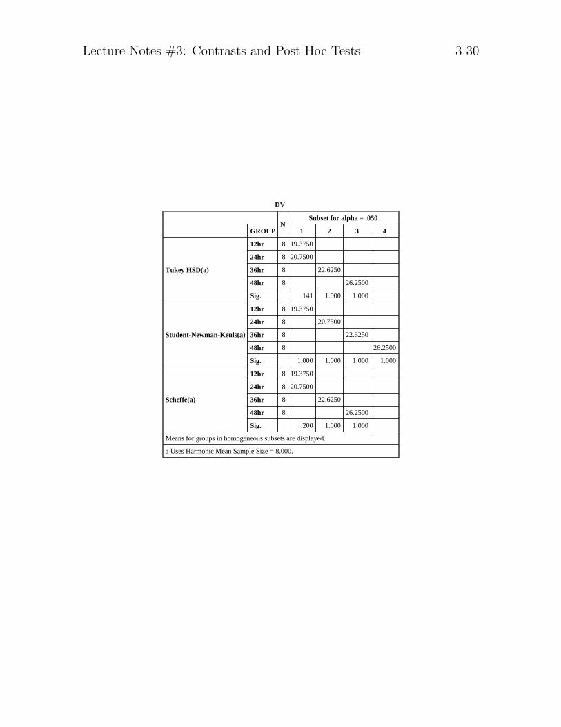
DV
NSubset for alpha = .050
GROUP 1 2 3 4
Tukey HSD(a)
12hr 8 19.3750
24hr 8 20.7500
36hr 8 22.6250
48hr 8 26.2500
Sig. .141 1.000 1.000
Student-Newman-Keuls(a)
12hr 8 19.3750
24hr 8 20.7500
36hr 8 22.6250
48hr 8 26.2500
Sig. 1.000 1.000 1.000 1.000
Scheffe(a)
12hr 8 19.3750
24hr 8 20.7500
36hr 8 22.6250
48hr 8 26.2500
Sig. .200 1.000 1.000
Means for groups in homogeneous subsets are displayed.
a Uses Harmonic Mean Sample Size = 8.000.

Lecture Notes #3: Contrasts and Post Hoc Tests 3-31
EXAMPLE OF TUKEY’S W USING SLEEP DEPRIVATION DATA (ALTERNATE OUTPUT)
TUKEY-HSD PROCEDURE
RANGES FOR THE 0.050 LEVEL -
3.86 3.86 3.86
THE RANGES ABOVE ARE TABLE RANGES.
THE VALUE ACTUALLY COMPARED WITH MEAN(J)-MEAN(I) IS..
0.8737 * RANGE * DSQRT(1/N(I) + 1/N(J))
(*) DENOTES PAIRS OF GROUPS SIGNIFICANTLY DIFFERENT AT THE 0.050 LEVEL
G G G G
r r r r
p p p p
Mean Group 1 2 3 4
19.3750 Grp 1
20.7500 Grp 2
22.6250 Grp 3 * *
26.2500 Grp 4 * * *
HOMOGENEOUS SUBSETS (SUBSETS OF GROUPS, WHOSE HIGHEST AND LOWEST MEANS
DO NOT DIFFER BY MORE THAN THE SHORTEST
SIGNIFICANT RANGE FOR A SUBSET OF THAT SIZE)
SUBSET 1
GROUP Grp 1 Grp 2
MEAN 19.3750 20.7500
- - - - - - - - - - - - - - - - -
SUBSET 2
GROUP Grp 3
MEAN 22.6250
- - - - - - - - - -
SUBSET 3
GROUP Grp 4
MEAN 26.2500
- - - - - - - - - -

Lecture Notes #3: Contrasts and Post Hoc Tests 3-32
EXAMPLE SHOWING SNK TEST USING THE SLEEP DEPRIVATION DATA (ALTERNATE OUTPUT)
STUDENT-NEWMAN-KEULS PROCEDURE
RANGES FOR THE 0.050 LEVEL -
2.90 3.49 3.86
THE RANGES ABOVE ARE TABLE RANGES.
THE VALUE ACTUALLY COMPARED WITH MEAN(J)-MEAN(I) IS..
0.8737 * RANGE * DSQRT(1/N(I) + 1/N(J))
(*) DENOTES PAIRS OF GROUPS SIGNIFICANTLY DIFFERENT AT THE 0.050 LEVEL
G G G G
r r r r
p p p p
Mean Group 1 2 3 4
19.3750 Grp 1
20.7500 Grp 2 *
22.6250 Grp 3 * *
26.2500 Grp 4 * * *
HOMOGENEOUS SUBSETS (SUBSETS OF GROUPS, WHOSE HIGHEST AND LOWEST MEANS
DO NOT DIFFER BY MORE THAN THE SHORTEST
SIGNIFICANT RANGE FOR A SUBSET OF THAT SIZE)
SUBSET 1
GROUP Grp 1
MEAN 19.3750
- - - - - - - - - -
SUBSET 2
GROUP Grp 2
MEAN 20.7500
- - - - - - - - - -
SUBSET 3
GROUP Grp 3
MEAN 22.6250
- - - - - - - - - -
SUBSET 4
GROUP Grp 4
MEAN 26.2500
Lecture Notes #3: Contrasts and Post Hoc Tests 3-33
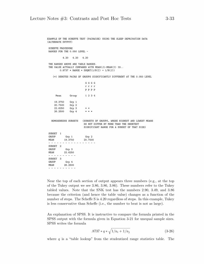
EXAMPLE OF THE SCHEFFE TEST (PAIRWISE) USING THE SLEEP DEPRIVATION DATA
(ALTERNATE OUTPUT)
SCHEFFE PROCEDURE
RANGES FOR THE 0.050 LEVEL -
4.20 4.20 4.20
THE RANGES ABOVE ARE TABLE RANGES.
THE VALUE ACTUALLY COMPARED WITH MEAN(J)-MEAN(I) IS..
0.8737 * RANGE * DSQRT(1/N(I) + 1/N(J))
(*) DENOTES PAIRS OF GROUPS SIGNIFICANTLY DIFFERENT AT THE 0.050 LEVEL
G G G G
r r r r
p p p p
Mean Group 1 2 3 4
19.3750 Grp 1
20.7500 Grp 2
22.6250 Grp 3 * *
26.2500 Grp 4 * * *
HOMOGENEOUS SUBSETS (SUBSETS OF GROUPS, WHOSE HIGHEST AND LOWEST MEANS
DO NOT DIFFER BY MORE THAN THE SHORTEST
SIGNIFICANT RANGE FOR A SUBSET OF THAT SIZE)
SUBSET 1
GROUP Grp 1 Grp 2
MEAN 19.3750 20.7500
- - - - - - - - - - - - - - - - -
SUBSET 2
GROUP Grp 3
MEAN 22.6250
- - - - - - - - - -
SUBSET 3
GROUP Grp 4
MEAN 26.2500
- - - - - - - - - -
Near the top of each section of output appears three numbers (e.g., at the topof the Tukey output we see 3.86, 3.86, 3.86). These numbers refer to the Tukeytabled values. Note that the SNK test has the numbers 2.90, 3.49, and 3.86because the criterion (and hence the table value) changes as a function of thenumber of steps. The Scheffe S is 4.20 regardless of steps. In this example, Tukeyis less conservative than Scheffe (i.e., the number to beat is not as large).
An explanation of SPSS. It is instructive to compare the formula printed in theSPSS output with the formula given in Equation 3-21 for unequal sample sizes.SPSS writes the formula
.8737 ∗ q ∗√
1/ni + 1/nj (3-26)
where q is a “table lookup” from the studentized range statistics table. The
Lecture Notes #3: Contrasts and Post Hoc Tests 3-34
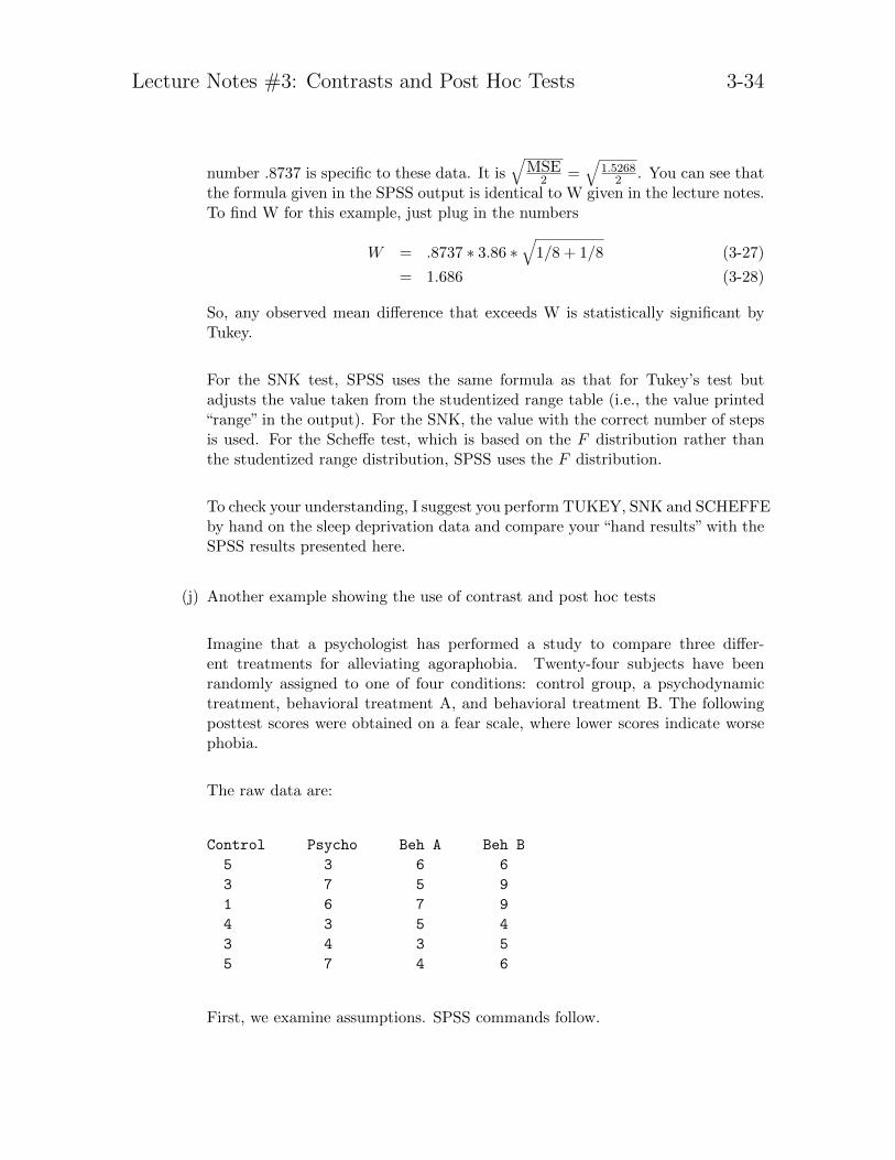
number .8737 is specific to these data. It is√
MSE2 =
√1.5268
2 . You can see thatthe formula given in the SPSS output is identical to W given in the lecture notes.To find W for this example, just plug in the numbers
W = .8737 ∗ 3.86 ∗√
1/8 + 1/8 (3-27)
= 1.686 (3-28)
So, any observed mean difference that exceeds W is statistically significant byTukey.
For the SNK test, SPSS uses the same formula as that for Tukey’s test butadjusts the value taken from the studentized range table (i.e., the value printed“range” in the output). For the SNK, the value with the correct number of stepsis used. For the Scheffe test, which is based on the F distribution rather thanthe studentized range distribution, SPSS uses the F distribution.
To check your understanding, I suggest you perform TUKEY, SNK and SCHEFFEby hand on the sleep deprivation data and compare your “hand results” with theSPSS results presented here.
(j) Another example showing the use of contrast and post hoc tests
Imagine that a psychologist has performed a study to compare three differ-ent treatments for alleviating agoraphobia. Twenty-four subjects have beenrandomly assigned to one of four conditions: control group, a psychodynamictreatment, behavioral treatment A, and behavioral treatment B. The followingposttest scores were obtained on a fear scale, where lower scores indicate worsephobia.
The raw data are:
Control Psycho Beh A Beh B
5 3 6 6
3 7 5 9
1 6 7 9
4 3 5 4
3 4 3 5
5 7 4 6
First, we examine assumptions. SPSS commands follow.

Lecture Notes #3: Contrasts and Post Hoc Tests 3-35
data list file = ’data.clinic’ free / treat fear
value labels treat 1 ’control’ 2 ’psycho’ 3 ’beh A’ 4 ’beh B’
examine variables fear by treat/plot boxplot npplot.
I’ll only show the boxplots in the interest of space. You can generate the normalplots on your own.
6666N =
TREAT
beh Bbeh Apsychocontrol
FE
AR
10
8
6
4
2
0
The equality of variance assumption appears satisfied, though difficult to tell withonly six subjects per cell. No extreme outliers are evident. Symmetry seems okaytoo.
Next, examine the structural model and parameter estimates.
Yij = µ+ αi + εij (3-29)
The parameter estimates are easy to calculate. All you need are the cell meansand the grand mean. Be careful that the grand mean is the“real”grand mean (themean of the cell means rather than the mean of all the data). This informationappears in several places in the SPSS output (i.e., you’ll get it when you askfor boxplots, and if you use the /statistics = descriptives subcommand inONEWAY, you can ask for MEANS = tables fear by treat.) Below Iinclude the output from the MEANS command.
means tables = fear by treat.

Lecture Notes #3: Contrasts and Post Hoc Tests 3-36
Variable Value Label Mean Std Dev Cases Parameter est.
For Entire Population 5.0000 1.9560 24 µ = 5
TREAT 1.00 control 3.5000 1.5166 6 α1 = Y1 − µ = −1.5TREAT 2.00 psycho 5.0000 1.8974 6 α2 = Y2 − µ = 0TREAT 3.00 beh A 5.0000 1.4142 6 α3 = Y3 − µ = 0TREAT 4.00 beh B 6.5000 2.0736 6 α4 = Y4 − µ = 1.5
We can see that the psychodynamic and beh A groups had treatment effects ofzero; the two remaining groups had treatment effects of 1.5 (note sign).
Next we run the inferential tests: ANOVA & contrasts
I’ll use the ONEWAY command for the overall ANOVA, contrasts, and post hoctests. Note that with only six subjects per cell we shouldn’t be too optimisticthat this study will lead to significant results. Usually, effect sizes are smallenough that six subjects per cell doesn’t give one much power.
oneway fear by treat/statistics all/contrasts = -3, 1, 1, 1/contrasts = 0, -2, 1, 1/contrasts = 0, 0, 1, -1/ranges=tukey.
ANALYSIS OF VARIANCE
SUM OF MEAN F F
SOURCE D.F. SQUARES SQUARES RATIO PROB.
BETWEEN GROUPS 3 27.0000 9.0000 2.9508 .0575
WITHIN GROUPS 20 61.0000 3.0500
TOTAL 23 88.0000
This ANOVA tells us that the omnibus test is not statistically significant atα = 0.05. That is, the four means are not different from each other. But thistest is not very informative as to where the differences could be (if there wereany) because it is examining the four means as a set.
We need to be careful because there are only six subjects per cell so this is nota powerful test.

Lecture Notes #3: Contrasts and Post Hoc Tests 3-37
The design calls for a natural set of contrasts. Make sure you understand whythese three contrasts provide a natural set of comparisons for this particularstudy. These three contrasts are orthogonal.
CONTRAST COEFFICIENT MATRIX
Grp 1 Grp 3
Grp 2 Grp 4
CONTRAST 1 -3.0 1.0 1.0 1.0
CONTRAST 2 0.0 -2.0 1.0 1.0
CONTRAST 3 0.0 0.0 1.0 -1.0
POOLED VARIANCE ESTIMATE
VALUE S. ERROR T VALUE D.F. T PROB.
CONTRAST 1 6.0000 2.4698 2.429 20.0 0.025
CONTRAST 2 1.5000 1.7464 0.859 20.0 0.401
CONTRAST 3 -1.5000 1.0083 -1.488 20.0 0.152
SEPARATE VARIANCE ESTIMATE
VALUE S. ERROR T VALUE D.F. T PROB.
CONTRAST 1 6.0000 2.2583 2.657 10.1 0.024
CONTRAST 2 1.5000 1.8574 0.808 9.3 0.439
CONTRAST 3 -1.5000 1.0247 -1.464 8.8 0.178
Next, I perform a 95% CI on Contrast #1 to illustrate the computation. Fromthe output we see that I = 6 and se(I) = 2.47. The t-value for a 95% CI with20 degrees of freedom is 2.086 (from the t-table). Recall that the formula for aCI on a contrast is
I ± tα/2,df se(I)
6 ± (2.086)(2.47)
6 ± 5.15
yielding the interval (0.85, 11.15). This interval does not contain zero.
Multiplicity of tests
One could merely report these three contrast values and corresponding t values.That would be fine. But the problem of multiplicity is present and the researcherwould want to replicate the results. If a replication is not feasible, then onesolution to the multiplicity problem is to use a Bonferroni-type correction tocontrol the experimentwise error rate. Because there are three contrasts, the percomparison α′ will be α
3 = 0.017. None of the three contrasts are now significantbecause 0.017 is the tail probability to beat, not 0.05. Note that the Bonferronicorrection involves only a change in the criterion for what is deemed “statistically

Lecture Notes #3: Contrasts and Post Hoc Tests 3-38
significant”—no other computational changes are necessary when implementingthe Bonferroni correction.
Post hoc tests
Let’s imagine that the researcher didn’t have any hypotheses whatsoever. Astrange statement given the specifics of the study. Because the researcher ison a fishing expedition, then post hoc tests would be appropriate. Here I showall possible pair-wise comparisons using Tukey’s Honestly Significant Differenceprocedure.
POST HOC TEST (ALL POSSIBLE PAIRWISE COMPARISONS)
TUKEY-HSD PROCEDURE
RANGES FOR THE 0.050 LEVEL -
3.95 3.95 3.95
THE RANGES ABOVE ARE TABLE RANGES.
THE VALUE ACTUALLY COMPARED WITH MEAN(J)-MEAN(I) IS..
1.2349 * RANGE * DSQRT(1/N(I) + 1/N(J))
(*) DENOTES PAIRS OF GROUPS SIGNIFICANTLY DIFFERENT AT THE 0.050 LEVEL
G G G G
r r r r
p p p p
Mean Group 1 2 3 4
3.5000 Grp 1
5.0000 Grp 2
5.0000 Grp 3
6.5000 Grp 4 *
HOMOGENEOUS SUBSETS (SUBSETS OF GROUPS, WHOSE HIGHEST AND LOWEST MEANS
DO NOT DIFFER BY MORE THAN THE SHORTEST
SIGNIFICANT RANGE FOR A SUBSET OF THAT SIZE)
SUBSET 1
GROUP Grp 1 Grp 2 Grp 3
MEAN 3.5000 5.0000 5.0000
- - - - - - - - - - - - - - - - - - - - - - - -
SUBSET 2
GROUP Grp 2 Grp 3 Grp 4
MEAN 5.0000 5.0000 6.5000
- - - - - - - - - - - - - - - - - - - - - - - -
I now illustrate the computation of the Tukey test. Using the method for W with

Lecture Notes #3: Contrasts and Post Hoc Tests 3-39
equal n we have
W = qα(T,v)
√MSE
n(3-30)
= 3.95
√3.05
6(3-31)
= 2.82 (3-32)
So any pairwise difference between means that exceeds W=2.82 is statisticallysignificant by Tukey. In this example, only the difference between Group 1 andGroup 4 means exceeds 2.82.
To illustrate the Scheffe test I’ll use the SPSS shortcut that I introduced earlierin these lecture notes. Recall that we setup a new t critical based on the Scheffetest, and we use that new t critical to evaluate the observed t in the contrastportion of the SPSS output. Recall the new t critical is given by
tcritical =√
(T-1)Fα, df1, df2
=√
(4− 1) ∗ 3.098
= 3.049
The tabled F for 3 and 20 degrees of freedom is 3.098. We scan the contrastoutput and look for contrasts that have an observed t that exceeds 3.049. Noneof the contrasts are significant by Scheffe. Note that the usual t criterion for anuncorrected t is a number near 2 (depending on degrees of freedom). The Scheffeis quite conservative at 3.049.
Another equivalent way to compute the Scheffe test is to calculate S, which isthe contrast value to beat. In this example, SPSS computes I and its standarderror. I’ll just illustrate the first contrast in this example. Recall the formula
S =√
V(I)√
(T-1)Fα, df1, df2 (3-33)
= 2.4698 ∗ 3.049 (3-34)
= 7.53 (3-35)
where the 2.4698 is the se printed in the output and the 3.049 is the term Ishowed you how to compute in the previous paragraph. So any observed I thatexceeds 7.53 is statistically significant by Scheffe. None of the observed Is exceed7.53 so, as we saw with the other equivalent methods, none of the three contrastsare statistically significant.
To compute the Welch-like version of the Scheffe just replace df2 (degrees of free-dom for the denominator) with the degrees of freedom reported in the “separate
Lecture Notes #3: Contrasts and Post Hoc Tests 3-40
variance” portion of the SPSS output and use the separate variance estimate ofthe standard error of I (or for the other method, the separate variance observedt). You use this newer degrees of freedom in the table lookup of F.
Why not perform the contrast (1, 0, 0, -1) corresponding to the comparisonbetween control and Behavioral Treatment B? It depends on how you decidedto test this contrast. Did you predict that the only difference would be betweenthe control and Beh B conditions? If so, the you can go ahead and run such acontrast. The contrast would be tested at α = 0.5. What are the remaining twoorthogonal contrasts? If you run those tests, you will need to grapple with themultiplicity problem and need to decide whether or not to perform a Bonferronicorrection.
However, if you look at the data and say, “Gee, that’s interesting. I would havenever guessed that Beh B would have been the only group that would be differentthan the control.” Then you should perform a post hoc test such as Scheffe totake into account chance factors that might have lead to such a result.
(k) Uniqueness of a contrast
Contrasts are unique up to a scale transformation. You get the identical p-valueif you multiply all the contrast weights by a constant real number (positive ornegative). The size of the CI will shrink or expand accordingly, but key features(such as whether or not the CI includes 0 and whether or not the CI overlapswith other contrasts that are on the same scale) remain the same.
Let’s look at Contrast #1 in the previous example. What does the value I = 6mean? It means that 3 times the control group minus the sum of the three treat-ment means equals 6. Some people prefer using contrasts that are normalized sothe sum of the absolute values of the weights equals 2 (i.e.,
∑|a| = 2).
For Contrast #1 above I used the weights (-3, 1, 1, 1). I could have used (-1,13 ,13 ,13) and would have seen an identical p-value. The weights in both contrastsare proportional so they test exactly the same hypothesis. So, I know, withouthaving to use any SPSS commands, that the value of the contrast (-1, 1
3 ,13 ,13) willbe 2 (i.e., 6
3) and the standard error will be 0.8233 (i.e,. 2.46983 ).
To check this (and to convince you by example) here is the SPSS command forthis new contrast. Unfortunately, SPSS does not allow one to enter fractions ascontrast weights so one needs to round off. Let’s see what happens when I enterthe contrast (-1, 0.33, 0.33, 0.34).

Lecture Notes #3: Contrasts and Post Hoc Tests 3-41
data list file = ’data.clinic’ free / treat fear
value labels treat 1 ’control’ 2 ’psycho’ 3 ’beh A’ 4 ’beh B’
oneway fear by treat/statistics all/contrasts = -1, 0.33, 0.33, 0.34.
Grp 1 Grp 3
Grp 2 Grp 4
CONTRAST 1 -1.0 0.3 0.3 0.3
POOLED VARIANCE ESTIMATE
VALUE S. ERROR T VALUE D.F. T PROB.
CONTRAST 1* 2.0100 0.8233 2.441 20.0 0.024
SEPARATE VARIANCE ESTIMATE
S. ERROR T VALUE D.F. T PROB.
0.7535 2.667 10.1 0.023
* ABOVE INDICATES SUM OF COEFFICIENTS IS NOT ZERO.
As we knew already, the contrast value is 2 (roundoff error) and the standarderror is 0.8233. The 95% CI is (the t-value = 2.086 remains the same as before)
I ± tα/2,df se(I)
2 ± (2.086)(0.8233)
2 ± 1.7174
yielding the interval (0.28, 3.72). Note that, as before, zero is not included.
Let’s look at another example showing that contrasts are unique up to a scaletransformation. Using the sleep deprivation data I presented in a previous lec-ture. All three contrasts are identical and yield identical p-values; the weightsare proportional.
data list file = name free / id dv codes rdv
value labels codes 1 ’12hr’ 2 ’24hr’ 3 ’36hr’ 4 ’48hr’
oneway dv by codes/contrasts = 1, 1, -2, 0/contrasts = -1, -1, 2, 0/contrasts = .5, .5, -1, 0.
ANALYSIS OF VARIANCE
SUM OF MEAN F F
SOURCE D.F. SQUARES SQUARES RATIO PROB.
BETWEEN GROUPS 3 213.2500 71.0833 46.5575 .0000
WITHIN GROUPS 28 42.7500 1.5268
TOTAL 31 256.0000

Lecture Notes #3: Contrasts and Post Hoc Tests 3-42
Grp 1 Grp 3
Grp 2 Grp 4
CONTRAST 1 1.0 1.0 -2.0 0.0
CONTRAST 2 -1.0 -1.0 2.0 0.0
CONTRAST 3 0.5 0.5 -1.0 0.0
POOLED VARIANCE ESTIMATE
VALUE S. ERROR T VALUE D.F. T PROB.
CONTRAST 1 -5.1250 1.0701 -4.789 28.0 0.000
CONTRAST 2 5.1250 1.0701 4.789 28.0 0.000
CONTRAST 3 -2.5625 0.5350 -4.789 28.0 0.000
SEPARATE VARIANCE ESTIMATE
S. ERROR T VALUE D.F. T PROB.
1.0426 -4.916 14.5 0.000
1.0426 4.916 14.5 0.000
0.5213 -4.916 14.5 0.000

Lecture Notes #3: Contrasts and Post Hoc Tests 3-43
Appendix 1
ANOVA ON SLEEP DEPRIVATION DATA
SPSS SYNTAX:
oneway dv by codes
/contrast 3 -1 -1 -1
/contrast 0 2 -1 -1
/contrast 0 0 1 -1
/contrast 1 0 0 -1.
SUM OF MEAN F F
SOURCE D.F. SQUARES SQUARES RATIO PROB.
BETWEEN GROUPS 3 213.2500 71.0833 46.5575 .0000
WITHIN GROUPS 28 42.7500 1.5268
TOTAL 31 256.0000
CONTRAST COEFFICIENT MATRIX
Grp 1 Grp 3
Grp 2 Grp 4
CONTRAST 1 3.0 -1.0 -1.0 -1.0
CONTRAST 2 0.0 2.0 -1.0 -1.0
CONTRAST 3 0.0 0.0 1.0 -1.0
CONTRAST 4 1.0 0.0 0.0 -1.0
POOLED VARIANCE ESTIMATE
VALUE S. ERROR T VALUE D.F. T PROB.
CONTRAST 1 -11.5000 1.5133 -7.599 28.0 0.000
CONTRAST 2 -7.3750 1.0701 -6.892 28.0 0.000
CONTRAST 3 -3.6250 0.6178 -5.867 28.0 0.000
CONTRAST 4 -6.8750 0.6178 -11.128 28.0 0.000
SEPARATE VARIANCE ESTIMATE
VALUE S. ERROR T VALUE D.F. T PROB.
CONTRAST 1 -11.5000 1.4745 -7.799 12.6 0.000
CONTRAST 2 -7.3750 1.0969 -6.724 13.5 0.000
CONTRAST 3 -3.6250 0.6178 -5.867 13.9 0.000
CONTRAST 4 -6.8750 0.6178 -11.128 13.9 0.000
The pooled variance estimate t values correspond to the formulae in the lecture. The separatevariance estimate is a generalization of Welch’s work to contrasts. Note that the separate varianceestimate “corrects” for violations of the equality of variance assumption by reducing the degrees offreedom.
SSC for contrast 1 is given by (this example has equal sample sizes so the niare equal)
SSC1 =I2
∑ a2
ini
=[(3)Y1 + (-1)Y2 + (-1)Y3 + (-1)Y4]2∑ (3)2+(−1)2+(−1)2+(−1)2
n
=[(3)19.375 + (−1)20.75 + (−1)22.625 + (−1)26.25]2
128
= 88.167

Lecture Notes #3: Contrasts and Post Hoc Tests 3-44
Similarly, we can compute
SSC2 = 72.52
SSC3 = 52.56
SSC4 = 188.79
Note that SSB = SSC1 + SSC2 + SSC3. So what about SSC4? It is not orthogonal with the otherthree contrasts and is consequently redundant. Note that SSC4 accounts for quite a hefty chunk ofthe SSB.
Here is a source table reflecting the decomposition of SSB into the separate SSC.
SHOW BREAKDOWN OF SSB WITHIN THE ANOVA TABLE
SUM OF MEAN F t
SOURCE D.F. SQUARES SQUARES RATIO value
BETWEEN GROUPS 3 213.2500 71.0833 46.5575
CONTRAST 1 1 88.17 88.02 57.65 7.59
CONTRAST 2 1 72.52 72.52 47.49 6.89
CONTRAST 3 1 52.56 52.56 34.42 5.87
WITHIN GROUPS 28 42.7500 1.5268
TOTAL 31 256.0000
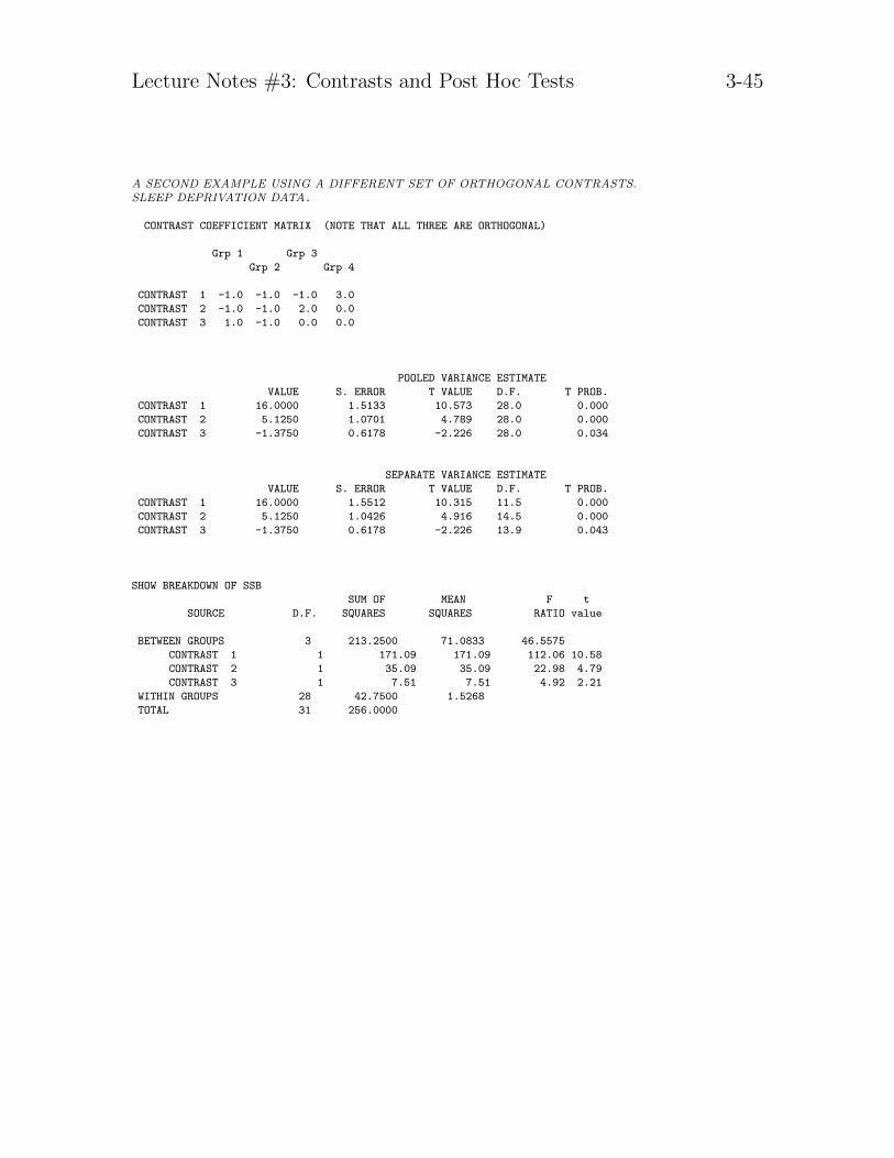
Lecture Notes #3: Contrasts and Post Hoc Tests 3-45
A SECOND EXAMPLE USING A DIFFERENT SET OF ORTHOGONAL CONTRASTS.SLEEP DEPRIVATION DATA.
CONTRAST COEFFICIENT MATRIX (NOTE THAT ALL THREE ARE ORTHOGONAL)
Grp 1 Grp 3
Grp 2 Grp 4
CONTRAST 1 -1.0 -1.0 -1.0 3.0
CONTRAST 2 -1.0 -1.0 2.0 0.0
CONTRAST 3 1.0 -1.0 0.0 0.0
POOLED VARIANCE ESTIMATE
VALUE S. ERROR T VALUE D.F. T PROB.
CONTRAST 1 16.0000 1.5133 10.573 28.0 0.000
CONTRAST 2 5.1250 1.0701 4.789 28.0 0.000
CONTRAST 3 -1.3750 0.6178 -2.226 28.0 0.034
SEPARATE VARIANCE ESTIMATE
VALUE S. ERROR T VALUE D.F. T PROB.
CONTRAST 1 16.0000 1.5512 10.315 11.5 0.000
CONTRAST 2 5.1250 1.0426 4.916 14.5 0.000
CONTRAST 3 -1.3750 0.6178 -2.226 13.9 0.043
SHOW BREAKDOWN OF SSB
SUM OF MEAN F t
SOURCE D.F. SQUARES SQUARES RATIO value
BETWEEN GROUPS 3 213.2500 71.0833 46.5575
CONTRAST 1 1 171.09 171.09 112.06 10.58
CONTRAST 2 1 35.09 35.09 22.98 4.79
CONTRAST 3 1 7.51 7.51 4.92 2.21
WITHIN GROUPS 28 42.7500 1.5268
TOTAL 31 256.0000

Lecture Notes #3: Contrasts and Post Hoc Tests 3-46
A THIRD EXAMPLE USING A DIFFERENT SET OF ORTHOGONAL CONTRASTS (POLYNOMIAL).
CONTRAST COEFFICIENT MATRIX (NOTE THAT ALL THREE ARE ORTHOGONAL)
Grp 1 Grp 3
Grp 2 Grp 4
CONTRAST 1 -3.0 -1.0 1.0 3.0
CONTRAST 2 1.0 -1.0 -1.0 1.0
CONTRAST 3 -1.0 3.0 -3.0 1.0
POOLED VARIANCE ESTIMATE
VALUE S. ERROR T VALUE D.F. T PROB.
CONTRAST 1 22.5000 1.9537 11.517 28.0 0.000
CONTRAST 2 2.2500 0.8737 2.575 28.0 0.016
CONTRAST 3 1.2500 1.9537 0.640 28.0 0.527
SEPARATE VARIANCE ESTIMATE
VALUE S. ERROR T VALUE D.F. T PROB.
CONTRAST 1 22.5000 1.9537 11.517 17.0 0.000
CONTRAST 2 2.2500 0.8737 2.575 27.8 0.016
CONTRAST 3 1.2500 1.9537 0.640 17.0 0.531
SHOW BREAKDOWN OF SSB
SUM OF MEAN F t
SOURCE D.F. SQUARES SQUARES RATIO value
BETWEEN GROUPS 3 213.2500 71.0833 46.5575
CONTRAST 1 1 202.32 202.32 132.58 11.51
CONTRAST 2 1 10.13 10.13 6.63 2.57
CONTRAST 3 1 0.61 0.61 0.40 0.63
WITHIN GROUPS 28 42.7500 1.5268
TOTAL 31 256.0000

Lecture Notes #3: Contrasts and Post Hoc Tests 3-47
Appendix 2
ALL PAIRWISE COMPARISONS OF THE FOUR GROUPS IN THE SLEEP DEPRIVATION STUDY
CONTRAST COEFFICIENT MATRIX
Grp 1 Grp 3
Grp 2 Grp 4
CONTRAST 1 1.0 -1.0 0.0 0.0
CONTRAST 2 1.0 0.0 -1.0 0.0
CONTRAST 3 1.0 0.0 0.0 -1.0
CONTRAST 4 0.0 1.0 -1.0 0.0
CONTRAST 5 0.0 1.0 0.0 -1.0
CONTRAST 6 0.0 0.0 1.0 -1.0
POOLED VARIANCE ESTIMATE
VALUE S. ERROR T VALUE D.F. T PROB.
CONTRAST 1 -1.3750 0.6178 -2.226 28.0 0.034
CONTRAST 2 -3.2500 0.6178 -5.260 28.0 0.000
CONTRAST 3 -6.8750 0.6178 -11.128 28.0 0.000
CONTRAST 4 -1.8750 0.6178 -3.035 28.0 0.005
CONTRAST 5 -5.5000 0.6178 -8.902 28.0 0.000
CONTRAST 6 -3.6250 0.6178 -5.867 28.0 0.000
SEPARATE VARIANCE ESTIMATE
VALUE S. ERROR T VALUE D.F. T PROB.
CONTRAST 1 -1.3750 0.6178 -2.226 13.9 0.043
CONTRAST 2 -3.2500 0.5939 -5.473 14.0 0.000
CONTRAST 3 -6.8750 0.6178 -11.128 13.9 0.000
CONTRAST 4 -1.8750 0.6178 -3.035 13.9 0.009
CONTRAST 5 -5.5000 0.6409 -8.582 14.0 0.000
CONTRAST 6 -3.6250 0.6178 -5.867 13.9 0.000
Recall that the sums of squares for each contrasts is given by
SSCi =I2∑ a2
ini
(3-36)
Note that for all these contrasts the denominator of Equation 3-36 is 0.25. The numerator is simply the “value” of thecontrast squared.
The sums of squares for each contrast pairwise contrast are
SSC1 = 7.6
SSC2 = 42.2
SSC3 = 188.8
SSC4 = 14.1
SSC5 = 121.0
SSC6 = 52.6

Lecture Notes #3: Contrasts and Post Hoc Tests 3-48
Appendix 3: R syntax
There are many ways to test contrasts and post-hoc tests in R. For some of the remaining lecturenotes I’ll put most of the R syntax in an appendix because the discussion becomes very specializedand more about R than about statistics. I’ll also work in some common R errors in the discussion,as I do below in the case of incorrectly using the aov() command without a grouping code that isspecifically defined as a factor.
Here I list a few of the basics. First, read data, label columns, create data.frame.
> sleep.data <- read.table("/Users/gonzo/rich/Teach/Gradst~1/unixfiles/lectnotes/lect3/data.sleep2")
> names(sleep.data) <- c("subject", "performance","group", "residual")
> sleep.data <- data.frame(sleep.data)
Run regular ANOVA, just prints the omnibus F test, no contrasts by default.
> summary(aov(performance ~ group, data=sleep.data))
Df Sum Sq Mean Sq F value Pr(>F)
group 1 202.5 202.50 113.6 1.02e-11 ***
Residuals 30 53.5 1.78
---
Signif. codes: 0 ‘***’ 0.001 ‘**’ 0.01 ‘*’ 0.05 ‘.’ 0.1 ‘ ’ 1
Do you see something wrong with this source table? There are four levels of the group factor sothere should be 3 degrees of freedom for between groups, but the output lists 1 degree of freedom.The problem is that R does not know that group is a factor; it interpreted the colulmn labeled groupas the numbers 1 to 4 rather than labels denoting four groups. We need to define factors explicitly;let’s try that again.
> sleep.data$group <- factor(sleep.data$group)
> summary(aov(performance ~ group, data=sleep.data))
Df Sum Sq Mean Sq F value Pr(>F)
group 3 213.25 71.08 46.56 5.22e-11 ***
Residuals 28 42.75 1.53
---
Signif. codes: 0 ‘***’ 0.001 ‘**’ 0.01 ‘*’ 0.05 ‘.’ 0.1 ‘ ’ 1
These kinds of silly errors illustrate why it is important to know what you expect to see (such as

Lecture Notes #3: Contrasts and Post Hoc Tests 3-49
the degrees of freedom) before running the command so you can spot errors. If you aren’t carefulyou can end up publishing incorrect analyses, and unfortunately there are many such examples inthe literature.
You can define contrasts directly in a factor. So if we have a grouping variable with four levels forContrasts in R
the sleep deprivation example we first define group variable as a factor and then define an orthogonalset of contrasts for that factor. The benefit of this approach is that as you call that factor in variouscommands the “contrast structure” follows the variable and you don’t have to keep respecifyingthe contrasts. For example, if I want to test say the orthogonal set of three contrasts, c(1,-1,0,0),c(1,1,-2,0), and c(1,1,1,-3), the following two commands will do the trick.
> contrasts(sleep.data$group) <- cbind(C12.24=c(1,-1,0,0),
+ C1224.36=c(1,1,-2,0), C122436.48=c(1,1,1,-3))
> #check the command worked as intended
> contrasts(sleep.data$group)
C12.24 C1224.36 C122436.48
1 1 1 1
2 -1 1 1
3 0 -2 1
4 0 0 -3
> anova.output <- aov(performance ~ group, data=sleep.data,contrasts=contrasts(sleep.data$group))
> summary(anova.output, split=list(group= list(C12.24=1,C1224.36=2,C122436.48=3)))
Df Sum Sq Mean Sq F value Pr(>F)
group 3 213.25 71.08 46.558 5.22e-11 ***
group: C12.24 1 7.56 7.56 4.953 0.0343 *
group: C1224.36 1 35.02 35.02 22.938 4.93e-05 ***
group: C122436.48 1 170.67 170.67 111.782 2.78e-11 ***
Residuals 28 42.75 1.53
---
Signif. codes: 0 ‘***’ 0.001 ‘**’ 0.01 ‘*’ 0.05 ‘.’ 0.1 ‘ ’ 1
The syntax of the last line is interpreted as split the output of anova.output into the first, secondand third contrasts that are defined in the factor(group). That’s a lot of typing and I generally avoidthe aov() command for reasons that I’ll go into in LN4 due to the way the aov() treats factorialdesigns with unequal sample sizes. Note that this output is not in the form of the usual contrastvalue, se, t and p but rather in terms of the decomposition of the sum of squares (think pie chart).If you want to report the t rather than the F, just take the sqrt of the F.
> sqrt(4.953)

Lecture Notes #3: Contrasts and Post Hoc Tests 3-50
[1] 2.225534
> sqrt(22.938)
[1] 4.789363
> sqrt(111.782)
[1] 10.5727
We can do this because for F’s with one degree of freedom in the numerator (all contrasts have onenumerator df), we can use the relation that F 2 = t, the pvalues will be the same, etc.
Some R commands like lm() will use this contrast information in the factor and organize the outputaccordingly; this is the version I usually use because it is so simple and the output is in terms ofthe familiar contrast value, se, t and p. But for now you should only use it for orthogonal sets ofcontrasts as I show below.
> output.lm <- lm(performance ~ group, sleep.data)
> summary(output.lm)
Call:
lm(formula = performance ~ group, data = sleep.data)
Residuals:
Min 1Q Median 3Q Max
-2.3750 -0.6562 0.0000 0.6562 2.3750
Coefficients:
Estimate Std. Error t value Pr(>|t|)
(Intercept) 22.2500 0.2184 101.863 < 2e-16 ***
groupC12.24 -0.6875 0.3089 -2.226 0.0343 *
groupC1224.36 -0.8542 0.1783 -4.789 4.93e-05 ***
groupC122436.48 -1.3333 0.1261 -10.573 2.78e-11 ***
---
Signif. codes: 0 ‘***’ 0.001 ‘**’ 0.01 ‘*’ 0.05 ‘.’ 0.1 ‘ ’ 1
Residual standard error: 1.236 on 28 degrees of freedom
Multiple R-squared: 0.833, Adjusted R-squared: 0.8151
F-statistic: 46.56 on 3 and 28 DF, p-value: 5.222e-11

Lecture Notes #3: Contrasts and Post Hoc Tests 3-51
The t from the lm() command is identical to the sqrt of the F from the aov() command above.
You can get the source table from the output of the lm() command through the anova() command
> anova(output.lm)
Analysis of Variance Table
Response: performance
Df Sum Sq Mean Sq F value Pr(>F)
group 3 213.25 71.083 46.557 5.222e-11 ***
Residuals 28 42.75 1.527
---
Signif. codes: 0 ‘***’ 0.001 ‘**’ 0.01 ‘*’ 0.05 ‘.’ 0.1 ‘ ’ 1
You can also test contrasts directly using the fit.contrast() command in the library(gmodels). Thisis probably the one you should use for now because it works for both orthogonal and nonorthogonalcontrasts.
> library(gmodels)
> out.model <- aov(performance~group,sleep.data)
> fit.contrast(out.model,"group",c(1,-1,0,0),df=T,conf.int=.95,show.all=T)
Estimate Std. Error t value Pr(>|t|) DF lower CI
group c=( 1 -1 0 0 ) -1.375 0.6178159 -2.225582 0.03427037 28 -2.640538
upper CI
group c=( 1 -1 0 0 ) -0.1094616
> #or if you want an entire orthogonal set
> fit.contrast(out.model,"group",rbind("12v24"=c(1,-1,0,0),
+ "36v(12+24)"=c(1,1,-2,0), "48vall"=c(1,1,1,-3)))
Estimate Std. Error t value Pr(>|t|)
group12v24 -1.375 0.6178159 -2.225582 3.427037e-02
group36v(12+24) -5.125 1.0700884 -4.789324 4.933506e-05
group48vall -16.000 1.5133336 -10.572685 2.775713e-11
>
>

Lecture Notes #3: Contrasts and Post Hoc Tests 3-52
This output provides estimate, se(est), t and p-value. It is equal to the lm() output and the aov()output above. If you want a column for degrees of freedom, include the argument df=T. You canadd the argument conf.int=.95 to get confidence intervals for the contrast estimates. This commanddoesn’t offer the Welch test though (last time I checked at least) so it only applies when the equalityof variance assumption holds.
The fit.contrast function can also handle nonorthogonal contrasts. But if you choose to use the lm()command with nonorthogonal contrasts be careful because the lm() does something different withnonorthogonal contrasts, which will be explained after we do regression. So be careful if you use lm()with non-orthognoal contrasts. While fit.contrast() can allow non-orthogonal contrasts it is limitedin that there can’t be more than number of groups minus 1 contrasts in a single command, so ifyou want to test more than number of groups minus 1 non-orthogonal contrasts, then run multiplefit.contrast commands.
Let me illustrate. Here is the fit.contrast command for the first 3 contrasts in Appendix 2. Outputfrom the fit.contrast() command matches the pooled contrast version in SPSS. But the lm() versiongives a different answer.
> #first 3 non-orthogonal contrasts
> fit.contrast(out.model,"group",rbind("cont1"=c(1,-1,0,0),
+ "cont2"=c(1,0,-1,0), "cont3"=c(1,0,0,-1)))
Estimate Std. Error t value Pr(>|t|)
groupcont1 -1.375 0.6178159 -2.225582 3.427037e-02
groupcont2 -3.250 0.6178159 -5.260467 1.361059e-05
groupcont3 -6.875 0.6178159 -11.127911 8.644137e-12
> #output matches appendix 2 first three contrasts
>
> #lm version
> contrasts(sleep.data$group) <- cbind(C1=c(1,-1,0,0),
+ C2=c(1,0,-1,0), C3=c(1,0,0,-1))
> #check the command worked as intended
> contrasts(sleep.data$group)
C1 C2 C3
1 1 1 1
2 -1 0 0
3 0 -1 0
4 0 0 -1
> output.lm <- lm(performance ~ group, sleep.data)
> summary(output.lm)

Lecture Notes #3: Contrasts and Post Hoc Tests 3-53
Call:
lm(formula = performance ~ group, data = sleep.data)
Residuals:
Min 1Q Median 3Q Max
-2.3750 -0.6562 0.0000 0.6562 2.3750
Coefficients:
Estimate Std. Error t value Pr(>|t|)
(Intercept) 22.2500 0.2184 101.863 < 2e-16 ***
groupC1 1.5000 0.3783 3.965 0.000462 ***
groupC2 -0.3750 0.3783 -0.991 0.330082
groupC3 -4.0000 0.3783 -10.573 2.78e-11 ***
---
Signif. codes: 0 ‘***’ 0.001 ‘**’ 0.01 ‘*’ 0.05 ‘.’ 0.1 ‘ ’ 1
Residual standard error: 1.236 on 28 degrees of freedom
Multiple R-squared: 0.833, Adjusted R-squared: 0.8151
F-statistic: 46.56 on 3 and 28 DF, p-value: 5.222e-11
> #t.tests are not the same as with SPSS nor fit.contrast; yikes
>
These alternative methods can lead to different conclusions. One needs to be careful about what oneis doing and make sure the correct commands are being tested; don’t just assume you can extend acommand if you don’t understand what you are doing. Here fit.contrast() produces the correct testsbut lm() doesn’t unless you do the contrasts correctly.
If you want to know how to get lm() to produce the right output for now you need to apply a differentset of contrasts that involves the inverse of the transpose (that’s matrix algebra terminology thatwe will cover next term). I illustrate here with the first three contrasts in Appendix 2 that didn’treproduce correctly in the lm() command earlier but now we can get them reproduced correctly.
> #write the contrast matrix you want
> contmat <- cbind(c(1,1,1,1),c(1,-1,0,0),c(1,0,-1,0),c(1,0,0,-1))
> #transform that to a new matrix
> newcontmat <- solve(t(contmat))
> newcontmat
[,1] [,2] [,3] [,4]
[1,] 0.25 0.25 0.25 0.25
[2,] 0.25 -0.75 0.25 0.25
[3,] 0.25 0.25 -0.75 0.25
[4,] 0.25 0.25 0.25 -0.75

Lecture Notes #3: Contrasts and Post Hoc Tests 3-54
> #make the new contrast the one associated with the factor you want to test
> contrasts(sleep.data$group) <- newcontmat[,-1]
> output.lm <- lm(performance ~ group, sleep.data)
> summary(output.lm)
Call:
lm(formula = performance ~ group, data = sleep.data)
Residuals:
Min 1Q Median 3Q Max
-2.3750 -0.6562 0.0000 0.6562 2.3750
Coefficients:
Estimate Std. Error t value Pr(>|t|)
(Intercept) 22.2500 0.2184 101.863 < 2e-16 ***
group1 -1.3750 0.6178 -2.226 0.0343 *
group2 -3.2500 0.6178 -5.260 1.36e-05 ***
group3 -6.8750 0.6178 -11.128 8.64e-12 ***
---
Signif. codes: 0 ‘***’ 0.001 ‘**’ 0.01 ‘*’ 0.05 ‘.’ 0.1 ‘ ’ 1
Residual standard error: 1.236 on 28 degrees of freedom
Multiple R-squared: 0.833, Adjusted R-squared: 0.8151
F-statistic: 46.56 on 3 and 28 DF, p-value: 5.222e-11
Look at the terms in the newcontmat. In order to test the (1, -1, 0, 0) contrast in the lm regressioncommand we need to run the (.25, -.75, .25, .25) contrast. Weird now, but it will make sense laterin the term. Even the coefficients of the regression are identical to the SPSS output even thougha different set of contrasts was conducted. You may want to use the fit.contrast command for nowrather than the lm() command when testing nonorthogonal contrasts until we get to those morecomplicated concepts.
For now: the inverse(transpose()) operation sets up the analysis so that contrasts multiplying theIhats (equivalent to the regression betas) give rise to the cell means. For orthogonal sets of contraststhe inverse is equal to the transpose so returns the original orthogonal matrix of contrasts.
The model.tables command is useful. Once you run the aov() command you use the model.tablescommand to get tables of means or tables of the structural model values.
> out.model <- aov(performance~group,data=sleep.data)
> model.tables(out.model,"effects")
Tables of effects
group
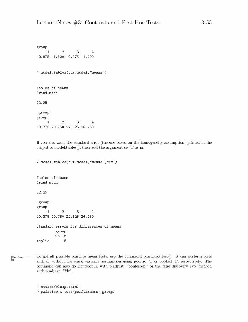
Lecture Notes #3: Contrasts and Post Hoc Tests 3-55
group
1 2 3 4
-2.875 -1.500 0.375 4.000
> model.tables(out.model,"means")
Tables of means
Grand mean
22.25
group
group
1 2 3 4
19.375 20.750 22.625 26.250
If you also want the standard error (the one based on the homogeneity assumption) printed in theoutput of model.tables(), then add the argument se=T as in.
> model.tables(out.model,"means",se=T)
Tables of means
Grand mean
22.25
group
group
1 2 3 4
19.375 20.750 22.625 26.250
Standard errors for differences of means
group
0.6178
replic. 8
To get all possible pairwise mean tests, use the command pairwise.t.test(). It can perform testsBonferonni inR with or without the equal variance assumption using pool.sd=T or pool.sd=F, respectively. The
command can also do Bonferonni, with p.adjust=”bonferroni” or the false discovery rate methodwith p.adjust=”fdr”.
> attach(sleep.data)
> pairwise.t.test(performance, group)
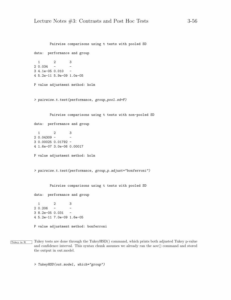
Lecture Notes #3: Contrasts and Post Hoc Tests 3-56
Pairwise comparisons using t tests with pooled SD
data: performance and group
1 2 3
2 0.034 - -
3 4.1e-05 0.010 -
4 5.2e-11 5.9e-09 1.0e-05
P value adjustment method: holm
> pairwise.t.test(performance, group,pool.sd=F)
Pairwise comparisons using t tests with non-pooled SD
data: performance and group
1 2 3
2 0.04309 - -
3 0.00025 0.01792 -
4 1.6e-07 3.0e-06 0.00017
P value adjustment method: holm
> pairwise.t.test(performance, group,p.adjust="bonferroni")
Pairwise comparisons using t tests with pooled SD
data: performance and group
1 2 3
2 0.206 - -
3 8.2e-05 0.031 -
4 5.2e-11 7.0e-09 1.6e-05
P value adjustment method: bonferroni
Tukey tests are done through the TukeyHSD() command, which prints both adjusted Tukey p-valueTukey in R
and confidence interval. This syntax chunk assumes we already ran the aov() command and storedthe output in out.model.
> TukeyHSD(out.model, which="group")

Lecture Notes #3: Contrasts and Post Hoc Tests 3-57
Tukey multiple comparisons of means
95% family-wise confidence level
Fit: aov(formula = performance ~ group, data = sleep.data)
$group
diff lwr upr p adj
2-1 1.375 -0.3118298 3.06183 0.1409966
3-1 3.250 1.5631702 4.93683 0.0000768
4-1 6.875 5.1881702 8.56183 0.0000000
3-2 1.875 0.1881702 3.56183 0.0250231
4-2 5.500 3.8131702 7.18683 0.0000000
4-3 3.625 1.9381702 5.31183 0.0000150
There are many other libraries and special functions to test contrasts and post hoc comparisons. Onepackage worth examining is multcomp. Of course, you can write your own functions in R to organizeoutput the way you want it. That allows you to set up a workflow for commonly used analyses thatyou perform. For example, here is a function I wrote that computes the Welch separate variancetest on contrast (paralleling the SPSS ONEWAY separate variance output):
> sepvarcontrast <- function(dv,group,contrast) {
+ means <- c(by(dv,group,mean))
+ vars <- c(by(dv,group,var))
+ ns <- c(by(dv,group,length))
+ ihat <- contrast %*% means
+ t.denominator <- sqrt(contrast^2 %*% (vars/ns))
+ t.welch <- ihat/t.denominator
+ num.contrast <- ifelse(is.null(dim(contrast)),1,dim(contrast)[1])
+ df.welch <- rep(0,num.contrast)
+ if (is.null(dim(contrast))) contrast <- t(as.matrix(contrast))
+ for (i in 1:num.contrast) {
+ num <- (contrast[i,]^2 %*% (vars))^2
+ den <- sum((contrast[i,]^2 * vars)^2 / (ns-1))
+ df.welch[i] <- num/den
+ }
+ p.welch <- 2*(1- pt(abs(t.welch),df.welch))
+ result <- list(ihat=ihat,se.ihat = t.denominator, t.welch=t.welch,
+ df.welch=df.welch, p.welch=p.welch)
+ return(result)
+ }
You call it by giving the function three arguments: dv, group and contrast such as
> sepvarcontrast(sleep.data$performance,sleep.data$group,c(1,-1,0,0))

Lecture Notes #3: Contrasts and Post Hoc Tests 3-58
$ihat
[,1]
[1,] -1.375
$se.ihat
[,1]
[1,] 0.6178159
$t.welch
[,1]
[1,] -2.225582
$df.welch
[1] 13.91955
$p.welch
[,1]
[1,] 0.04308851
The command can take multiple contrasts in the form of a matrix, such as rbind
> sepvarcontrast(sleep.data$performance,sleep.data$group,rbind(c(1,-1,0,0),c(1,1,-2,0),c(1,1,1,-3)))
$ihat
[,1]
[1,] -1.375
[2,] -5.125
[3,] -16.000
$se.ihat
[,1]
[1,] 0.6178159
[2,] 1.0426186
[3,] 1.5512092
$t.welch
[,1]
[1,] -2.225582
[2,] -4.915508
[3,] -10.314534
$df.welch
[1] 13.91955 14.49169 11.51344
$p.welch
[,1]
[1,] 4.308851e-02

Lecture Notes #3: Contrasts and Post Hoc Tests 3-59
[2,] 2.060439e-04
[3,] 3.670147e-07
This duplicates the output in SPSS for the unequal variance contrast tests (see second example inAppendix 1 of these lecture notes). The separate variance contrast code is not elegant but it works.Future versions of the code can check for missing data, accept formula notation, put the output inthe form of table, work with output of either aov() or lm() in the spirit of the fit.contrast() commanddescribed above, do Scheffe corrections, and handle factorial designs. Adding such bells and whistlesis both the great thing about R but also the bad thing (a huge time commitment).
In LN11 I’ll introduce linear algebra and show how to write code that can test contrasts in verygeneral settings (such as mixed factorial ANOVA designs that have between-subject factors andrepeated-measures factors). That may be the general way to handle classic and Welch-type contrastswith and without Scheffe or Bonferroni corrections all in one convenient R function. So more on thisin LN11.
Here is syntax for Scheffe that reproduces the formulae in the lecture notes. This function assumesScheffe in R
you already computed the contrast value I and the standard error of I. Those two numbers areoutput of performing a contrast using the above procedures. Two more arguments are the numberof groups and the degrees of freedom for error. The default is α = .05 but that can be changedthrough the alpha argument. For the degrees of freedom and standard error of I you can enter eitherthe traditional values or the Welch values.
> scheffe <- function(ihat, se.ihat, ngroups, df.error,alpha=.05) {
+ ScheffeFcritical <- (ngroups - 1) * qf(1-alpha,ngroups-1,df.error)
+ Scheffetcritical <- sqrt(ScheffeFcritical)
+ S <- Scheffetcritical*se.ihat
+ result <- list(Scheffetcritical=Scheffetcritical, S=S, lowerCI=ihat-S,
+ upperCI=ihat+S)
+ return(result)
+ }
This simple Scheffe function prints out the Scheffe t critical, the value S and the confidence intervalaround S. For an example, double check that you get the same result of Scheffe t critical and S forthe psychotherapy/behavioral treatment example. For the first contrast the contrast value was 6,the standard error of the contrast was 2.4698, there were 4 groups and 20 degrees of freedom for theerror.
> scheffe(6, 2.4698, 4, 20)
$Scheffetcritical
[1] 3.048799

Lecture Notes #3: Contrasts and Post Hoc Tests 3-60
$S
[1] 7.529923
$lowerCI
[1] -1.529923
$upperCI
[1] 13.52992
The output of this function reproduces the hand computation shown on page 3-39.
In R the Kruskal-Wallis test is computed through the kruskal.test(dv ∼ group) command.Kruskal-Wallisin R
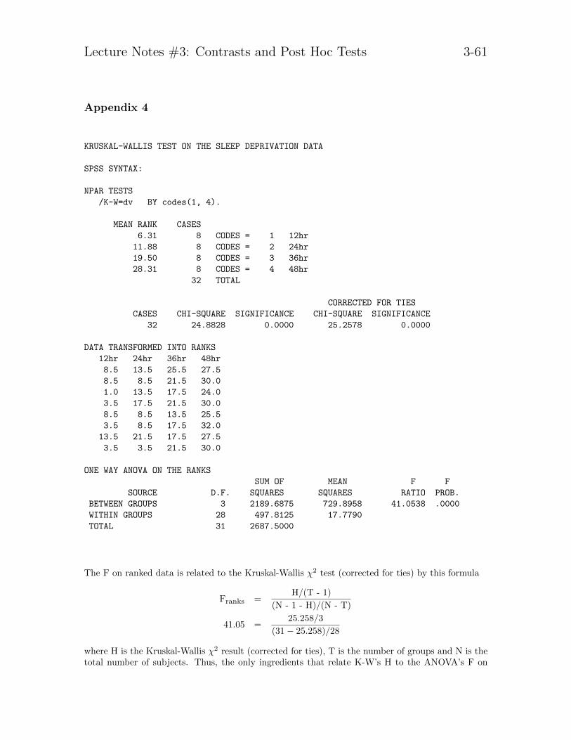
Lecture Notes #3: Contrasts and Post Hoc Tests 3-61
Appendix 4
KRUSKAL-WALLIS TEST ON THE SLEEP DEPRIVATION DATA
SPSS SYNTAX:
NPAR TESTS
/K-W=dv BY codes(1, 4).
MEAN RANK CASES
6.31 8 CODES = 1 12hr
11.88 8 CODES = 2 24hr
19.50 8 CODES = 3 36hr
28.31 8 CODES = 4 48hr
32 TOTAL
CORRECTED FOR TIES
CASES CHI-SQUARE SIGNIFICANCE CHI-SQUARE SIGNIFICANCE
32 24.8828 0.0000 25.2578 0.0000
DATA TRANSFORMED INTO RANKS
12hr 24hr 36hr 48hr
8.5 13.5 25.5 27.5
8.5 8.5 21.5 30.0
1.0 13.5 17.5 24.0
3.5 17.5 21.5 30.0
8.5 8.5 13.5 25.5
3.5 8.5 17.5 32.0
13.5 21.5 17.5 27.5
3.5 3.5 21.5 30.0
ONE WAY ANOVA ON THE RANKS
SUM OF MEAN F F
SOURCE D.F. SQUARES SQUARES RATIO PROB.
BETWEEN GROUPS 3 2189.6875 729.8958 41.0538 .0000
WITHIN GROUPS 28 497.8125 17.7790
TOTAL 31 2687.5000
The F on ranked data is related to the Kruskal-Wallis χ2 test (corrected for ties) by this formula
Franks =H/(T - 1)
(N - 1 - H)/(N - T)
41.05 =25.258/3
(31− 25.258)/28
where H is the Kruskal-Wallis χ2 result (corrected for ties), T is the number of groups and N is thetotal number of subjects. Thus, the only ingredients that relate K-W’s H to the ANOVA’s F on

Lecture Notes #3: Contrasts and Post Hoc Tests 3-62
ranked data are the number of groups (T) and the number of subjects (N). For relatively large N,the p value from the two tests will be indistinguishable.