Lecture Note of Bus 41202, Spring 2012: Value at Risk ...faculty.chicagobooth.edu/ruey.tsay/teaching/bs41202/sp2012/lec9-12.pdf · Lecture Note of Bus 41202, Spring 2012: Value at

Lecture Note of Bus 41202, Spring 2012:

Value at Risk, Expected Shortfall & Risk Management

Classification of Financial Risk

1. Credit risk

2. Market risk

3. Operational risk

We start with the market risk, because

• more high-quality data are available

• easier to understand

• the idea applicable to other types of risk.

What is Value at Risk (VaR)?

• a measure of minimum loss of a financial position within a certain

period of time for a given (small) probability

• the amount a position could decline in a given period, associated

with a given probability (or confidence level)

A formal definition:

• time period given: ∆t = `

• loss in value: L

• CDF of the loss F`(x)

• given (upper tail) probability: p

1

• VaR is defined as

p = Pr[L > VaR] = 1− F`(VaR).

Quantile: xq is the 100qth quantile of the distribution F`(x) if

q = F`(xq), i.e., q = P (L ≤ xq)

and F`(.) is continuous. For discrete distribution, we have

xq = min{x|P (L ≤ x) ≥ q}.

Factors affect VaR:

1. the probability p.

2. the time horizon `.

3. the CDF F`(x). (or CDF of loss)

4. the mark-to-market value of the position.

Remark: Let R(L) be the risk associated with loss L. From a

theoretical point, R(L) must possess the following basic properties:

1. Monotonicity: IfL1 ≤ L2 for all possible outcomes, thenR(L1) ≤R(L2).

2. Sub-additivity: R(L1 +L2) ≤ R(L1) +R(L2) for any two port-

folios.

3. Positive homogeneity: R(hL) = hR(L), where h > 0.

4. Translation invariance: R(L + a) = R(L) + a, where a is a

positive real number.

2

The sub-additivity is associated with risk diversification. The equal-

ity holds when the two portfolios are perfectly positively correlated.

A risk measure is called coherent if it satisfies the above four prop-

erties.

Note. If the loss involved is normally distributed, then VaR is a

coherent risk measure. The sub-additivity can be seen because

(σ1 + σ2)2 = σ21 + σ22 + 2σ1σ2

≥ σ21 + σ22 + 2ρσaσ2

= Var(L1 + L2),

where σ1 and σ2 are the standard errors of L1 and L2, respectively,

and ρ is the correlation between L1 and L2.

However, VaR fails to meet the sub-additive property under certain

conditions. This is the reason that we shall also discuss expected

shortfall or conditional VaR (CVaR), which is a coherent risk mea-

sure. Expected shortfall is the expected loss when the VaR is ex-

ceeded. Some people call expected shortfall as Tail VaR (TVaR)

or expected tail loss (ETL). In the insurance literature, expected

shortfall is called Conditional Tail Expectation or Tail Conditional

Expectation (TCE).

Example of incoherent VaR. See the book of Klugman, Panjer and

Willmot (2008, Wiley). Let Z denote a continuous loss random

variable with the following CDF values

FZ(1) = 0.91, FZ(90) = 0.95, FZ(100) = 0.96.

It is clear that VaR.95(Z) = 90. Now, define loss variables X and Y

such that Z = X + Y , where

X =

Z, if Z ≤ 100

0, if Z > 100,

3

Y =

0, if Z ≤ 100

Z, if Z > 100.

The CDF of X satisfies

FX(1) = .91/.96 ≈ 0.95, FX(90) = 0.95/.96 ≈ 0.99, FX(100) = 1.

Therefore, VaR.95(X) ≈ 1. Turn to Y . The CDF of Y satisfies

FY (0) = 0.96 so that VaR.95(Y ) = 0. Consequently,

VaR.95(X) + VaR.95(Y ) = 1 < VaR.95(Z).

In what follows, we shall use log returns in the analysis (simple re-

turns can also be used).

Why use log returns?

log returns ≈ percentage changes.

VaR = Value × (VaR of log return).

Methods available for market risk

1. RiskMetrics

2. Econometric modeling

3. Empirical quantile

4. Traditional extreme value theory (EVT)

5. EVT based on exceedance over a high threshold

Data used in illustrations:

Daily log returns of IBM stock

• span: July 3, 62 to Dec. 31, 98.

• size: 9190 points

4

Position: long on $10 million.

Note: For a long position, loss occurs at the left (or lower) tail of

the returns. This is equivalent to using the right (or upper) tail if

negative returns are used.

RiskMetrics

• Developed by J.P. Morgan

• rt given Ft−1: N(0, σ2t )

• σ2t follows the special IGARCH(1,1) model

σ2t = βσ2t−1 + (1− β)r2t−1, 1 > β > 0.

• VaR = 1.65σt if p = 0.05. In general, VaR = z1−pσt, where z1−pis the 100(1− p)th quantile of the standard normal distribution.

• k-horizon: VaR[k] =√kVaR

The square root of time rule

• Pros: simplicity and transparence

• Cons: model is not adequate

Example: IBM data

Model:

rt = at, at = σtεt,

σ2t = 0.9595σ2t−1 + (1− 0.9595)a2t−1

Because r9190 = −0.0128 and σ29190 = 0.0003590,

σ29190(1) = 0.0003511.

5

For p = 0.05, VaR of rt = 1.65×√

0.0003511 = 0.03082

VaR = $10, 000, 000× 0.03025 = $308, 200.

For p = 0.01, VaR of rt = 2.3262×√

0.0003511 = 0.04358998, and

VaR = $435,900.

Expected shortfall. From the prior discussion, VaR is simply the

100(1 − p)th quantile of the loss function, where p is the upper tail

probability. When an extreme loss occurs, i.e. VaR is exceeded, the

actual loss can be much higher than VaR. To better quantify the loss

and to employ a coherent risk measure, we consider the expected loss

once the VaR is exceeded. Let q = 1 − p. The expected shortfall

(ES) is then

ESq = E(L|L > VaRq).

For standard Normal distribution, we have ESq = f (VaRq)/p, where

f (x) = 1√2π

exp[−12x

2], which is the probability density function of

the standard normal distribution. Consequently, the ES for a normal

return N(0, σ2t ) is

ESq =f (zq)

p× σt,

where σt is the volatility, f (x) denotes the density function ofN(0, 1),

and zq is the 100qth quantile of N(0, 1). Therefore, for a N(0, σ2t )

loss function, we have ES0.99 = 2.6652σt.

In general, for a normal distribution N(µ, σ2t ), the ES is

ESq = µ +f (zq)

p× σt.

Expected shortfall can also be defined as the average VaR for small

6

tail probabilities, i.e.

ES1−p =1

p

∫ p0

VaR1−udu.

Econometric models

• rt = µt + at given Ft−1

• µt: a mean equation (Ch.2)

• σ2t : a volatility model (Ch. 3 or 4)

• Pros: sound theory

• Cons: a bit complicated.

IBM data:

Case 1: Gaussian

rt = 0.00066− 0.0247rt−2 + at, at = σtεt

σ2t = 0.00000389 + 0.0799a2t−1 + 0.9073σ2t .

From r9189 = −0.00201, r9190 = −0.0128 and σ29190 = 0.00033455,

we have

r9190(1) = 0.00071 and σ29190(1) = 0.0003211.

If p = 0.05, then

0.00071− 1.6449×√

0.0003211 = −0.02877.

VaR = $10,000,000×0.02877 = $287,700.

If p = 0.01, then the quantile is

0.00071− 2.3262×√

0.0003211 = −0.0409738.

7

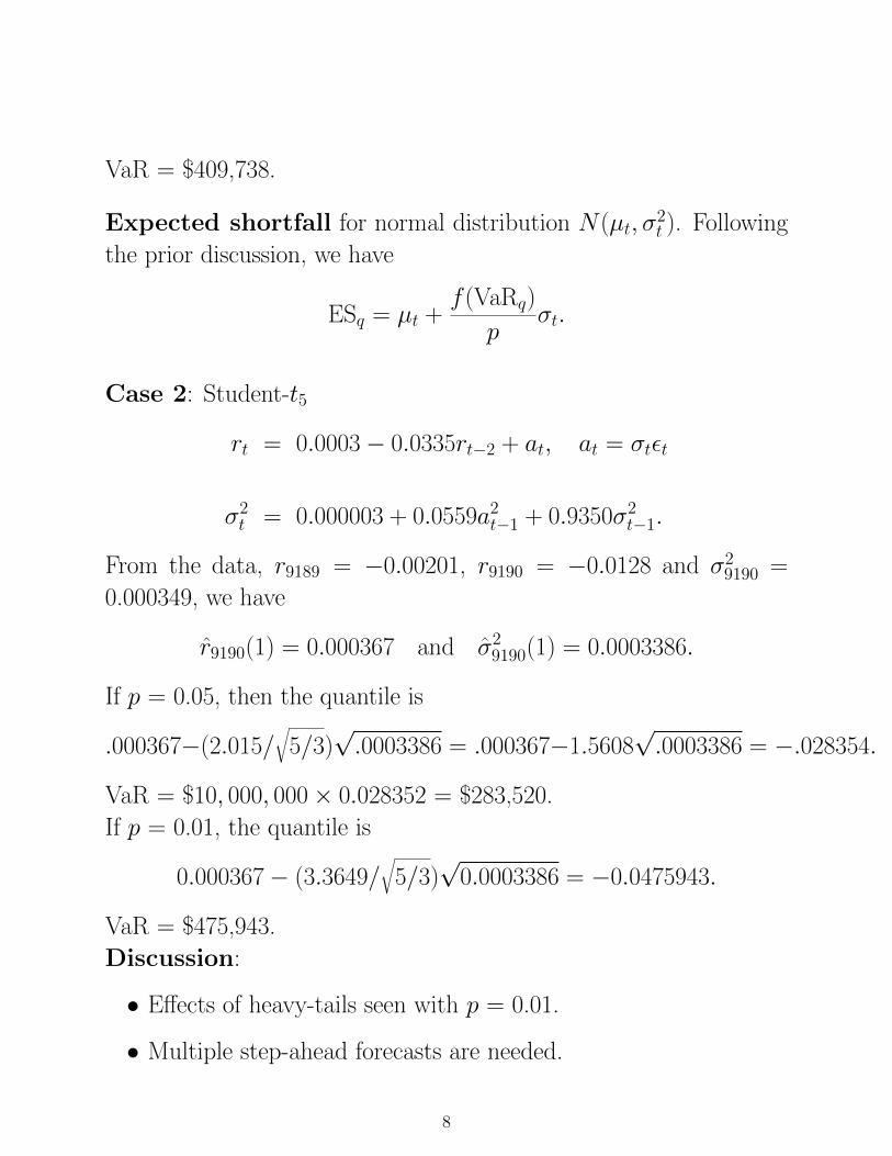
VaR = $409,738.

Expected shortfall for normal distribution N(µt, σ2t ). Following

the prior discussion, we have

ESq = µt +f (VaRq)

pσt.

Case 2: Student-t5

rt = 0.0003− 0.0335rt−2 + at, at = σtεt

σ2t = 0.000003 + 0.0559a2t−1 + 0.9350σ2t−1.

From the data, r9189 = −0.00201, r9190 = −0.0128 and σ29190 =

0.000349, we have

r9190(1) = 0.000367 and σ29190(1) = 0.0003386.

If p = 0.05, then the quantile is

.000367−(2.015/√

5/3)√.0003386 = .000367−1.5608

√.0003386 = −.028354.

VaR = $10, 000, 000× 0.028352 = $283,520.

If p = 0.01, the quantile is

0.000367− (3.3649/√

5/3)√

0.0003386 = −0.0475943.

VaR = $475,943.

Discussion:

• Effects of heavy-tails seen with p = 0.01.

• Multiple step-ahead forecasts are needed.

8

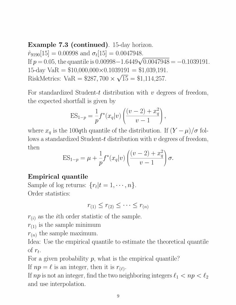
Example 7.3 (continued). 15-day horizon.

r9190[15] = 0.00998 and σt[15] = 0.0047948.

If p= 0.05, the quantile is 0.00998−1.6449√

0.0047948 =−0.1039191.

15-day VaR = $10,000,000×0.1039191 = $1,039,191.

RiskMetrics: VaR = $287, 700×√

15 = $1,114,257.

For standardized Student-t distribution with v degrees of freedom,

the expected shortfall is given by

ES1−p =1

pf ∗(xq|v)

(v − 2) + x2qv − 1

,where xq is the 100qth quantile of the distribution. If (Y −µ)/σ fol-

lows a standardized Student-t distribution with v degrees of freedom,

then

ES1−p = µ +1

pf ∗(xq|v)

(v − 2) + x2qv − 1

σ.

Empirical quantile

Sample of log returns: {rt|t = 1, · · · , n}.Order statistics:

r(1) ≤ r(2) ≤ · · · ≤ r(n)

r(i) as the ith order statistic of the sample.

r(1) is the sample minimum

r(n) the sample maximum.

Idea: Use the empirical quantile to estimate the theoretical quantile

of rt.

For a given probability p, what is the empirical quantile?

If np = ` is an integer, then it is r(`).

If np is not an integer, find the two neighboring integers `1 < np < `2and use interpolation.

9

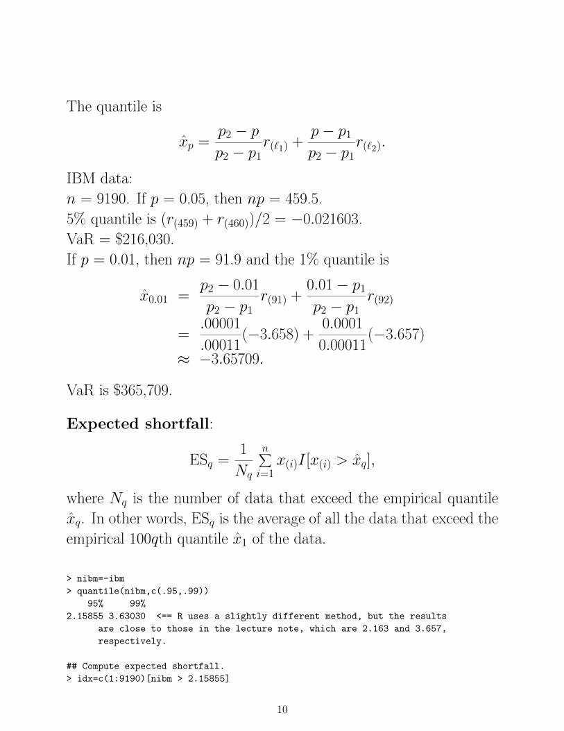
The quantile is

xp =p2 − pp2 − p1

r(`1) +p− p1p2 − p1

r(`2).

IBM data:

n = 9190. If p = 0.05, then np = 459.5.

5% quantile is (r(459) + r(460))/2 = −0.021603.

VaR = $216,030.

If p = 0.01, then np = 91.9 and the 1% quantile is

x0.01 =p2 − 0.01

p2 − p1r(91) +

0.01− p1p2 − p1

r(92)

=.00001

.00011(−3.658) +

0.0001

0.00011(−3.657)

≈ −3.65709.

VaR is $365,709.

Expected shortfall:

ESq =1

Nq

n∑i=1x(i)I [x(i) > xq],

where Nq is the number of data that exceed the empirical quantile

xq. In other words, ESq is the average of all the data that exceed the

empirical 100qth quantile x1 of the data.

> nibm=-ibm

> quantile(nibm,c(.95,.99))

95% 99%

2.15855 3.63030 <== R uses a slightly different method, but the results

are close to those in the lecture note, which are 2.163 and 3.657,

respectively.

## Compute expected shortfall.

> idx=c(1:9190)[nibm > 2.15855]

10

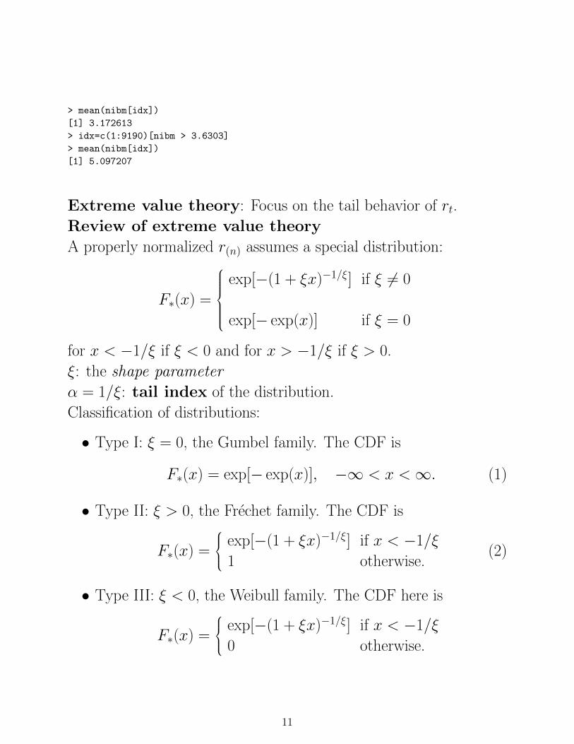
> mean(nibm[idx])

[1] 3.172613

> idx=c(1:9190)[nibm > 3.6303]

> mean(nibm[idx])

[1] 5.097207

Extreme value theory: Focus on the tail behavior of rt.

Review of extreme value theory

A properly normalized r(n) assumes a special distribution:

F∗(x) =

exp[−(1 + ξx)−1/ξ] if ξ 6= 0

exp[− exp(x)] if ξ = 0

for x < −1/ξ if ξ < 0 and for x > −1/ξ if ξ > 0.

ξ: the shape parameter

α = 1/ξ: tail index of the distribution.

Classification of distributions:

• Type I: ξ = 0, the Gumbel family. The CDF is

F∗(x) = exp[− exp(x)], −∞ < x <∞. (1)

• Type II: ξ > 0, the Frechet family. The CDF is

F∗(x) =

exp[−(1 + ξx)−1/ξ] if x < −1/ξ

1 otherwise.(2)

• Type III: ξ < 0, the Weibull family. The CDF here is

F∗(x) =

exp[−(1 + ξx)−1/ξ] if x < −1/ξ

0 otherwise.

11

The probability density function (pdf) of the normalized minimum

is

f∗(x) =

(1 + ξx)−1/ξ−1 exp[−(1 + ξx)−1/ξ] if ξ 6= 0

exp[x− exp(x)] if ξ = 0

where −∞ < x <∞ for ξ = 0, x < −1/ξ for ξ < 0 and x > −1/ξ

for ξ > 0.

How to use the EVT distribution?

If we know the three parameters, we can compute the quantile!

Empirical estimation

Divide the sample into non-overlapping subsamples.

Suppose there are T data points, we devide the data as

{r1, · · · , rn|rn+1, · · · , r2n|r2n+1, · · · , r3n| · · · |r(g−1)n+1, · · · , rng},

n: size of subgroup

Idea: find the minimum of each subgroup. These minima are the

data used to estimate the three parameters.

Several estimation methods available. We use maximum likelihood

estimates.

IBM data:

12

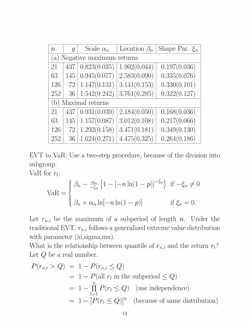
n g Scale αn Location βn Shape Par. ξn(a) Negative maximum returns

21 437 0.823(0.035) 1.902(0.044) 0.197(0.036)

63 145 0.945(0.077) 2.583(0.090) 0.335(0.076)

126 72 1.147(0.131) 3.141(0.153) 0.330(0.101)

252 36 1.542(0.242) 3.761(0.285) 0.322(0.127)

(b) Maximal returns

21 437 0.931(0.039) 2.184(0.050) 0.168(0.036)

63 145 1.157(0.087) 3.012(0.108) 0.217(0.066)

126 72 1.292(0.158) 3.471(0.181) 0.349(0.130)

252 36 1.624(0.271) 4.475(0.325) 0.264(0.186)

EVT to VaR: Use a two-step procedure, because of the division into

subgroup.

VaR for rt:

VaR =

βn − αn

−ξn

{1− [−n ln(1− p)]−ξn

}if −ξn 6= 0

βn + αn ln[−n ln(1− p)] if ξn = 0.

Let rn,i be the maximum of a subperiod of length n. Under the

traditional EVT, rn,i follows a generalized extreme value distribution

with parameter (xi,sigma,mu).

What is the relationship between quantile of rn,i and the return rt?

Let Q be a real number.

P (rn,i > Q) = 1− P (rn,i ≤ Q)

= 1− P (all rt in the subperiod ≤ Q)

= 1−n∏t=1

P (rt ≤ Q) (use independence)

= 1− [P (rt ≤ Q)]n (because of same distribution)

13

Consequently, let p be a small upper tail probability of rt and Q be

the corresponding quantile. That is,

P (rt ≤ Q) = 1− p

From the above equation, we have

P (rn,i > Q) = 1− (1− p)n.

Therefore,

P (rn,i ≤ Q) = 1− P (rn,i > Q) = (1− p)n.

This means that Q is the (1 − p)n-th quantile of the generalized

extreme value distribution.

Takeaway: For a small probability p, compute (1 − p)n, where n

is the length of subperiod, then VaR can be obtained by finding the

(1− p)n-th quantile of the extreme value distribution.

For IBM data, if n = 63 (quarterly minima), then αn = 0.945,

βn = −2.583, and ξn = 0.335. If p = 0.01, the VaR is

VaR = 2.583− 0.945

−0.335

{1− [−63 ln(1− 0.01)]−0.335

}= 3.04969

VaR is $304,969.

If p = 0.05, then VaR is $166,641.

For n = 21, the results are:

VaR = $340,013 for p = 0.01;

VaR = $184,127 for p = 0.05.

Discussion:

• Results depend on the choice of n

14

• VaR seems low, but it might be due to the choice of p.

If p = 0.001, then

VaR = $546,641 for the Gaussian AR(2)-GARCH(1,1) model

VaR = $666,590 for the extreme value theory with n = 21.

Additional information on applying extreme value theory to value at

risk calculation.

To traditional approach of EVT

Return Level: It is a risk measure based on the idea of subperiods.

The g n-subperiod return level, Ln,g, is the level that is exceeded in

one out of every g subperiods of length n.

P (rn,i < Ln,g) =1

g,

where n is the length of subperiod used in estimating the GEV model

and rn,i denotes subperiod minimum. For sufficiently large n,

Ln,g = βn +αn−ξn{[− ln(1− 1/g)]−ξn − 1},

where the shape parameter ξn 6= 0.

For a short position, the return level is

Ln,g = βn +αn−ξn{1− [− ln(1− 1/g)]−1/ξn}.

Summary of IBM data:

Position = $10 million.

If p = 0.05, then

1. $308,200 for the RiskMetrics,

2. $287,200 for an AR(2)-GARCH(1,1) model,

15

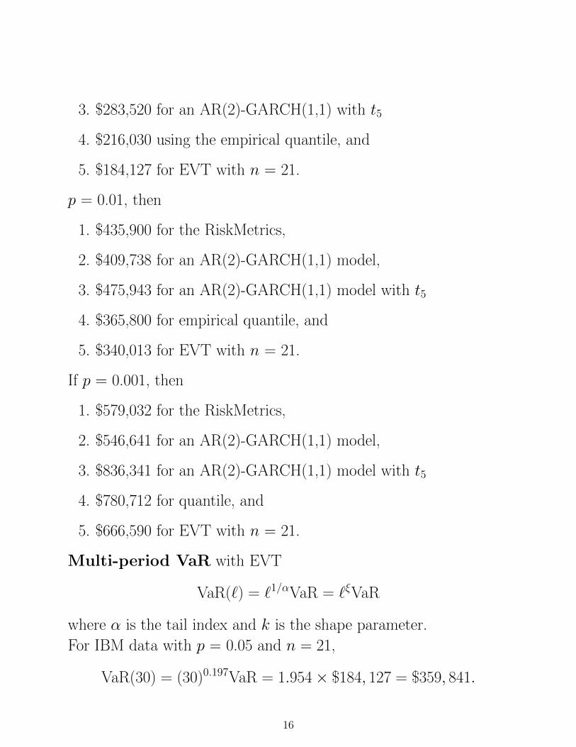
3. $283,520 for an AR(2)-GARCH(1,1) with t5

4. $216,030 using the empirical quantile, and

5. $184,127 for EVT with n = 21.

p = 0.01, then



3. $475,943 for an AR(2)-GARCH(1,1) model with t5

4. $365,800 for empirical quantile, and

5. $340,013 for EVT with n = 21.

If p = 0.001, then



3. $836,341 for an AR(2)-GARCH(1,1) model with t5

4. $780,712 for quantile, and

5. $666,590 for EVT with n = 21.

Multi-period VaR with EVT

VaR(`) = `1/αVaR = `ξVaR

where α is the tail index and k is the shape parameter.

For IBM data with p = 0.05 and n = 21,

VaR(30) = (30)0.197VaR = 1.954× $184, 127 = $359, 841.

16

New approach to VaR

Based on Exceedances over a high threshold

Idea: frequency of big returns and their magnitudes are important.

Statistical theory:

Two-dimensional Poisson process

Two possible cases:

Homogeneous: parameters are fixed over time

Non-homogeneous case: parameters are time-varying, according to

some explanatory variables.

IBM data: homogeneous model

Thr. Exc. Shape Par. ξ Log(Scale) ln(α) Location β

(a) Original log returns

3.0% 175 0.30697(0.09015) 0.30699(0.12380) 4.69204(0.19058)

2.5% 310 0.26418(0.06501) 0.31529(0.11277) 4.74062(0.18041)

2.0% 554 0.18751(0.04394) 0.27655(0.09867) 4.81003(0.17209)

(b) Removing the sample mean

3.0% 184 0.30516(0.08824) 0.30807(0.12395) 4.73804(0.19151)

2.5% 334 0.28179(0.06737) 0.31968(0.12065) 4.76808(0.18533)

2.0% 590 0.19260(0.04357) 0.27917(0.09913) 4.84859(0.17255)

VaR calculation:

VaR =

β + α

−ξ

{1− [−T ln(1− p)]−ξ

}if −ξ 6= 0

β + α ln[−T ln(1− p)] if ξ = 0

where T = 252, the number trading days in a year.

IBM data: VaR of 5% & 1%

• Case I: original returns

17

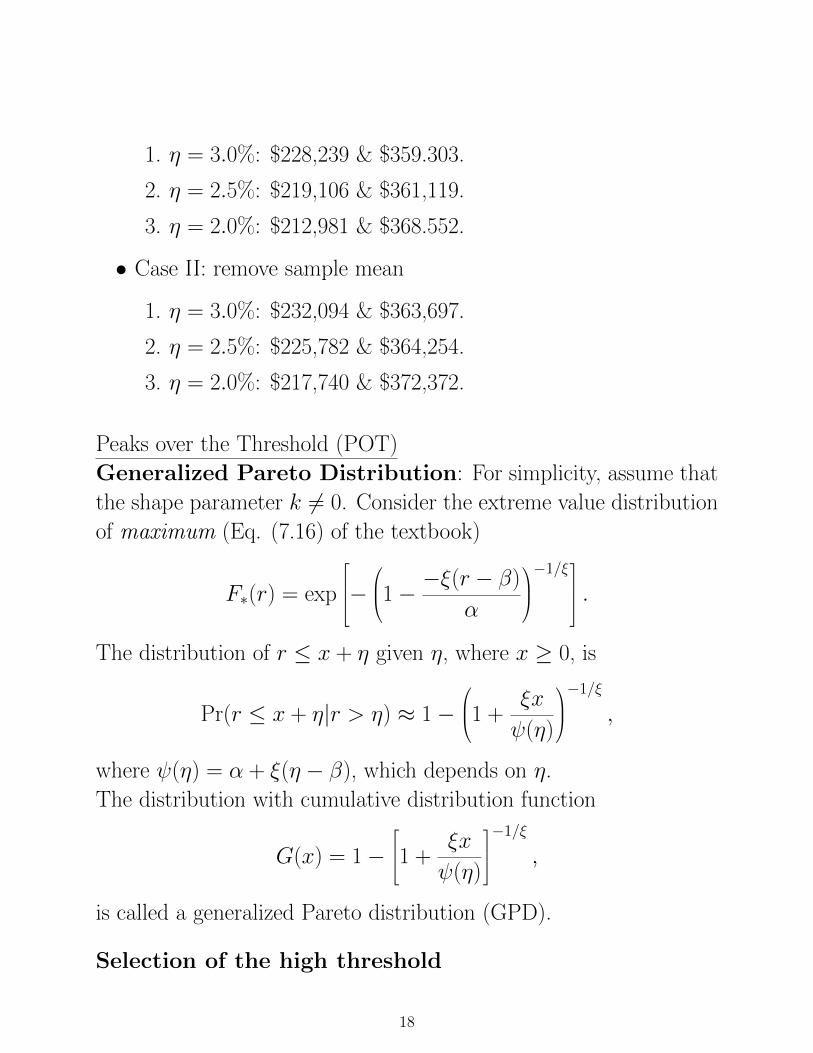
1. η = 3.0%: $228,239 & $359.303.

2. η = 2.5%: $219,106 & $361,119.

3. η = 2.0%: $212,981 & $368.552.

• Case II: remove sample mean

1. η = 3.0%: $232,094 & $363,697.

2. η = 2.5%: $225,782 & $364,254.

3. η = 2.0%: $217,740 & $372,372.

Peaks over the Threshold (POT)

Generalized Pareto Distribution: For simplicity, assume that

the shape parameter k 6= 0. Consider the extreme value distribution

of maximum (Eq. (7.16) of the textbook)

F∗(r) = exp

−1− −ξ(r − β)

α

−1/ξ .

The distribution of r ≤ x + η given η, where x ≥ 0, is

Pr(r ≤ x + η|r > η) ≈ 1−1 +

ξx

ψ(η)

−1/ξ

,

where ψ(η) = α + ξ(η − β), which depends on η.

The distribution with cumulative distribution function

G(x) = 1−1 +

ξx

ψ(η)

−1/ξ

,

is called a generalized Pareto distribution (GPD).

Selection of the high threshold

18

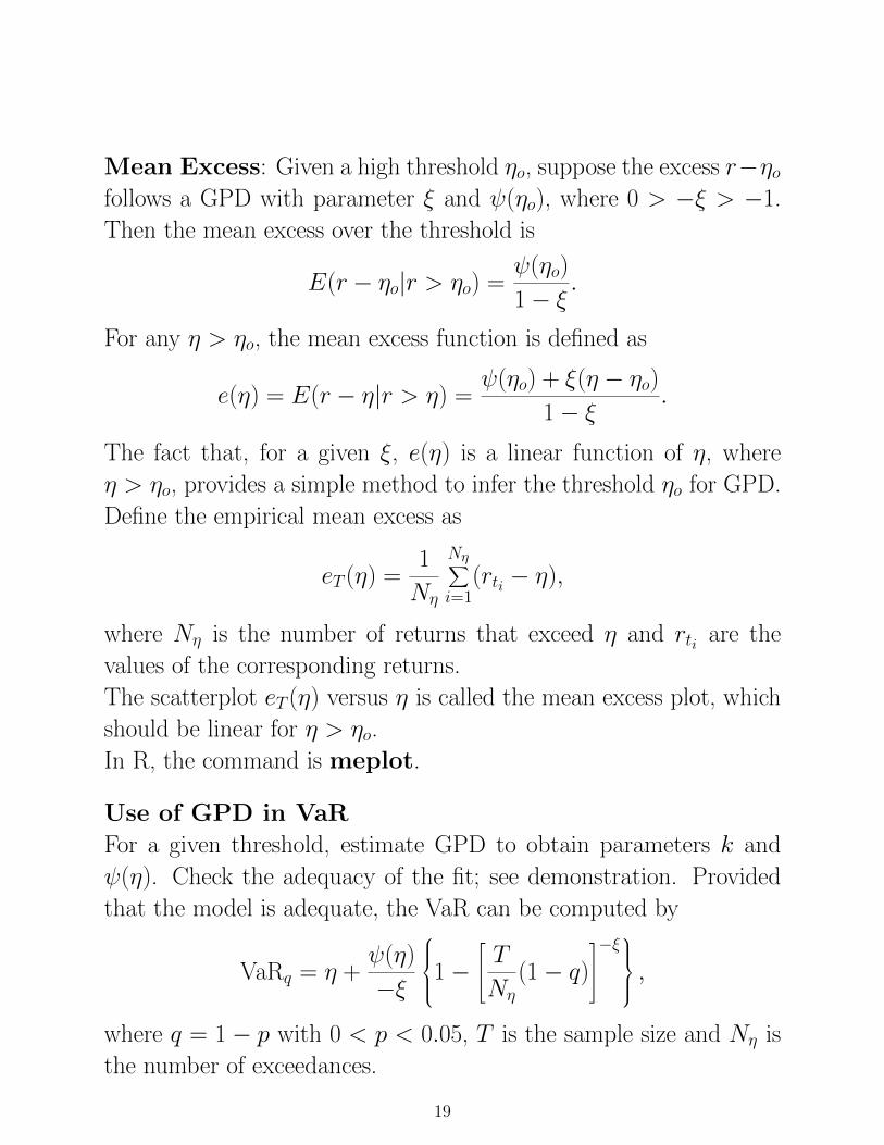
Mean Excess: Given a high threshold ηo, suppose the excess r−ηofollows a GPD with parameter ξ and ψ(ηo), where 0 > −ξ > −1.

Then the mean excess over the threshold is

E(r − ηo|r > ηo) =ψ(ηo)

1− ξ.

For any η > ηo, the mean excess function is defined as

e(η) = E(r − η|r > η) =ψ(ηo) + ξ(η − ηo)

1− ξ.

The fact that, for a given ξ, e(η) is a linear function of η, where

η > ηo, provides a simple method to infer the threshold ηo for GPD.

Define the empirical mean excess as

eT (η) =1

Nη

Nη∑i=1

(rti − η),

where Nη is the number of returns that exceed η and rti are the

values of the corresponding returns.

The scatterplot eT (η) versus η is called the mean excess plot, which

should be linear for η > ηo.

In R, the command is meplot.

Use of GPD in VaR

For a given threshold, estimate GPD to obtain parameters k and

ψ(η). Check the adequacy of the fit; see demonstration. Provided

that the model is adequate, the VaR can be computed by

VaRq = η +ψ(η)

−ξ

1− TNη

(1− q)−ξ ,

where q = 1− p with 0 < p < 0.05, T is the sample size and Nη is

the number of exceedances.

19

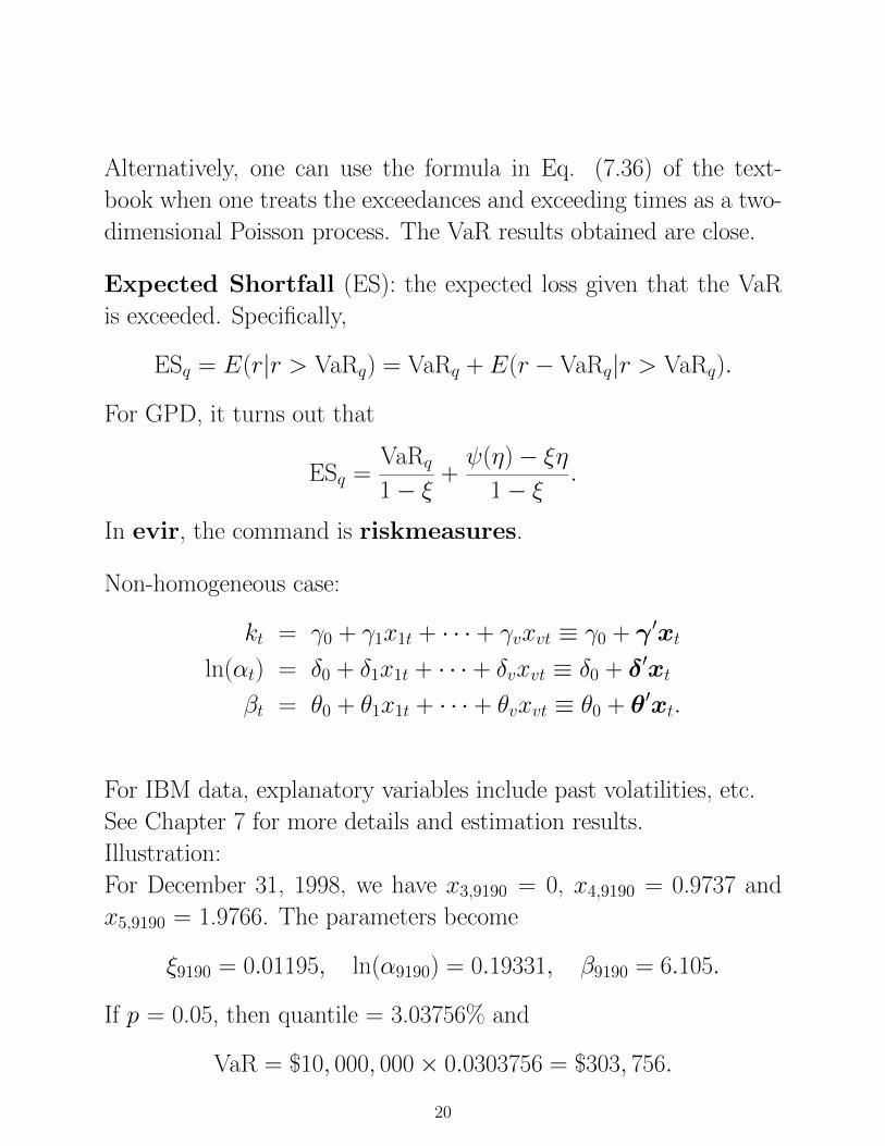
Alternatively, one can use the formula in Eq. (7.36) of the text-

book when one treats the exceedances and exceeding times as a two-

dimensional Poisson process. The VaR results obtained are close.

Expected Shortfall (ES): the expected loss given that the VaR

is exceeded. Specifically,

ESq = E(r|r > VaRq) = VaRq + E(r − VaRq|r > VaRq).

For GPD, it turns out that

ESq =VaRq

1− ξ+ψ(η)− ξη

1− ξ.

In evir, the command is riskmeasures.

Non-homogeneous case:

kt = γ0 + γ1x1t + · · · + γvxvt ≡ γ0 + γ ′xt

ln(αt) = δ0 + δ1x1t + · · · + δvxvt ≡ δ0 + δ′xt

βt = θ0 + θ1x1t + · · · + θvxvt ≡ θ0 + θ′xt.

For IBM data, explanatory variables include past volatilities, etc.

See Chapter 7 for more details and estimation results.

Illustration:

For December 31, 1998, we have x3,9190 = 0, x4,9190 = 0.9737 and

x5,9190 = 1.9766. The parameters become

ξ9190 = 0.01195, ln(α9190) = 0.19331, β9190 = 6.105.

If p = 0.05, then quantile = 3.03756% and

VaR = $10, 000, 000× 0.0303756 = $303, 756.

20

If p = 0.01, then Var is $497,425.

For December 30, 1998, we have x3,9189 = 1, x4,9189 = 0.9737 and

x5,9189 = 1.8757 and

ξ9189 = 0.2500, ln(α9189) = 0.52385, β9189 = 5.8834.

The 5% VaR becomes

VaR = $10, 000, 000× 0.0269139 = $269, 139.

If p = 0.01, then VaR becomes $448,323.

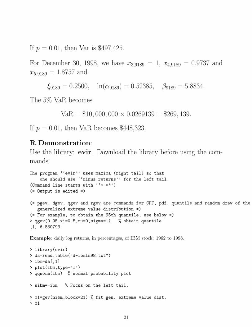
R Demonstration:

Use the library: evir. Download the library before using the com-

mands.

The program ‘‘evir’’ uses maxima (right tail) so that

one should use ‘‘minus returns’’ for the left tail.

(Command line starts with ‘‘> *’’)

(* Output is edited *)

(* pgev, dgev, qgev and rgev are commands for CDF, pdf, quantile and random draw of the

generalized extreme value distribution *)

(* For example, to obtain the 95th quantile, use below *)

> qgev(0.95,xi=0.5,mu=0,sigma=1) % obtain quantile

[1] 6.830793

Example: daily log returns, in percentages, of IBM stock: 1962 to 1998.

> library(evir)

> da=read.table("d-ibmln98.txt")

> ibm=da[,1]

> plot(ibm,type=’l’)

> qqnorm(ibm) % normal probability plot

> nibm=-ibm % Focus on the left tail.

> m1=gev(nibm,block=21) % fit gen. extreme value dist.

> m1

21

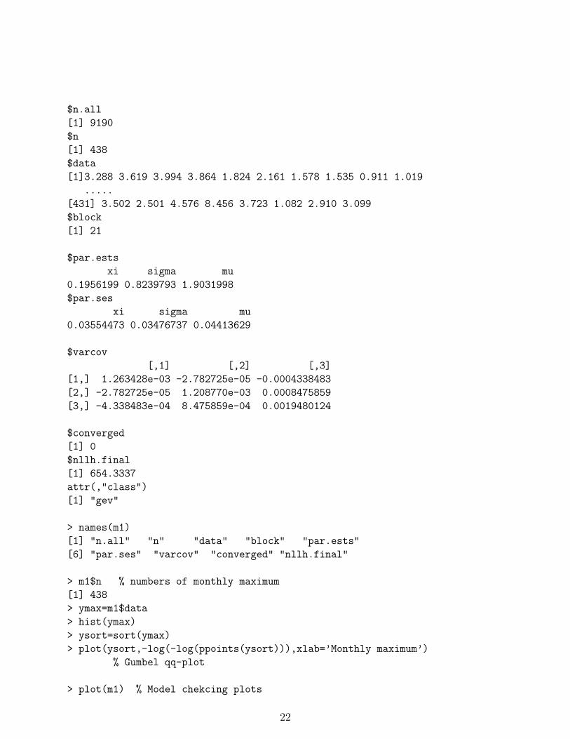
$n.all

[1] 9190

$n

[1] 438

$data

[1]3.288 3.619 3.994 3.864 1.824 2.161 1.578 1.535 0.911 1.019

.....

[431] 3.502 2.501 4.576 8.456 3.723 1.082 2.910 3.099

$block

[1] 21

$par.ests

xi sigma mu

0.1956199 0.8239793 1.9031998

$par.ses

xi sigma mu

0.03554473 0.03476737 0.04413629

$varcov

[,1] [,2] [,3]

[1,] 1.263428e-03 -2.782725e-05 -0.0004338483

[2,] -2.782725e-05 1.208770e-03 0.0008475859

[3,] -4.338483e-04 8.475859e-04 0.0019480124

$converged

[1] 0

$nllh.final

[1] 654.3337

attr(,"class")

[1] "gev"

> names(m1)

[1] "n.all" "n" "data" "block" "par.ests"

[6] "par.ses" "varcov" "converged" "nllh.final"

> m1$n % numbers of monthly maximum

[1] 438

> ymax=m1$data

> hist(ymax)

> ysort=sort(ymax)

> plot(ysort,-log(-log(ppoints(ysort))),xlab=’Monthly maximum’)

% Gumbel qq-plot

> plot(m1) % Model chekcing plots

22

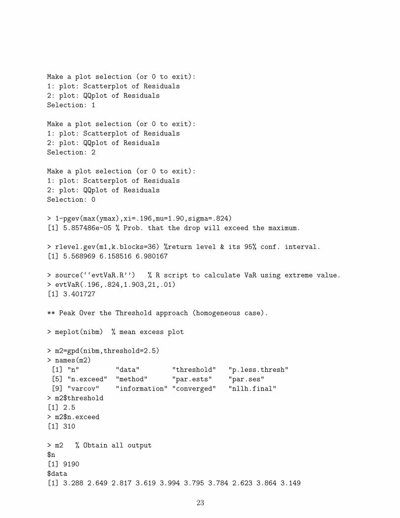
Make a plot selection (or 0 to exit):

1: plot: Scatterplot of Residuals

2: plot: QQplot of Residuals

Selection: 1




Selection: 2




Selection: 0

> 1-pgev(max(ymax),xi=.196,mu=1.90,sigma=.824)

[1] 5.857486e-05 % Prob. that the drop will exceed the maximum.

> rlevel.gev(m1,k.blocks=36) %return level & its 95% conf. interval.

[1] 5.568969 6.158516 6.980167

> source(‘‘evtVaR.R’’) % R script to calculate VaR using extreme value.

> evtVaR(.196,.824,1.903,21,.01)

[1] 3.401727

** Peak Over the Threshold approach (homogeneous case).

> meplot(nibm) % mean excess plot

> m2=gpd(nibm,threshold=2.5)

> names(m2)

[1] "n" "data" "threshold" "p.less.thresh"

[5] "n.exceed" "method" "par.ests" "par.ses"

[9] "varcov" "information" "converged" "nllh.final"

> m2$threshold

[1] 2.5

> m2$n.exceed

[1] 310

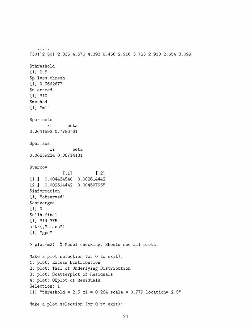
> m2 % Obtain all output

$n

[1] 9190

$data

[1] 3.288 2.649 2.817 3.619 3.994 3.795 3.784 2.623 3.864 3.149

23

.....

[301]2.501 2.835 4.576 4.393 8.456 2.916 3.723 2.910 2.654 3.099

$threshold

[1] 2.5

$p.less.thresh

[1] 0.9662677

$n.exceed

[1] 310

$method

[1] "ml"

$par.ests

xi beta

0.2641593 0.7786761

$par.ses

xi beta

0.06659234 0.06714131

$varcov

[,1] [,2]

[1,] 0.004434540 -0.002614442

[2,] -0.002614442 0.004507955

$information

[1] "observed"

$converged

[1] 0

$nllh.final

[1] 314.375

attr(,"class")

[1] "gpd"

> plot(m2) % Model checking. Should see all plots.


1: plot: Excess Distribution

2: plot: Tail of Underlying Distribution



Selection: 1

[1] "threshold = 2.5 xi = 0.264 scale = 0.779 location= 2.5"


24

1: plot: Excess Distribution

2: plot: Tail of Underlying Distribution



Selection: 0

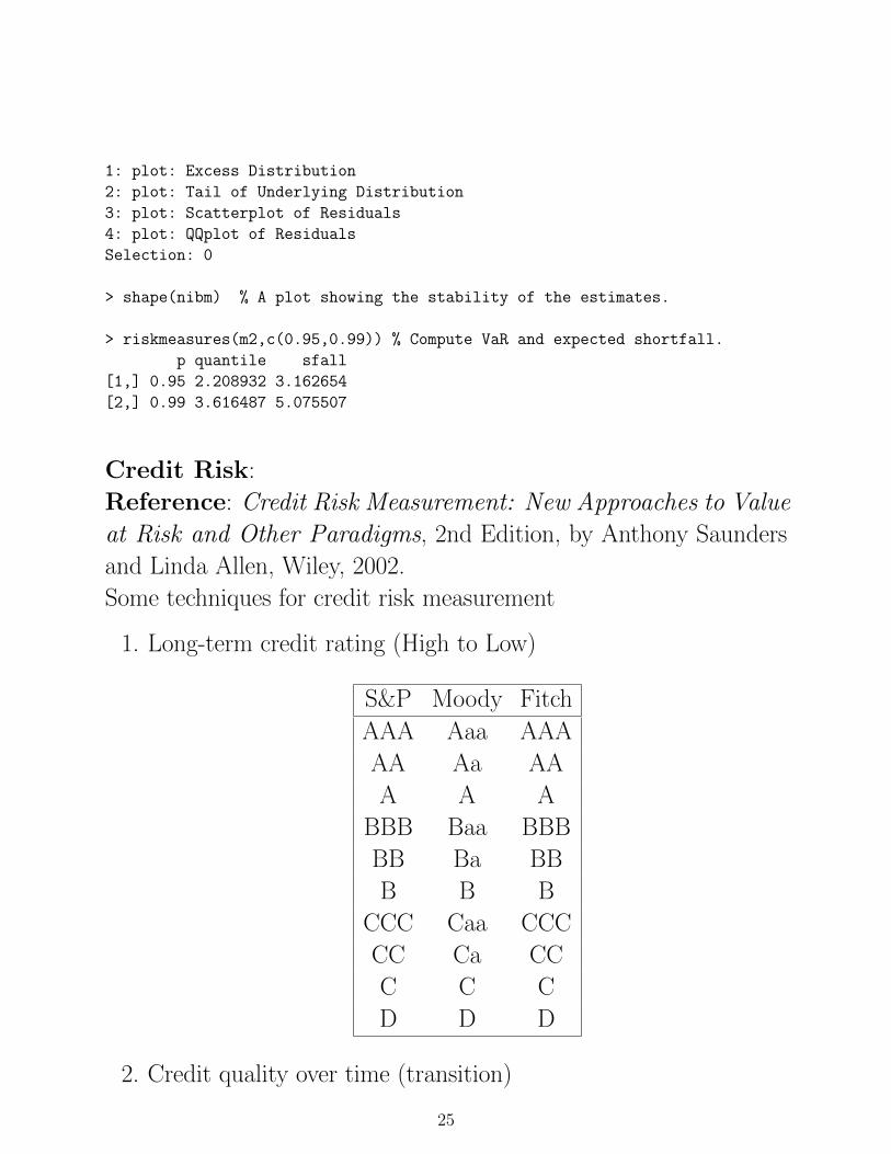
> shape(nibm) % A plot showing the stability of the estimates.

> riskmeasures(m2,c(0.95,0.99)) % Compute VaR and expected shortfall.

p quantile sfall

[1,] 0.95 2.208932 3.162654

[2,] 0.99 3.616487 5.075507

Credit Risk:

Reference: Credit Risk Measurement: New Approaches to Value

at Risk and Other Paradigms, 2nd Edition, by Anthony Saunders

and Linda Allen, Wiley, 2002.

Some techniques for credit risk measurement

1. Long-term credit rating (High to Low)

S&P Moody Fitch

AAA Aaa AAA

AA Aa AA

A A A

BBB Baa BBB

BB Ba BB

B B B

CCC Caa CCC

CC Ca CC

C C C

D D D

2. Credit quality over time (transition)

25

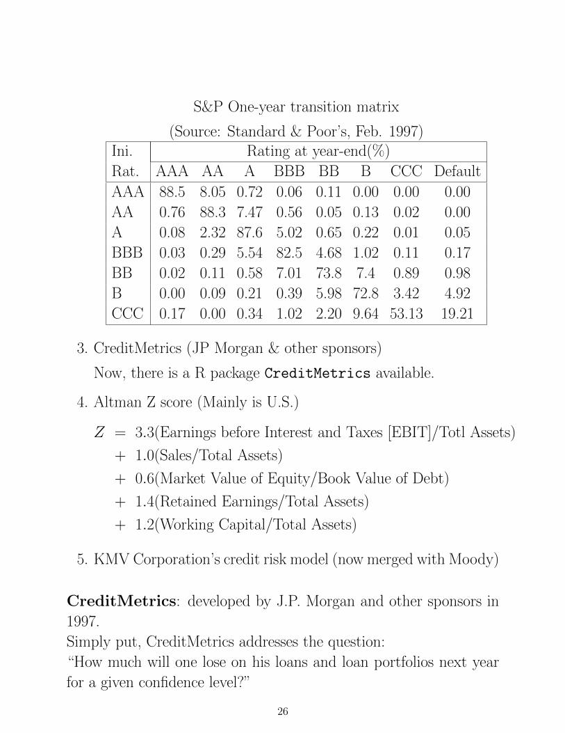
S&P One-year transition matrix

(Source: Standard & Poor’s, Feb. 1997)Ini. Rating at year-end(%)

Rat. AAA AA A BBB BB B CCC Default

AAA 88.5 8.05 0.72 0.06 0.11 0.00 0.00 0.00

AA 0.76 88.3 7.47 0.56 0.05 0.13 0.02 0.00

A 0.08 2.32 87.6 5.02 0.65 0.22 0.01 0.05

BBB 0.03 0.29 5.54 82.5 4.68 1.02 0.11 0.17

BB 0.02 0.11 0.58 7.01 73.8 7.4 0.89 0.98

B 0.00 0.09 0.21 0.39 5.98 72.8 3.42 4.92

CCC 0.17 0.00 0.34 1.02 2.20 9.64 53.13 19.21

3. CreditMetrics (JP Morgan & other sponsors)

Now, there is a R package CreditMetrics available.

4. Altman Z score (Mainly is U.S.)

Z = 3.3(Earnings before Interest and Taxes [EBIT]/Totl Assets)

+ 1.0(Sales/Total Assets)

+ 0.6(Market Value of Equity/Book Value of Debt)

+ 1.4(Retained Earnings/Total Assets)

+ 1.2(Working Capital/Total Assets)

5. KMV Corporation’s credit risk model (now merged with Moody)

CreditMetrics: developed by J.P. Morgan and other sponsors in

1997.

Simply put, CreditMetrics addresses the question:

“How much will one lose on his loans and loan portfolios next year

for a given confidence level?”

26

From the assessment of market risk, the current market value and

its volatility of a financial position play an imporant role in VaR

calculation. Application of VaR methodology to nontrabable loans

encounters some immediate problems:

1. The current market value of the loan is not directly observable,

because most loans are not traded.

2. No time-series data available to estimate the volatility.

To overcome the difficulties, we make use of

1. Available data on a borrower’s credit rating

2. The probability that the rating will change over the next year

(the rating transition matrix)

3. Recovery rates on deafulted loans

4. Credit spreads and yields in the bond (or loan) market.

Example: Consider a five-year fixed-rate loan of $100 million made

at 6% annual interest, and the borrower is rated BBB.

Note: The numerical numbers used in this example are from Chap-

ter 6 of the reference book cited above.

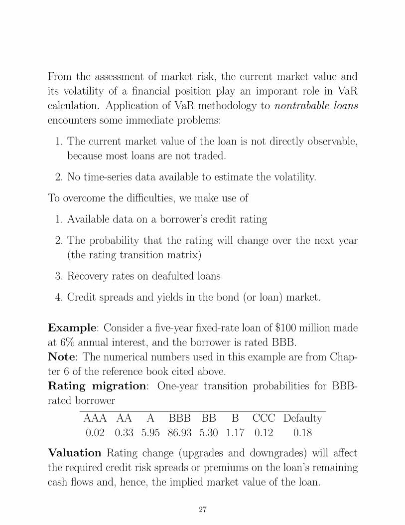
Rating migration: One-year transition probabilities for BBB-

rated borrower

AAA AA A BBB BB B CCC Defaulty

0.02 0.33 5.95 86.93 5.30 1.17 0.12 0.18

Valuation Rating change (upgrades and downgrades) will affect

the required credit risk spreads or premiums on the loan’s remaining

cash flows and, hence, the implied market value of the loan.

27

Downgrade → credit spread premium rises → present value of the

loan should fall.

Upgrade has the opposite effect.

return to the example. (after one-year and a credit rating change)

P = 6+6

1 + r1,1 + s1+

6

(1 + r1,2 + s2)2+

6

(1 + r1,3 + s3)3+

106

(1 + r1,4 + s4)4,

where r1,i are the risk-free rates on zero-coupon U.S. Treasury bonds

expected to exist one year into the future and si is the annual credit

spread on loans of a particular rating class of 1-year, 2-year, 3-year

and 4-year maturities (derived from observed spreads in the corporate

bond market over Treasuries).

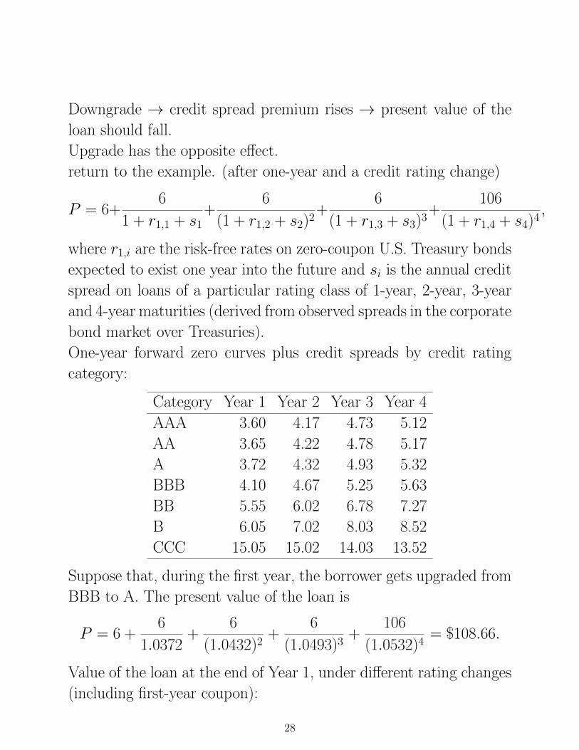
One-year forward zero curves plus credit spreads by credit rating

category:

Category Year 1 Year 2 Year 3 Year 4

AAA 3.60 4.17 4.73 5.12

AA 3.65 4.22 4.78 5.17

A 3.72 4.32 4.93 5.32

BBB 4.10 4.67 5.25 5.63

BB 5.55 6.02 6.78 7.27

B 6.05 7.02 8.03 8.52

CCC 15.05 15.02 14.03 13.52

Suppose that, during the first year, the borrower gets upgraded from

BBB to A. The present value of the loan is

P = 6 +6

1.0372+

6

(1.0432)2+

6

(1.0493)3+

106

(1.0532)4= $108.66.

Value of the loan at the end of Year 1, under different rating changes

(including first-year coupon):

28

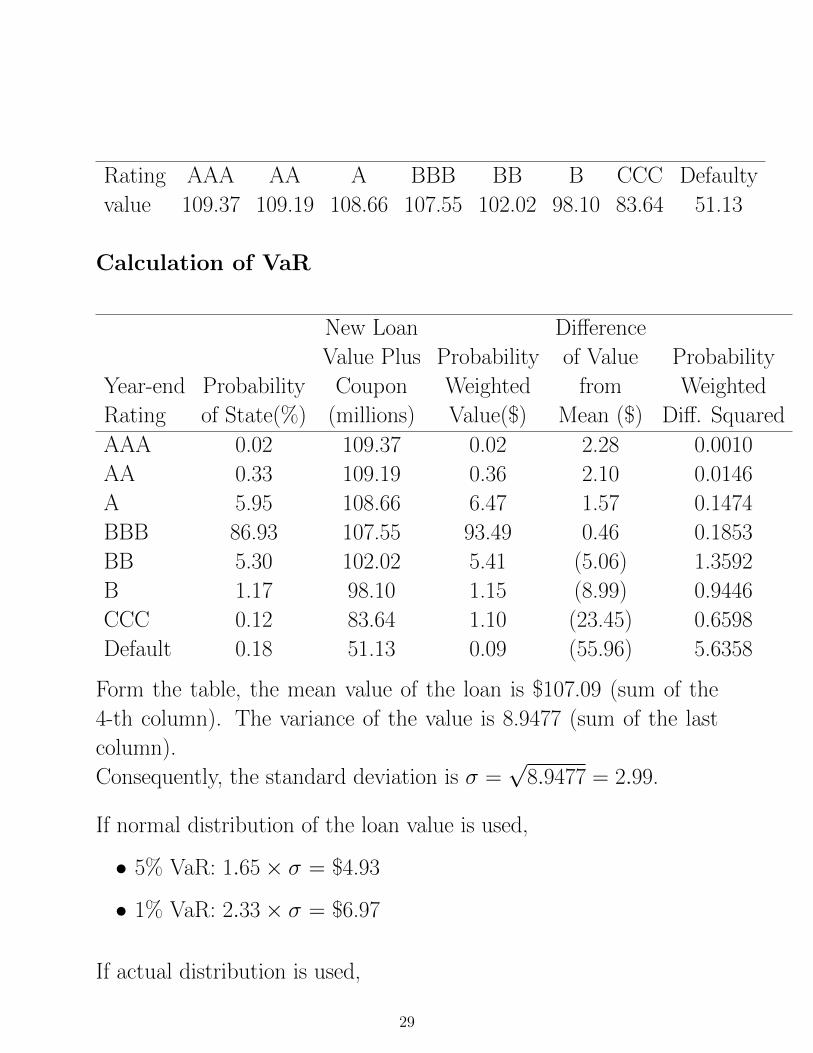
Rating AAA AA A BBB BB B CCC Defaulty

value 109.37 109.19 108.66 107.55 102.02 98.10 83.64 51.13

Calculation of VaR

New Loan Difference

Value Plus Probability of Value Probability

Year-end Probability Coupon Weighted from Weighted

Rating of State(%) (millions) Value($) Mean ($) Diff. Squared

AAA 0.02 109.37 0.02 2.28 0.0010

AA 0.33 109.19 0.36 2.10 0.0146

A 5.95 108.66 6.47 1.57 0.1474

BBB 86.93 107.55 93.49 0.46 0.1853

BB 5.30 102.02 5.41 (5.06) 1.3592

B 1.17 98.10 1.15 (8.99) 0.9446

CCC 0.12 83.64 1.10 (23.45) 0.6598

Default 0.18 51.13 0.09 (55.96) 5.6358

Form the table, the mean value of the loan is $107.09 (sum of the

4-th column). The variance of the value is 8.9477 (sum of the last

column).

Consequently, the standard deviation is σ =√

8.9477 = 2.99.

If normal distribution of the loan value is used,

• 5% VaR: 1.65× σ = $4.93

• 1% VaR: 2.33× σ = $6.97

If actual distribution is used,

29

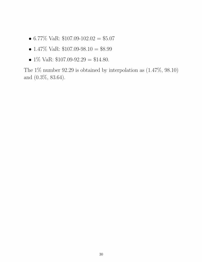
• 6.77% VaR: $107.09-102.02 = $5.07

• 1.47% VaR: $107.09-98.10 = $8.99

• 1% VaR: $107.09-92.29 = $14.80.

The 1% number 92.29 is obtained by interpolation as (1.47%, 98.10)

and (0.3%, 83.64).

30

Documents

Lecture Note of Bus 41202, Spring 2012: Value at Risk ...faculty.chicagobooth.edu/ruey.tsay/teaching/bs41202/sp2012/lec9-12.pdf · Lecture Note of Bus 41202, Spring 2012: Value at