LECTURE NOTE 1

MCE 521: Computational Fluid Dynamics

ENGR. ALIYU, S. J.

MCE 521

Advanced Computational Dynamics Modelling engineering systems using ordinary and partial differential equations; finite difference

schemes; and weighted residual methods and spectral methods. All necessary theories in order

for students to be able to use commercial computational fluid dynamics (CFD) software

proficiently.

1 Introduction 1

Importance of Fluids

Fluids in the pure sciences

Fluids in technology

The Study of Fluids

The theoretical approach

Experimental fluid dynamics

Computational fluid dynamics

Introduction

It takes little more than a brief look around for us to recognize that fluid dynamics is one of the

most important of all areas of physics—life as we know it would not exist without fluids, and

without the behavior that fluids exhibit. The air we breathe and the water we drink (and which

makes up most of our body mass) are fluids. Motion of air keeps us comfortable in a warm room,

and air provides the oxygen we need to sustain life. Similarly, most of our (liquid) body fluids

are water based. And proper motion of these fluids within our bodies, even down to the cellular

level, is essential to good health. It is clear that fluids are completely necessary for the support of

carbon-based life forms.

But the study of biological systems is only one (and a very recent one) possible application of a

knowledge of fluid dynamics. Fluids occur, and often dominate physical phenomena, on all

macroscopic (non-quantum) length scales of the known universe—from the mega-par-secs of

galactic structure down to the micro and even nano-scales of biological cell activity. In a more

practical setting, we easily see that fluids greatly influence our comfort (or lack thereof); they are

involved in our transportation systems in many ways; they have an effect on our recreation (e.g.,

basketballs and footballs are inflated with air) and entertainment (the sound from the speakers of

a TV would not reach our ears in the absence of air), and even on our sleep (water beds!). From

this it is fairly easy to see that engineers must have at least a working knowledge of fluid

behavior to accurately analyze many, if not most, of the systems they will encounter. It is the

goal of these lecture notes to help students in this process of gaining an understanding of, and an

appreciation for, fluid motion—what can be done with it, what it might do to you, how to

analyze and predict it. In this introductory chapter we will begin by further stressing the

importance of fluid dynamics by providing specific examples from both the pure sciences and

from technology in which knowledge of this field is essential to an understanding of the physical

phenomena (and, hence, the beginnings of a predictive capability—e.g., the weather) and/or the

ability to design and control devices such as internal combustion engines. We then describe three

main approaches to the study of fluid dynamics: i) theoretical, ii) experimental and iii)

computational.

Importance of Fluids

We have already emphasized the overall importance of fluids in a general way, and here we will

augment this with a number of specific examples. We somewhat arbitrarily classify these in two

main categories:

i) Physical and natural science, and

ii) Technology. Clearly, the second of these is often of more interest to an engineering student,

but in the modern era of emphasis on interdisciplinary studies, the more scientific and

mathematical aspects of fluid phenomena are becoming increasingly important.

Fluids in the pure sciences

The following list, which is by no means all inclusive, provides some examples of fluid

phenomena often studied by physicists, astronomers, biologists and others who do not

necessarily deal in the design and analysis of devices. The accompanying figures highlight some

of these areas.

1. Atmospheric sciences

(a) Global circulation: long-range weather prediction; analysis of climate change (global

warming)

(b) Meso-scale weather patterns: short-range weather prediction; tornado and hurricane

warnings; pollutant transport

2. Oceanography

(a) Ocean circulation patterns: causes of El Ni˜no, effects of ocean currents on weather and

climate

(b) Effects of pollution on living organisms

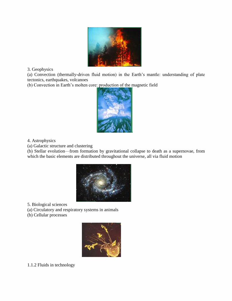
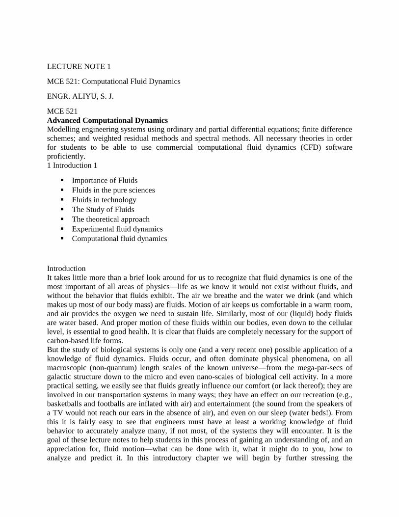
3. Geophysics

(a) Convection (thermally-driven fluid motion) in the Earth’s mantle: understanding of plate

tectonics, earthquakes, volcanoes

(b) Convection in Earth’s molten core: production of the magnetic field

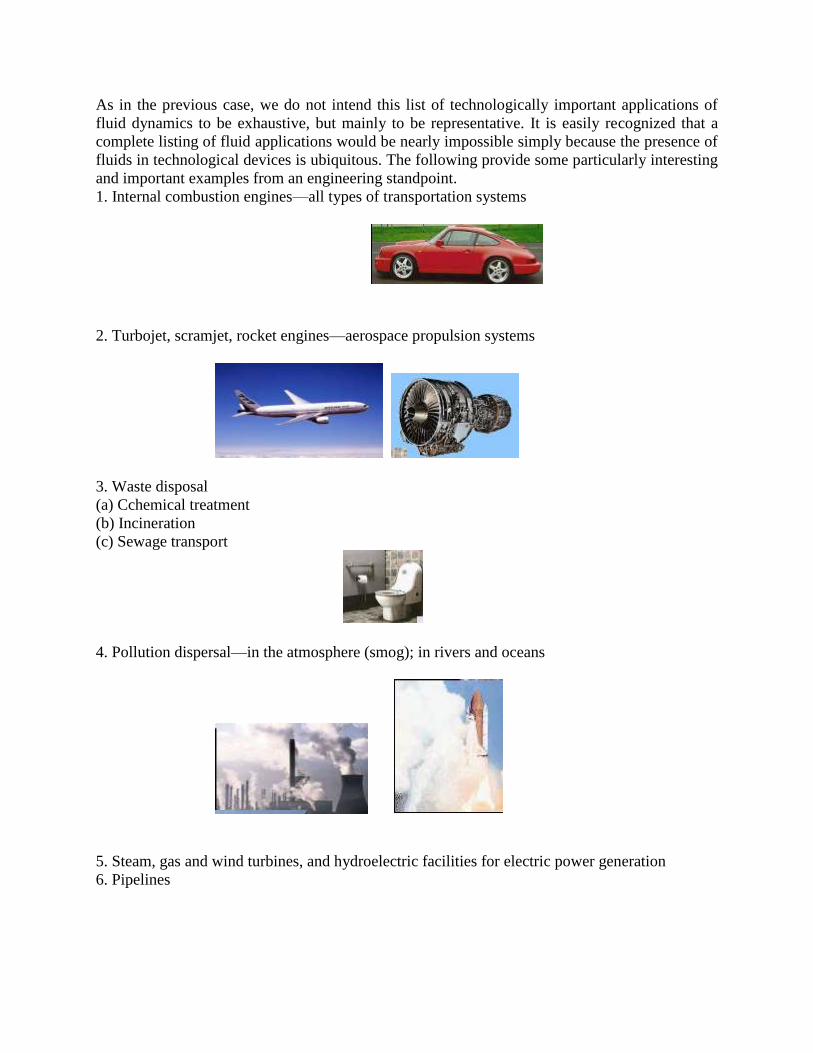
4. Astrophysics

(a) Galactic structure and clustering

(b) Stellar evolution—from formation by gravitational collapse to death as a supernovae, from

which the basic elements are distributed throughout the universe, all via fluid motion

5. Biological sciences

(a) Circulatory and respiratory systems in animals

(b) Cellular processes

1.1.2 Fluids in technology

As in the previous case, we do not intend this list of technologically important applications of

fluid dynamics to be exhaustive, but mainly to be representative. It is easily recognized that a

complete listing of fluid applications would be nearly impossible simply because the presence of

fluids in technological devices is ubiquitous. The following provide some particularly interesting

and important examples from an engineering standpoint.

1. Internal combustion engines—all types of transportation systems

2. Turbojet, scramjet, rocket engines—aerospace propulsion systems

3. Waste disposal

(a) Cchemical treatment

(b) Incineration

(c) Sewage transport

4. Pollution dispersal—in the atmosphere (smog); in rivers and oceans

5. Steam, gas and wind turbines, and hydroelectric facilities for electric power generation

6. Pipelines

(a) Crude oil and natural gas transferral

(b) Irrigation facilities

(c) Office building and household plumbing

7. Fluid/structure interaction

(a) Design of tall buildings

(b) Continental shelf oil-drilling rigs

(c) Dams, bridges, etc.

(d) Aircraft and launch vehicle airframes and control systems

8. Heating, ventilating and air-conditioning (HVAC) systems

8. Heating, ventilating and air-conditioning (HVAC) systems

9. Cooling systems for high-density electronic devices—digital computers from PCs to

supercomputers

10. Solar heat and geothermal heat utilization

11. Artificial hearts, kidney dialysis machines, insulin pumps

12. Manufacturing processes

(a) Spray painting automobiles, trucks, etc.

(b) Filling of containers, e.g., cans of soup, cartons of milk, plastic bottles of soda

(c) Operation of various hydraulic devices

(d) Chemical vapor deposition, drawing of synthetic fibers, wires, rods, etc.

We conclude from the various preceding examples that there is essentially no part of our daily

lives that is not influenced by fluids. As a consequence, it is extremely important that engineers

be capable of predicting fluid motion. In particular, the majority of engineers who are not fluid

dynamicists still will need to interact, on a technical basis, with those who are quite frequently;

and a basic competence in fluid dynamics will make such interactions more productive.

The Study of Fluids

We begin by introducing the ―intuitive notion‖ of what constitutes a fluid. As already indicated

we are accustomed to being surrounded by fluids—both gases and liquids are fluids—and we

deal with these in numerous forms on a daily basis. As a consequence, we have a fairly good

intuition regarding what is, and is not, a fluid; in short we would probably simply say that a fluid

is ―anything that flows.‖ This is actually a good practical view to take, most of the time. But we

will later see that it leaves out some things that are fluids, and includes things that are not. So if

we are to accurately analyze the behavior of fluids it will be necessary to have a more precise

definition. It is interesting to note that the formal study of fluids began at least 500 hundred years

ago with the work of Leonardo da Vinci, but obviously a basic practical understanding of the

behavior of fluids was available much earlier, at least by the time of the ancient Egyptians; in

fact, the homes of well-to-do Romans had flushing toilets not very different from those in

modern 21st-Century houses, and the Roman aquaducts are still considered a tremendous

engineering feat. Thus, already by the time of the Roman Empire enough practical information

had been accumulated to permit quite sophisticated applications of fluid dynamics. The more

modern understanding of fluid motion began several centuries ago with the work of L. Euler and

the Bernoullis (father and son), and the equation we know as Bernoulli’s equation (although this

equation was probably deduced by someone other than a Bernoulli). The equations we will

derive and study in these lectures were introduced by Navier in the 1820s, and the complete

system of equations representing essentially all fluid motions were given by Stokes in the 1840s.

These are now known as the Navier–Stokes equations, and they are of crucial importance in fluid

dynamics. For most of the 19th

and 20th

Centuries there were two approaches to the study of fluid

motion: theoretical and experimental. Many contributions to our understanding of fluid behavior

were made through the years by both of these methods. But today, because of the power of

modern digital computers, there is yet a third way to study fluid dynamics: computational fluid

dynamics, or CFD for short. In modern industrial practice CFD is used more for fluid flow

analyses than either theory or experiment. Most of what can be done theoretically has already

been done, and experiments are generally difficult and expensive. As computing costs have

continued to decrease, CFD has moved to the forefront in engineering analysis of fluid flow, and

any student planning to work in the thermal-fluid sciences in an industrial setting must have an

understanding of the basic practices of CFD if he/she is to be successful. But it is also important

to understand that in order to do CFD one must have a fundamental understanding of fluid flow

itself, from both the theoretical, mathematical side and from the practical, sometimes

experimental, side. We will provide a brief introduction to each of these ways of studying fluid

dynamics in the following subsections.

The theoretical approach

Theoretical/analytical studies of fluid dynamics generally require considerable simplifications of

the equations of fluid motion mentioned above. We present these equations here as a prelude to

topics we will consider in detail as the course proceeds. The version we give is somewhat

simplified, but it is sufficient for our present purposes.

∇ · U = 0 (conservation of mass)

and

∇

∇ (balance of momentum) .

These are the Navier–Stokes (N.–S.) equations of incompressible fluid flow. In these equations

all quantities are dimensionless, as we will discuss in detail later: U ≡ (u, v,w)T is the velocity

vector; P is pressure divided by (assumed constant) density, and Re is a dimensionless parameter

known as the Reynolds number. We will later see that this is one of the most important

parameters in all of fluid dynamics; indeed, considerable qualitative information about a flow

field can often be deduced simply by knowing its value.

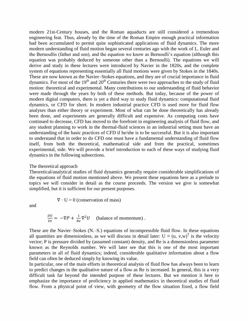
In particular, one of the main efforts in theoretical analysis of fluid flow has always been to learn

to predict changes in the qualitative nature of a flow as Re is increased. In general, this is a very

difficult task far beyond the intended purpose of these lectures. But we mention it here to

emphasize the importance of proficiency in applied mathematics in theoretical studies of fluid

flow. From a physical point of view, with geometry of the flow situation fixed, a flow field

generally becomes ―more complicated‖ as Re increases. This is indicated by the accompanying

time series of a velocity component for three different values of Re. In part (a) of the figure Re is

low, and the flow ultimately becomes time independent. As the Reynolds number is increased to

an intermediate value, the corresponding time series shown in part (b) of the figure is

considerably complicated, but still with evidence of somewhat regular behavior. Finally, in part

(c) is displayed the high-Re case in which the behavior appears to be random. We comment in

passing that it is now known that this behavior is not random, but more appropriately termed

chaotic.

We also point out that the N.–S. equations are widely studied by mathematicians, and they are

said to have been one of two main progenitors of 20th-Century mathematical analysis. (The other

was the Schr¨odinger equation of quantum mechanics.) In the current era it is hoped that such

mathematical analyses will shed some light on the problem of turbulent fluid flow, often termed

―the last unsolved problem of classical mathematical physics.‖ We will from time to time discuss

turbulence in these lectures because most fluid flows are turbulent, and some understanding of it

is essential for engineering analyses. But we will not attempt a rigorous treatment of this topic.

Furthermore, it would not be be possible to employ the level of mathematics used by research

mathematicians in their studies of the N.–S. equations. This is generally too difficult, even for

graduate students.

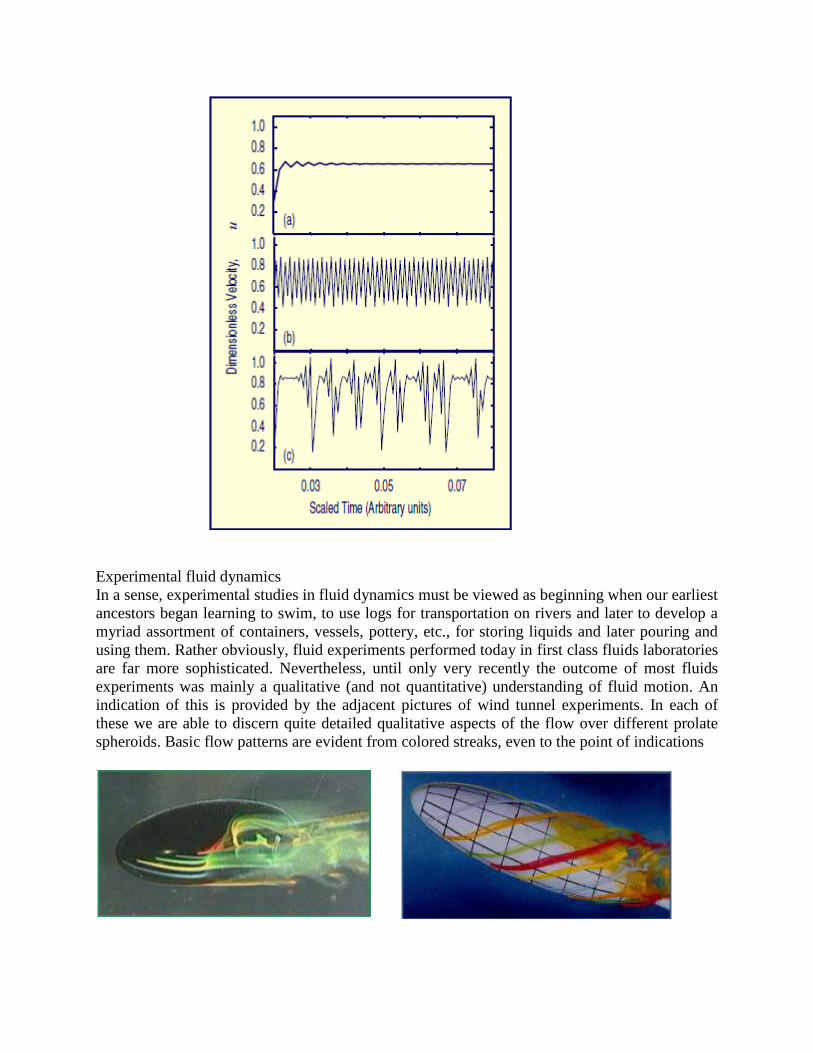
Experimental fluid dynamics

In a sense, experimental studies in fluid dynamics must be viewed as beginning when our earliest

ancestors began learning to swim, to use logs for transportation on rivers and later to develop a

myriad assortment of containers, vessels, pottery, etc., for storing liquids and later pouring and

using them. Rather obviously, fluid experiments performed today in first class fluids laboratories

are far more sophisticated. Nevertheless, until only very recently the outcome of most fluids

experiments was mainly a qualitative (and not quantitative) understanding of fluid motion. An

indication of this is provided by the adjacent pictures of wind tunnel experiments. In each of

these we are able to discern quite detailed qualitative aspects of the flow over different prolate

spheroids. Basic flow patterns are evident from colored streaks, even to the point of indications

of flow ―separation‖ and transition to turbulence. However, such diagnostics provide no

information on actual flow velocity or pressure—the main quantities appearing in the theoretical

equations, and needed for engineering analyses. There have long been methods for measuring

pressure in a flow field, and these could be used simultaneously with the flow visualization of

the above figures to gain some quantitative data. On the other hand, it has been possible to

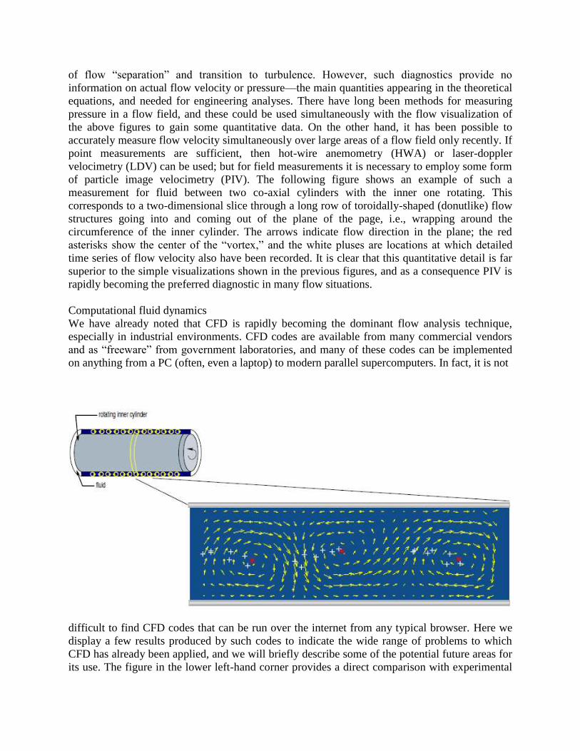
accurately measure flow velocity simultaneously over large areas of a flow field only recently. If

point measurements are sufficient, then hot-wire anemometry (HWA) or laser-doppler

velocimetry (LDV) can be used; but for field measurements it is necessary to employ some form

of particle image velocimetry (PIV). The following figure shows an example of such a

measurement for fluid between two co-axial cylinders with the inner one rotating. This

corresponds to a two-dimensional slice through a long row of toroidally-shaped (donutlike) flow

structures going into and coming out of the plane of the page, i.e., wrapping around the

circumference of the inner cylinder. The arrows indicate flow direction in the plane; the red

asterisks show the center of the ―vortex,‖ and the white pluses are locations at which detailed

time series of flow velocity also have been recorded. It is clear that this quantitative detail is far

superior to the simple visualizations shown in the previous figures, and as a consequence PIV is

rapidly becoming the preferred diagnostic in many flow situations.

Computational fluid dynamics

We have already noted that CFD is rapidly becoming the dominant flow analysis technique,

especially in industrial environments. CFD codes are available from many commercial vendors

and as ―freeware‖ from government laboratories, and many of these codes can be implemented

on anything from a PC (often, even a laptop) to modern parallel supercomputers. In fact, it is not

difficult to find CFD codes that can be run over the internet from any typical browser. Here we

display a few results produced by such codes to indicate the wide range of problems to which

CFD has already been applied, and we will briefly describe some of the potential future areas for

its use. The figure in the lower left-hand corner provides a direct comparison with experimental

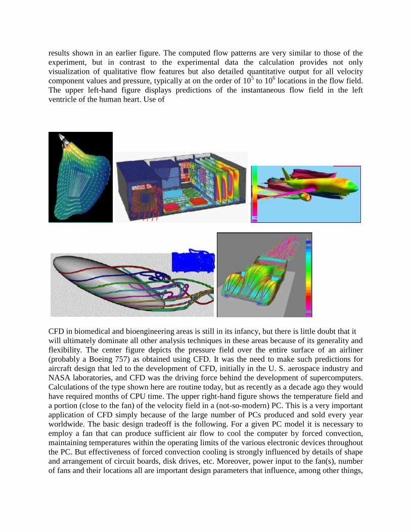
results shown in an earlier figure. The computed flow patterns are very similar to those of the

experiment, but in contrast to the experimental data the calculation provides not only

visualization of qualitative flow features but also detailed quantitative output for all velocity

component values and pressure, typically at on the order of 105 to 10

6 locations in the flow field.

The upper left-hand figure displays predictions of the instantaneous flow field in the left

ventricle of the human heart. Use of

CFD in biomedical and bioengineering areas is still in its infancy, but there is little doubt that it

will ultimately dominate all other analysis techniques in these areas because of its generality and

flexibility. The center figure depicts the pressure field over the entire surface of an airliner

(probably a Boeing 757) as obtained using CFD. It was the need to make such predictions for

aircraft design that led to the development of CFD, initially in the U. S. aerospace industry and

NASA laboratories, and CFD was the driving force behind the development of supercomputers.

Calculations of the type shown here are routine today, but as recently as a decade ago they would

have required months of CPU time. The upper right-hand figure shows the temperature field and

a portion (close to the fan) of the velocity field in a (not-so-modern) PC. This is a very important

application of CFD simply because of the large number of PCs produced and sold every year

worldwide. The basic design tradeoff is the following. For a given PC model it is necessary to

employ a fan that can produce sufficient air flow to cool the computer by forced convection,

maintaining temperatures within the operating limits of the various electronic devices throughout

the PC. But effectiveness of forced convection cooling is strongly influenced by details of shape

and arrangement of circuit boards, disk drives, etc. Moreover, power input to the fan(s), number

of fans and their locations all are important design parameters that influence, among other things,

the unwanted noise produced by the PC. Finally, the lower right-hand figure shows pressure

distribution and qualitative nature of the velocity field for flow over a race car, as computed

using CFD. In recent years CFD has played an ever-increasing role in many areas of sports and

athletics—from study and design of Olympic swimware to the design of a new type of golf ball

providing significantly longer flight times, and thus driving distance (and currently banned by

the PGA). The example of a race car also reflects current heavy use of CFD in numerous areas of

automobile production ranging from the design of modern internal combustion engines

exhibiting improved efficiency and reduced emissions to various aspects of the manufacturing

process, per se, including, for example, spray painting of the completed vehicles. It is essential to

recognize that a CFD computer code solves the Navier–Stokes equations, given earlier, and this

is not a trivial undertaking—often even for seemingly easy physical problems. The user of such

codes must understand the mathematics of these equations sufficiently well to be able to supply

all required auxiliary data for any given problem, and he/she must have sufficient grasp of the

basic physics of fluid flow to be able to assess the outcome of a calculation and determine,

among other things, whether it is ―physically reasonable‖—and if not, decide what to do next.

1.1 What is CFD?

Computational Fluid Dynamics or CFD is the analysis of systems involving fluid flow, heat transfer and associated phenomena such as chemical reactions by means of computer-based simulation. The technique is very powerful and spans a wide range of industrial and non-industrial application areas. Some examples are:

• aerodynamics of aircraft and vehicles: lift and drag • hydrodynamics of ships • power plant: combustion in IC engines and gas turbines • turbomachinery: flows inside rotating passages, diffusers etc. • electrical and electronic engineering: cooling of equipment including microcircuits • chemical process engineering: mixing and separation, polymer moulding • external and internal environment of buildings: wind loading and heating/ ventilation • marine engineering: loads on off-shore structures • environmental engineering: distribution of pollutants and effluents • hydrology and oceanography: flows in rivers, estuaries, oceans • meteorology: weather prediction • biomedical engineering: blood flows through arteries and veins

From the 1960s onwards the aerospace industry has integrated CFD techniques into the design, R&D and manufacture of aircraft and jet engines. More recently the methods have been applied to the design of internal combustion engines, combustion chambers of gas turbines and furnaces. Furthermore, motor vehicle manufacturers now routinely predict drag forces, under-bonnet air flows and the in- car environment with CFD. Increasingly CFD is becoming a vital component in the design of industrial products and processes. The ultimate aim of developments in the CFD field is to provide a capability comparable to other CAE (Computer-Aided Engineering) tools such as stress analysis codes. The main reason why CFD has lagged behind is the tremendous complexity of the underlying behaviour, which precludes a description of fluid flows that is at the same time economical and sufficiently complete. The availability of affordable high performance computing hardware and the introduction of user- friendly interfaces have led to a recent upsurge of

interest and CFD is poised to make an entry into the wider industrial community in the 1990s.

As explained above, flows and related phenomena can be described by partial differential (or

integro-differential) equations, which cannot be solved analytically except in special cases. To

obtain an approximate solution numerically, we have to use a discretization method which

approximates the differential equations by a system of algebraic equations, which can then be

solved on a computer. The approximations are applied to small domains in space and/or time so

the numerical solution provides results at discrete locations in space and time. Much as the

accuracy of experimental data depends on the quality of the tools used, the accuracy of numerical

solutions is dependent on the quality of discretizations used. Contained within the broad field of

computational fluid dynamics are activities that cover the range from the automation of well-

established engineering design methods to the use of detailed solutions of the Navier-Stokes

equations as substitutes for experimental research into the nature of complex flows. CFD is the

numerical solving of partial differential equations on a discretized system that given the

available computer resources best approximates the real geometry and fluid flow phenomena of

interest.

In other words CFD is a tool, similar to experimental tools, used to gain greater physical insight

into problems of interest. Thus, based on

• geometry

• fluid flow physics

• computer

we then select the appropriate:

• governing equations

• numerical method

• grid system

and then examine the results in order to gain physical insight and understanding.

At one end, one can purchase design packages for pipe systems that solve problems in a few

seconds or minutes on personal computers or workstations. On the other, there are codes that

may require hundreds of hours on the largest super-computers. The range is as large as the field

of fluid mechanics itself, making it impossible to cover all of CFD in a single work. Also, the

field is evolving so rapidly that we run the risk of becoming out of date in a short time. CFD is

finding its way into process, chemical, civil, and environmental engineering. Optimization in

these areas can produce large savings in equipment and energy costs and in reduction of

environmental pollution. Clearly the investment costs of a CFD capability are not small, but the total expense is not normally as great as that of a high quality experimental facility. Moreover, there are several unique advantages of CFD over experiment-based approaches to fluid systems design:

• substantial reduction of lead times and costs of new designs • ability to study systems where controlled experiments are difficult or impossible to

perform (e.g. very large systems) • ability to study systems under hazardous conditions at and beyond their normal

performance limits (e.g. safety studies and accident scenarios) • practically unlimited level of detail of results

The variable cost of an experiment, in terms of facility hire and/or man-hour costs, is proportional to the number of data points and the number of configurations tested. In contrast CFD codes can produce extremely large volumes of results at virtually no added expense and it is very cheap to perform parametric studies, for instance to optimise equipment performance.

We also note that, in addition to a substantial investment outlay, an organisation needs qualified

people to run the codes and communicate their results and briefly consider the modelling skills

required by CFD users.

How does a CFD code work?

CFD codes are structured around the numerical algorithms that can tackle fluid flow problems.

In order to provide easy access to their solving power all commercial CFD packages include

sophisticated user interfaces to input problem parameters and to examine the results. Hence all

codes contain three main elements: (i) a pre-processor, (ii) a solver and (iii) a post-processor. We

briefly examine the function of each of these elements within the context of a CFD code.

Pre-processor

Pre-processing consists of the input of a flow problem to a CFD program by means of an

operator-friendly interface and the subsequent transformation of this input into a form suitable

for use by the solver. The user activities at the pre-processing stage involve:

• Definition of the geometry of the region of interest: the computational domain.

• Grid generation-the sub-division of the domain into a number of smaller,

non¬overlapping sub-domains: a grid (or mesh) of cells (or control volumes or elements).

• Selection of the physical and chemical phenomena that need to be modelled.

• Definition of fluid properties.

• Specification of appropriate boundary conditions at cells which coincide with or touch

the domain boundary.

The solution to a flow problem (velocity, pressure, temperature etc.) is defined at nodes inside

each cell. The accuracy of a CFD solution is governed by the number of cells in the grid. In

general, the larger the number of cells the better the solution accuracy. Both the accuracy of a

solution and its cost in terms of necessary computer hardware and calculation time are dependent

on the fineness of the grid. Over 50% of the time spent in industry on a CFD project is devoted

to the definition of the domain geometry and grid generation. In order to maximise productivity

of CFD personnel all the major codes now include their own CAD-style interface and/or

facilities to import data from proprietary surface modellers and mesh generators such as

PATRAN and I-DEAS. Up-to-date pre-processors also give the user access to libraries of

material properties for common fluids and a facility to invoke special physical and chemical

process models (e.g. turbulence models, radiative heat transfer, combustion models) alongside

the main fluid flow equations.

Solver

There are three distinct streams of numerical solution techniques: finite difference, finite element

and spectral methods. In outline the numerical methods that form the basis of the solver perform

the following steps:

• Approximation of the unknown flow variables by means of simple functions.

• Discretisation by substitution of the approximations into the governing flow equations

and subsequent mathematical manipulations.

• Solution of the algebraic equations.

The main differences between the three separate streams are associated with the way in which

the flow variables are approximated and with the discretisation processes. Finite difference

methods. Finite difference methods describe the unknowns <fi of the flow problem by means of

point samples at the node points of a grid of co-ordinate lines. Truncated Taylor series

expansions are often used to generate finite difference approximations of derivatives of (j> in

terms of point samples of cj) at each grid point and its immediate neighbours. Those derivatives

appearing in the governing equations are replaced by finite differences yielding an algebraic

equation for the values of (j> at each grid point. Smith (1985) gives a comprehensive account of

all aspects of the finite difference method.

Finite Element Method. Finite element methods use simple piecewise functions (e.g. linear or

quadratic) valid on elements to describe the local variations of unknown flow variables (j>. The

governing equation is precisely satisfied by the exact solution (p. If the piecewise approximating

functions for (j> are substituted into the equation it will not hold exactly and a residual is defined

to measure the errors. Next the residuals (and hence the errors) are minimised in some sense by

multiplying them by a set of weighting functions and integrating. As a result we obtain a set of

algebraic equations for the unknown coefficients of the approximating functions. The theory of

finite elements has been developed initially for structural stress analysis.

Spectral Methods.

Spectral methods approximate the unknowns by means of truncated Fourier series or series of

Chebyshev polynomials. Unlike the finite difference or finite element approach the

approximations are not local but valid throughout the entire computational domain. Again we

replace the unknowns in the governing equation by the truncated series. The constraint that leads

to the algebraic equations for the coefficients of the Fourier or Chebyshev series is provided by a

weighted residuals concept similar to the finite element method or by making the approximate

function coincide with the exact solution at a number of grid points.

The finite volume method.

The finite volume method was originally developed as a special finite difference formulation.

It is central to four of the five main commercially available CFD codes: PHOENICS, FLUENT,

FLOW3D and STAR-CD. The numerical algorithm consists of the following steps:

• Formal integration of the governing equations of fluid flow over all the (finite) control

volumes of the solution domain.

• Discretisation involves the substitution of a variety of finite-difference-type

approximations for the terms in the integrated equation representing flow processes such as

convection, diffusion and sources. This converts the integral equations into a system of algebraic

equations.

• Solution of the algebraic equations by an iterative method.

The first step, the control volume integration, distinguishes the finite volume method from all

other CFD techniques. The resulting statements express the (exact) conservation of relevant

properties for each finite size cell. This clear relationship between the numerical algorithm and

the underlying physical conservation principle forms one of the main attractions of the finite

volume method and makes its concepts much more simple to understand by engineers than finite

element and spectral methods. The conservation of a general flow variable (j>, for example a

velocity component or enthalpy, within a finite control volume can be expressed as a balance

Basics of Computational Fluid Dynamics

Concept of Computational Fluid Dynamics

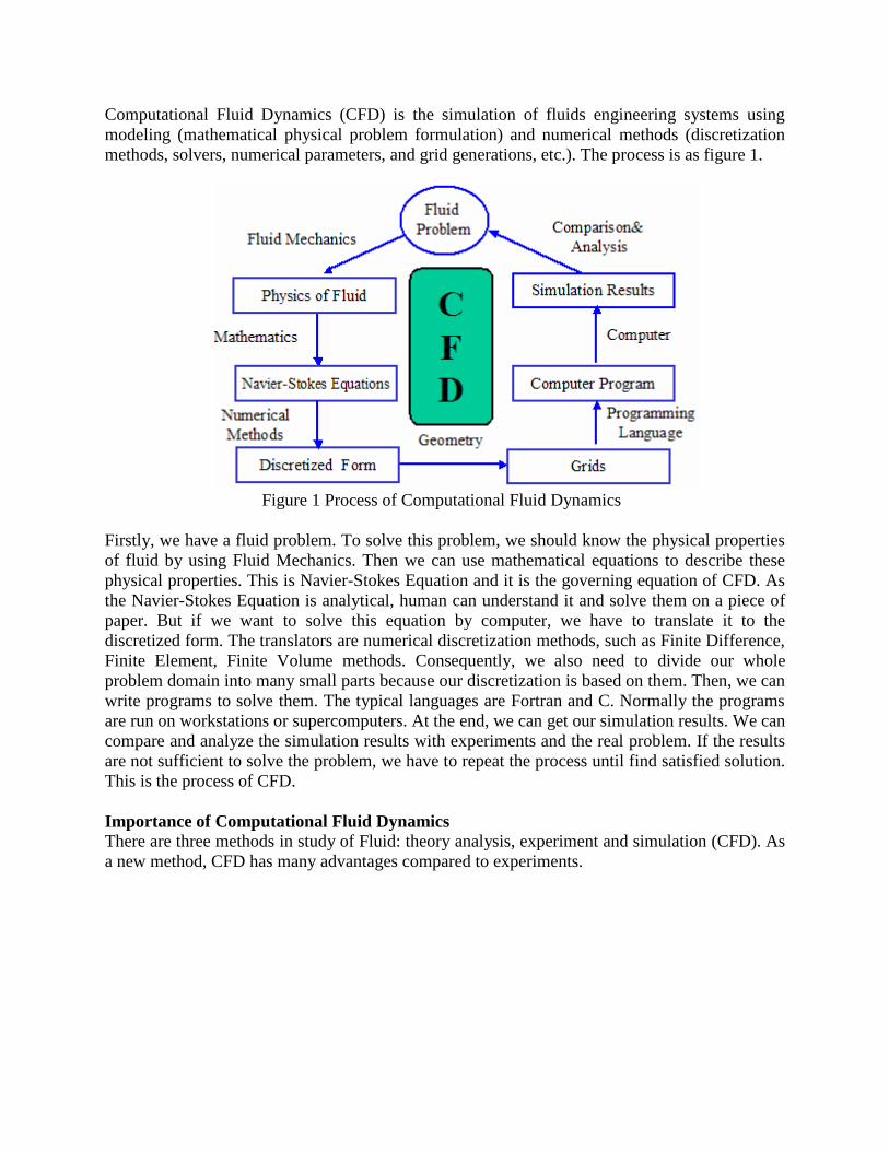
Computational Fluid Dynamics (CFD) is the simulation of fluids engineering systems using

modeling (mathematical physical problem formulation) and numerical methods (discretization

methods, solvers, numerical parameters, and grid generations, etc.). The process is as figure 1.

Figure 1 Process of Computational Fluid Dynamics

Firstly, we have a fluid problem. To solve this problem, we should know the physical properties

of fluid by using Fluid Mechanics. Then we can use mathematical equations to describe these

physical properties. This is Navier-Stokes Equation and it is the governing equation of CFD. As

the Navier-Stokes Equation is analytical, human can understand it and solve them on a piece of

paper. But if we want to solve this equation by computer, we have to translate it to the

discretized form. The translators are numerical discretization methods, such as Finite Difference,

Finite Element, Finite Volume methods. Consequently, we also need to divide our whole

problem domain into many small parts because our discretization is based on them. Then, we can

write programs to solve them. The typical languages are Fortran and C. Normally the programs

are run on workstations or supercomputers. At the end, we can get our simulation results. We can

compare and analyze the simulation results with experiments and the real problem. If the results

are not sufficient to solve the problem, we have to repeat the process until find satisfied solution.

This is the process of CFD.

Importance of Computational Fluid Dynamics

There are three methods in study of Fluid: theory analysis, experiment and simulation (CFD). As

a new method, CFD has many advantages compared to experiments.

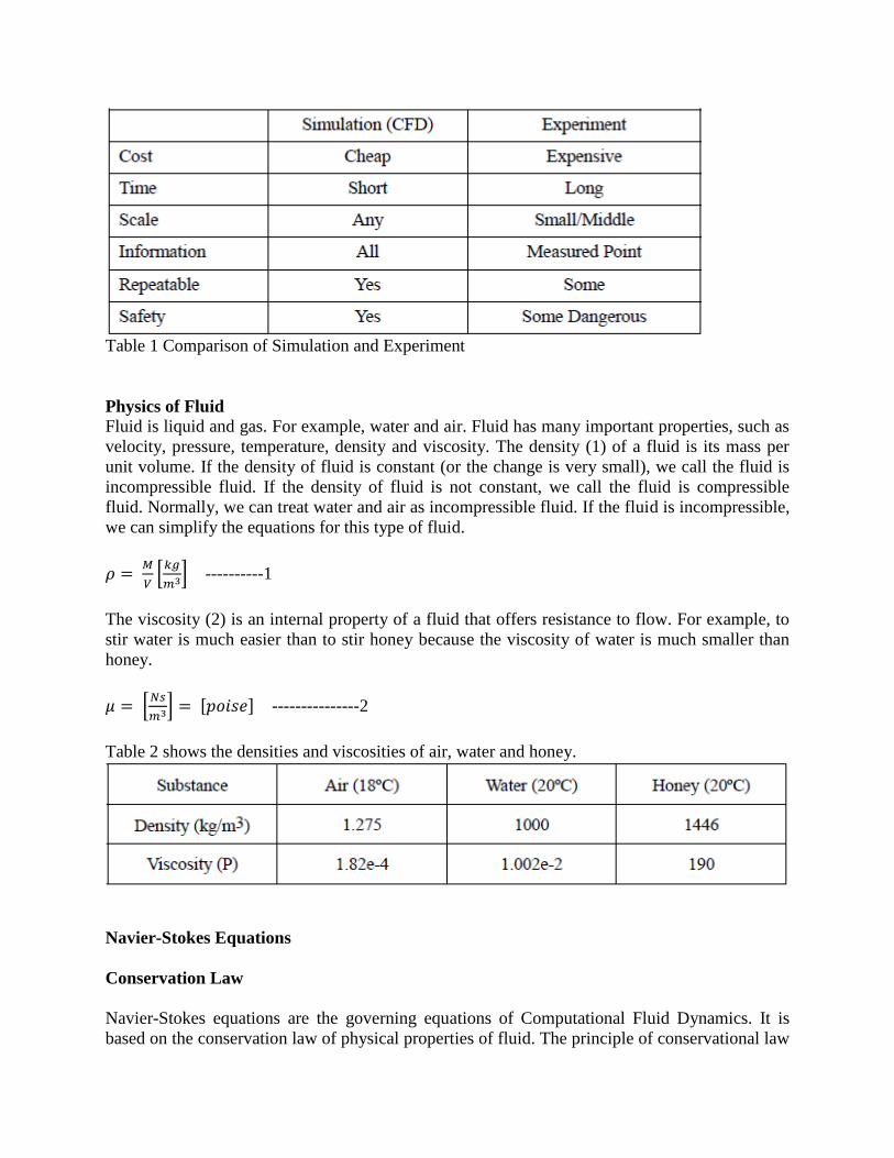
Table 1 Comparison of Simulation and Experiment

Physics of Fluid

Fluid is liquid and gas. For example, water and air. Fluid has many important properties, such as

velocity, pressure, temperature, density and viscosity. The density (1) of a fluid is its mass per

unit volume. If the density of fluid is constant (or the change is very small), we call the fluid is

incompressible fluid. If the density of fluid is not constant, we call the fluid is compressible

fluid. Normally, we can treat water and air as incompressible fluid. If the fluid is incompressible,

we can simplify the equations for this type of fluid.

[

] ----------1

The viscosity (2) is an internal property of a fluid that offers resistance to flow. For example, to

stir water is much easier than to stir honey because the viscosity of water is much smaller than

honey.

[

] [ ] ---------------2

Table 2 shows the densities and viscosities of air, water and honey.

Navier-Stokes Equations

Conservation Law

Navier-Stokes equations are the governing equations of Computational Fluid Dynamics. It is

based on the conservation law of physical properties of fluid. The principle of conservational law

is the change of properties, for example mass, energy, and momentum, in an object is decided by

the input and output.

For example, the change of mass in the object is as follows

--------------3

If = 0, we have

---------------------------4

Which means

M = const ,,,,,,,,,,,,,,,,,,,,,,,,,,,5

Navier-Stokes Equation

Applying the mass, momentum and energy conservation, we can derive the continuity equation,

momentum equation and energy equation as follows.

Continuity Equation

------ 6

Momentum Equation

----------7

Where

(

)

------------- 8

I: Local change with time

II: Momentum convection

III: Surface force

IV: Molecular-dependent momentum exchange (diffusion)

V: Mass force

Energy Equation

------ 9

I : Local energy change with time

II: Convective term

III: Pressure work

IV: Heat flux (diffusion)

V: Irreversible transfer of mechanical energy into heat

If the fluid is compressible, we can simplify the continuity equation and momentum equation as

follows.

Continuity Equation

---------- 10

Momentum Equation

------------ 11

Introduction

Fluid dynamics is a classic discipline. The physical principles governing the flow of simple

fluids and gases, such as water and air, have been understood since the times of Newton. Since

about 1950 classic fluid dynamics finds itself in the company of computational fluid dynamics.

This newer discipline still lacks the elegance and unification of its classic counterpart, and is in a

state of rapid development. The purpose of this lecture note is:

To introduce some notation that will be useful later;

To recall some basic facts of vector analysis;

To introduce the governing equations of laminar incompressible fluid dynamics;

To explain that the Reynolds number is usually very large. In later notes this will be seen

to have a large impact on numerical methods.

What is Computational Fluid Dynamics?

What is CFD? Computational Fluid Dynamics can be defined as the field that uses computer resources to

simulate flow related problems. To simulate a flow problem you have to use mathematical

physical and programming tools to solve the problem then data is generated and analysed. This

field has been developing for the past 30 years. During the last 10 years this field has just made a

big jump especially due to the introduction of new computer hardware and software. University

academics write their own mini sized codes to solve the problems they are usually assigned.

These codes are usually not that user friendly and not very well documented. Before

computational fluid dynamics was used on a wide scale. Engineers had to make small scale

models to validate how slender is their design. A design that is not aerodynamically efficient will

have a negative impact on where the design will be used. So a bad car design will result in more

fuel consumption. While a bad design for a plane might cause it to crash.

Figure 2 : A researcher puts a lorry model inside a wind tunnel for tests. These experiments where done by immersing the model in a transparent fluid/gas and then

applying flow conditions similar to the conditions the model would encounter. Next came was

applying a colour dye to the flow which resulted in showing the flow pattern resulting from the

flow. The set back of using such methods is that after you have got your blue print drawings

from the design team you have to model your design in a work shop. Once the model has been

made you will need to have the experimental set up apparatus in an allocated space in the

engineering lab. Just to note that Wind tunnels are huge in size some of them can contain real

scale model as illustrated in figure 2 below. While now you just need the flow modelling

software, a good research team and lots of computer resources.

Figure 2: A panoramic view of the wind tunnel in the workshops, just to illustrate its

tremendous size in comparison with a desktop computer. The researcher can be seen on the

bottom right hand side of the picture.

The researchers advantage of CFD is that you can have a wind tunnel on your desktop without

having to worry about choosing big fans or that your model will fit into the wind tunnel or not

Figure 3 shows the size extent of a wind tunnel blowing fan. These problems can be solved in the

software by changing the scaling of the studied model or by modifying the value of the inflow

velocity into the studied domain mesh.

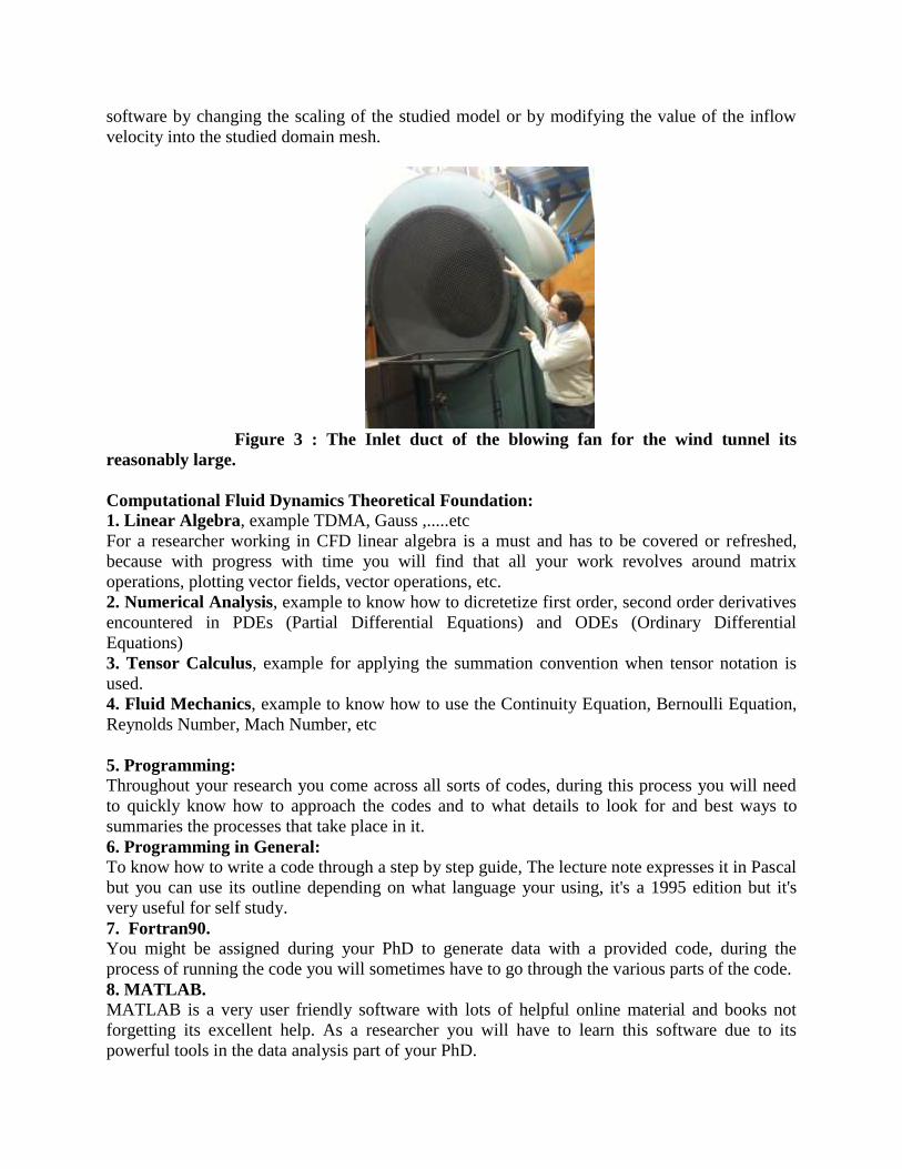
Figure 3 : The Inlet duct of the blowing fan for the wind tunnel its

reasonably large.

Computational Fluid Dynamics Theoretical Foundation: 1. Linear Algebra, example TDMA, Gauss ,.....etc

For a researcher working in CFD linear algebra is a must and has to be covered or refreshed,

because with progress with time you will find that all your work revolves around matrix

operations, plotting vector fields, vector operations, etc.

2. Numerical Analysis, example to know how to dicretetize first order, second order derivatives

encountered in PDEs (Partial Differential Equations) and ODEs (Ordinary Differential

Equations)

3. Tensor Calculus, example for applying the summation convention when tensor notation is

used.

4. Fluid Mechanics, example to know how to use the Continuity Equation, Bernoulli Equation,

Reynolds Number, Mach Number, etc

5. Programming: Throughout your research you come across all sorts of codes, during this process you will need

to quickly know how to approach the codes and to what details to look for and best ways to

summaries the processes that take place in it.

6. Programming in General: To know how to write a code through a step by step guide, The lecture note expresses it in Pascal

but you can use its outline depending on what language your using, it's a 1995 edition but it's

very useful for self study.

7. Fortran90. You might be assigned during your PhD to generate data with a provided code, during the

process of running the code you will sometimes have to go through the various parts of the code.

8. MATLAB. MATLAB is a very user friendly software with lots of helpful online material and books not

forgetting its excellent help. As a researcher you will have to learn this software due to its

powerful tools in the data analysis part of your PhD.

9. Statistics and Probability. If you're going to be working in the field of turbulence you will need statistical tools, while if

you're going to work on reactive flows you will need initially statistical tools and later

probability functions for later stages of your project once you get to the detailed side of

chemistry.

10. Differential Equations and Computational PDEs.

11. Algorithm Theory.

12. Data Structures.

During the research process dealing with all sorts of matrices of different types is an issue that

has to be accepted, depending on the studied problem.

13. Discrete Mathematics.

Steps to Set Up a Simulation During the description of the following, the points might overlap every now and then. Planning

for a simulation is advantageous, it helps you to focus for longer hours, keeps you focused on

your target and confident that you will get to finish on target.

1. Choosing the problem like as case study or in most cases you are assigned a problem which

might represent a air flow in a lecture room or air flow around a car, air flow around a building

...etc.

2. What parameters are of interest. That's if some hints had already been provided by the

manufacturer or by the customer. If the researcher has been assigned the problem and has to start

from scratch this leads him to run simulations for very simple cases , then to verify that the

results if they are correct by comparing the data with experimental or available literature data.

Once this objective is achieved the researcher would select the required parameters for study,

makes a list of them and then starts running more detailed simulations. What is meant if we are

interested in combustion case turbulence intensity is an attractive parameter to study which

means it can illustrate the magnitude of mixing strength in the process. Another parameter to

study and can give a good indication of the rate of mixing is through plotting the eddy viscosity

frequency. Shear strain rate can give a good indication on flow break up leading to dissipation

such an example is a jet blowing into a stagnant air in a room.

3. The user has to specify if it’s an Internal flow case (looking at figure 4 which represents a

throttle valve) or an external flow case (looking at figure 5 which refers to a wind turbine).

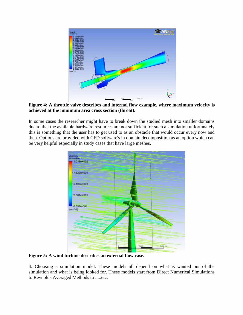
Figure 4: A throttle valve describes and internal flow example, where maximum velocity is

achieved at the minimum area cross section (throat).

In some cases the researcher might have to break down the studied mesh into smaller domains

due to that the available hardware resources are not sufficient for such a simulation unfortunately

this is something that the user has to get used to as an obstacle that would occur every now and

then. Options are provided with CFD software's in domain decomposition as an option which can

be very helpful especially in study cases that have large meshes.

Figure 5: A wind turbine describes an external flow case.

4. Choosing a simulation model. These models all depend on what is wanted out of the

simulation and what is being looked for. These models start from Direct Numerical Simulations

to Reynolds Averaged Methods to .....etc.

5. Assessing the required hardware and software resources and what is available. Due to these

challenges the user has to take into account these issues as an example simulation run time,

calculation time on the desktop, data storage and simulation grid resolution, how many cores are

required ....etc.

6. Specifing the boundary conditions in the simulation. These can refer to solid walls or inflow

and outflow boundaries. At some cases moving boundaries are taken into account as cases in

simulating flows in pumps, compressors, wind turbines ....etc. At certain cases the smoothness of

the boundaries have to be specified as smooth or rough boundaries.

7. Selecting the physical continuum which might be Air, Argon, Nitrogen, .......etc.

8. Selecting a Mesh type for the simulation. Will it be hexahedral or tri-diagonal ...etc. Usually

CFD software has several meshing options to choose from.

Mathematical Flow Modelling On the assumption that the problem is a flow problem:

1. Choosing the coordinates system, which specifies what space the student, will work on.

Metric, Soblove or Hillbert space..etc. At later stages this will lead the researcher to adopt

specified mathematical methods that can only be used in these spaces.

2. Choosing the reference coordinate system, this is automatically taken at point (0,0,0) . The

equations that you are going to solved are related to the coordinate system for the space relation.

Once motion is going to be studied that means we will have a generated mesh velocity and

acceleration to be taken in account. The use of velocity acceleration leads to the conclusion that

derivatives are going to be used. Once derivatives come into account that means at later stages

we will need to use some kind of discretization method.

3. The studied domain geometry and dimensions. Is it a box, rectangular, sphere or cylinder or a

complex domain?. This relates to the required scales to be captured by the simulation. Another

factor is the studied object. As an example the Navier-Stokes equations are applicable at certain

length ranges at small scales Lattice-Boltzman might be better at a smaller scale schrodinger

equation that all depends on using the Knudsen number to verify the scale of the studied case.

4. Then comes how many species will there be? in most case air is taken as the studied fluid.

That will ease the studied case. While if several species are taken into account will complicate

the study more. Several species will lead us to two cases either a reactive or a non-reactive case.

5. Compressible or non compressible fluid case. Each case has a different approach to solve the

major difference is in how to solve the pressure problem. In compressible flows you just use the

ideal gas equation while in incompressible flows you will need to use a more complex approach

for it.

6. Choosing the physical governing laws of importance. Will it be a Conservation of momentum

or Conservation of mass or Conservation of energy or all at the same time?

7. Choosing thermodynamic reference parameters temperature, viscosity, pressure, this is

essential, because at certain occasions due to that some parameters change in relation to other

parameters , as an example viscosity is related to temperature using the Sutherland formula.

8. Now we are ready to Choose a Numerical Model. A quick survey on the available models

their pros and cons. Usually you can find a researcher who had already done this in a recently

published paper if your studied case is not that recent then look for a book that has summarised

the models. At really advanced stages you might have to make your own model which is very

hard not forgetting it’s not easy to convince people to use your model except if it's something

really outstanding.

9. None dimensionlizing process of the used equations where required, this always gives the

written code a more dynamic characteristic to use the code on a wider spectrum of problems.

Equations Used (Numerical Method) All the equations used in the study of flows are derived from Reynolds Transport Theory, it is

recommended to memories this equation and from it derive all the forms you want to study.

From it you can derive the continuity equation, the momentum equations, the species equation

and finally the energy equation (in the case of working with compressible gases new quantities

will be added to the study such as the adiabatic equation). You can add as many quantities to

your studied case by using the Reynolds Transport Theory keeping in mind the computer

resource that are available for the researcher.

The Navier-Stokes Equations are used, that’s in general term, in detail the researcher can think of

these equations as representing the motion of a particle in space. Using CFD the splitting of a

predefined space into small cells and using the Navier-Stokes Equations for each studied cell.

People usual feel scared from the term equations and once derivatives and lots of them are used

that quickly lead to a quick decision i can’t understand it i won’t read it. Actually these set of

equations represent the change of a vector quantity in 3D space, the vector quantity in the Stokes

equation is the velocity vector. The Stokes equations represent the transfer of momentum in a

studied flow.

∫

∫ ( ) ∫ ( ) ∫

simplifying the equation to a form that is related to a regular uniform mesh gives

( ) ( )

applying would lead to the continuity equation

( )

Once you write down the set of equations you will be using for your study, the next step is to see

what forces are wanted to be taken into account and what factors will be neglected in the study.

This will lead the researcher to the available models for his study which starts with DNS (Direct

Numerical Analysis and finishes with simple models) the selection of the model depends on the

studied case from one perspective and available recourses from another perspective.

so for a case of studying the transport of the scalar quantity of velocity in the y axis direction we

would assign the value which results in the following formula:

( ) ( )

while for a case of studying the transport of the scalar quantity of temperature in the studied

domain we would assign the value which results in the following formula:

( ) ( )

so for a case of studying the transport of the scalar quantity of species in the studied domain we

would assign the value which is called a volume fraction which results in the

following formula.

( ) ( )

A CFD code consist of the following parts: Just as a way to make things clear for the reader you can think of a CFD parts as a Human body

where input parameters are food to be eaten, the time discretization section is the humans head,

the space discretization section is the human body. While the computer compiler represents the

heart.

1. Input Parameters:

This section holds the number of grid points in the domain, domain dimensions, initialization

profile selection, and simulation time length. As a researcher you would be working most of the

time on the input file changing different variables and then running a simulation. At more

advanced stages of PhD you would have to write your own subroutines and add them to the code.

2. Time Discretization Section:

The two mostly liked methods that are used in CFD, are the Runge-Kutta and Crank Nicholson

Method. If the code uses the Runge-Kutta method the time stepping section forms a mostly

independent section of the code while using the crank Nicholson Method you will find there is a

more strong coupling between the time and space discretization parts of the code. Codes usually

have a criteria to run a simulation where after each calculated time step the code checks that the

simulation stays stable. In such cases there are some formulas that are used to satisfy the

condition in having the best discrete time to achieve a stable simulation.

3. Space Discretization Section:

Space discretization consist of the next four parts, these four parts are essential and cannot be

neglect, because each one is related to the other and has a direct impact to the other.

a. Grid Generation.

A grid has to be generated and depending to the type of fluid it will be chosen. as an example the

use of staggered grid in incompressible gases. Some people would say why is the grid so

important. Once you start the analysis process you will need to see the values of the studied

scalar at the generated points. This is done through plotting the vector fields or plotting contour

plot ....etc. Some time you will need to see the value of velocity at a certain part of the domain.

In such a case you will just give the coordinates of the point to extract its value

b. Initialization Profiles.

You can run a simulation without having an initialization profile but its side effects that you will

need several thousand time steps till the flow develops into its predicted form depending on the

simulation stop criteria. Explicit or implicit methods are also related to initialization for space

discretization and time.

c. Boundary Conditions.

During a fluid flow simulation you always need to assign a certain surface some inflow

parameters and another one at least to be outflow surface. You can specify that be assigning a

source term a value of flow velocity .The choice of periodic condition or none periodic depends

on your requirements. Periodic satisfies a condition where at each time step of the simulation the

amount of flow into the domain is the same as the amount of going out of the domain. Choosing

surface roughness is also a requirement.

d. Discretization Methods.

There are various discretization schemes they start with very simple once such as central

differencing scheme which requires two points and can end with schemes that use more than 15

grid points.

4. Output Section:

This is the section usually the researcher is assigned to. The researcher has to read the output

data into a visualization software such as Tecplot, MATLAB, Excel....etc. Usually the code

generates a set of output files these files have the calculated sets of data like the grid reference

number its coordinates the value of the velocity at the point its temperature its pressure ...etc.

Skills for Building a Code: 1. To build a working numerical model that gives you data output which is not necessary correct

is done using random number generators. This can also be accomplished using straight forward

numbers such as 1.

2. Checking the physical units of the formula that they are homogenous.

3. Once you get the code working without bugs, next comes validation of data output. This is

done by seeing experimental plots our published tables of the studied quantity.

What's an Equation? An equation is a mathematical expression that represents a region of points in a certain space.

The researcher has to choose the range of study to specify his data matrix dimensions. Once the

known's are specified for the studied case then comes writing the mathematical formula into a

way the programming language interprets it to the computer. This is done by taking the formula

apart depending on the number of variables and assigning them suitable names.Then comes

specifying the number of points required. This is mostly done based on computer resources and

how much is the required accuracy.