Computational Biomechanics 2016

Lecture I:

Introduction,

Basic Mechanics 1

Ulli Simon, Frank Niemeyer, Martin Pietsch

Scientific Computing Centre Ulm, UZWR Ulm University

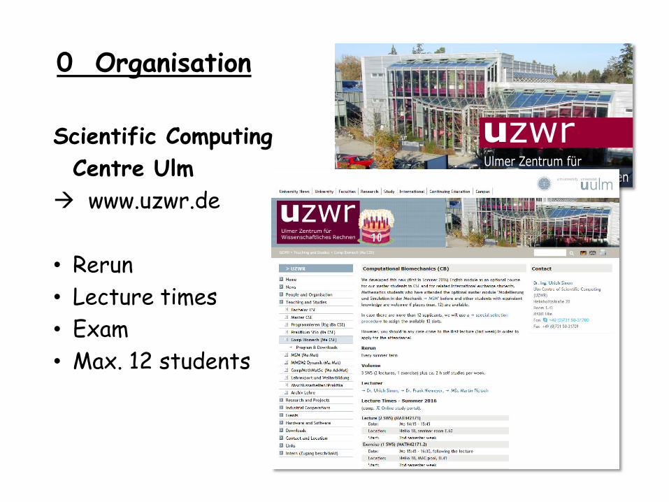
Scientific Computing

Centre Ulm

www.uzwr.de

• Rerun

• Lecture times

• Exam

• Max. 12 students

0 Organisation

Computational

Biomechanics

Biology

Mechanics

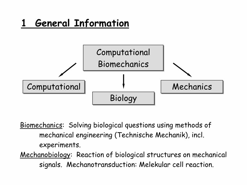
1 General Information

Computational

Biomechanics: Solving biological questions using methods of

mechanical engineering (Technische Mechanik), incl.

experiments.

Mechanobiology: Reaction of biological structures on mechanical

signals. Mechanotransduction: Melekular cell reaction.

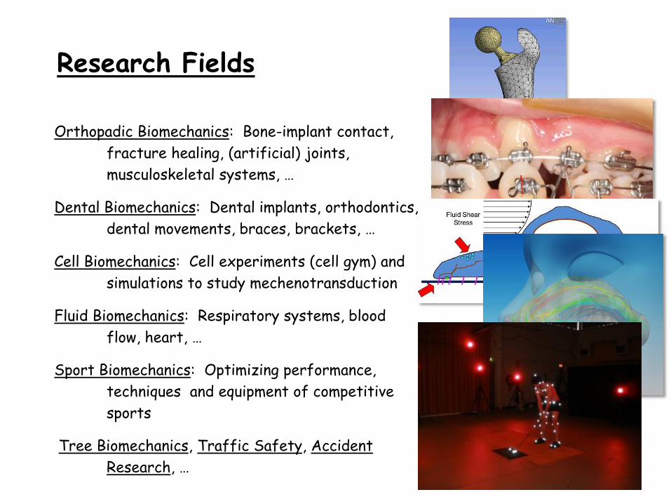
Research Fields

Orthopadic Biomechanics: Bone-implant contact,

fracture healing, (artificial) joints,

musculoskeletal systems, …

Dental Biomechanics: Dental implants, orthodontics,

dental movements, braces, brackets, …

Cell Biomechanics: Cell experiments (cell gym) and

simulations to study mechenotransduction

Fluid Biomechanics: Respiratory systems, blood

flow, heart, …

Sport Biomechanics: Optimizing performance,

techniques and equipment of competitive

sports

Tree Biomechanics, Traffic Safety, Accident

Research, …

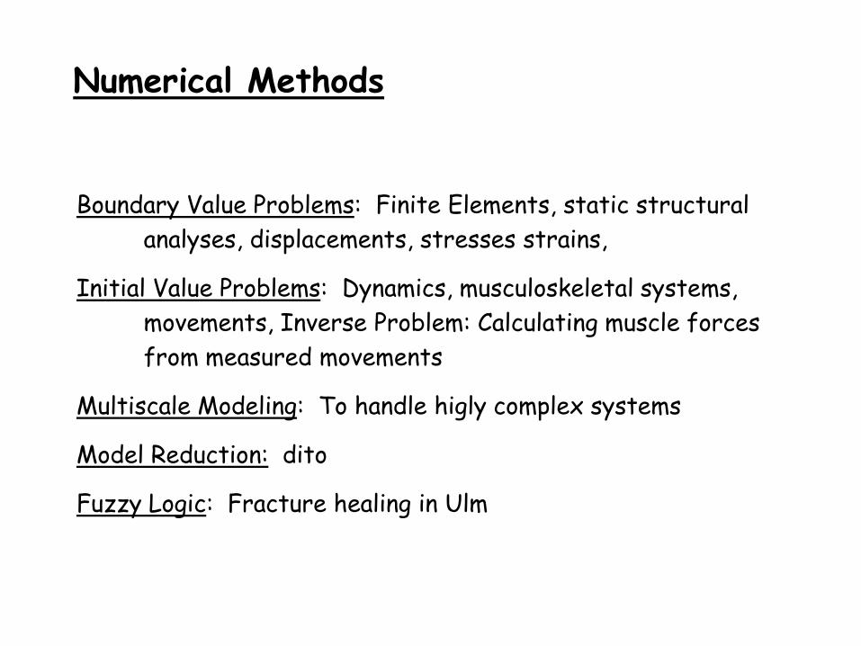
Numerical Methods

Boundary Value Problems: Finite Elements, static structural

analyses, displacements, stresses strains,

Initial Value Problems: Dynamics, musculoskeletal systems,

movements, Inverse Problem: Calculating muscle forces

from measured movements

Multiscale Modeling: To handle higly complex systems

Model Reduction: dito

Fuzzy Logic: Fracture healing in Ulm

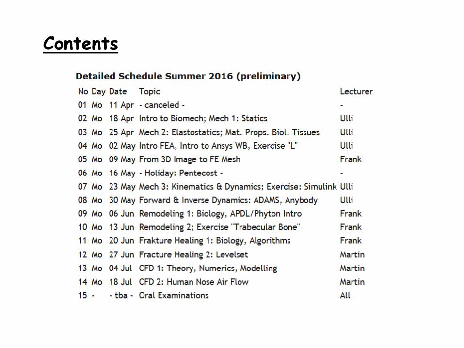
Contents

Appetizer:

Simulation of Bone Healing

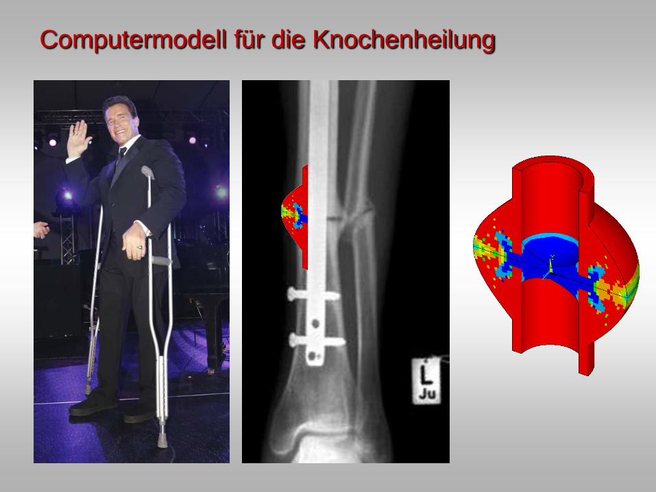
Computermodell für die Knochenheilung

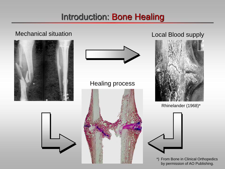
Introduction: Bone Healing

Healing process

Mechanical situation Local Blood supply

Rhinelander (1968)*

*) From Bone in Clinical Orthopedics

by permission of AO Publishing.

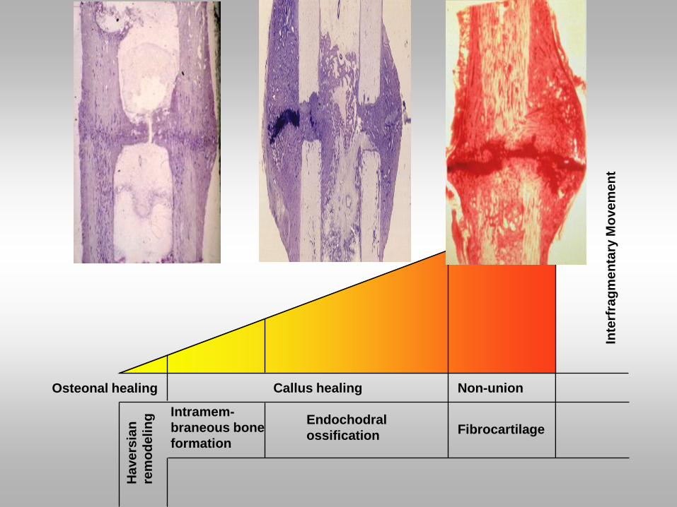
Osteonal healing Callus healing Non-union

Intramem-

braneous bone

formation

Havers

ian

rem

od

eli

ng

Endochodral

ossification Fibrocartilage

Inte

rfra

gm

en

tary

Mo

ve

me

nt

QuickTime™ und der

Foto-CD-Dekompressor

werden benötigt, um dieses Bild zu sehen.

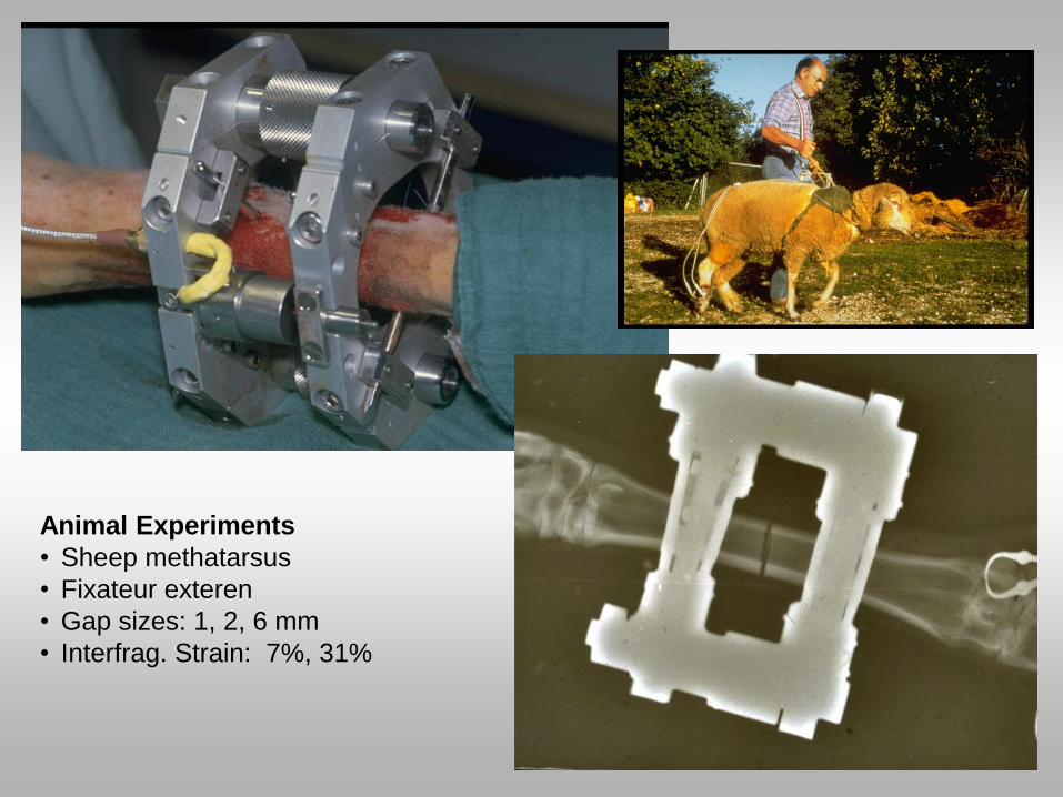
Animal Experiments

• Sheep methatarsus

• Fixateur exteren

• Gap sizes: 1, 2, 6 mm

• Interfrag. Strain: 7%, 31%

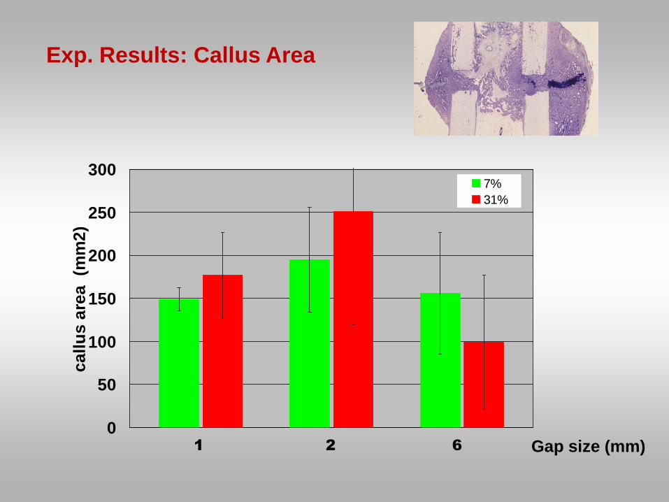
Exp. Results: Callus Area

0

50

100

150

200

250

300

ca

llu

s a

rea

(m

m2

)

7%

31%

1 Gap size (mm) 1 2 6

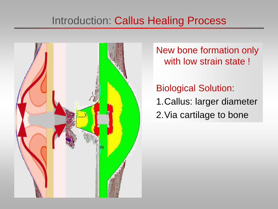
Introduction: Callus Healing Process

New bone formation only

with low strain state !

Biological Solution:

1.Callus: larger diameter

2.Via cartilage to bone

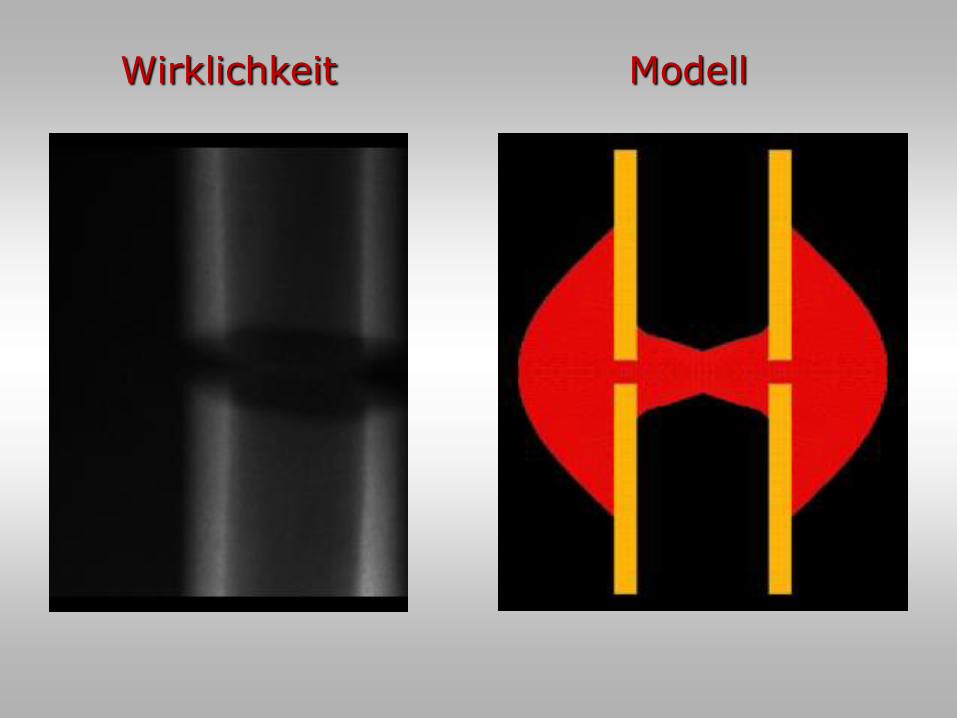
Wirklichkeit Modell

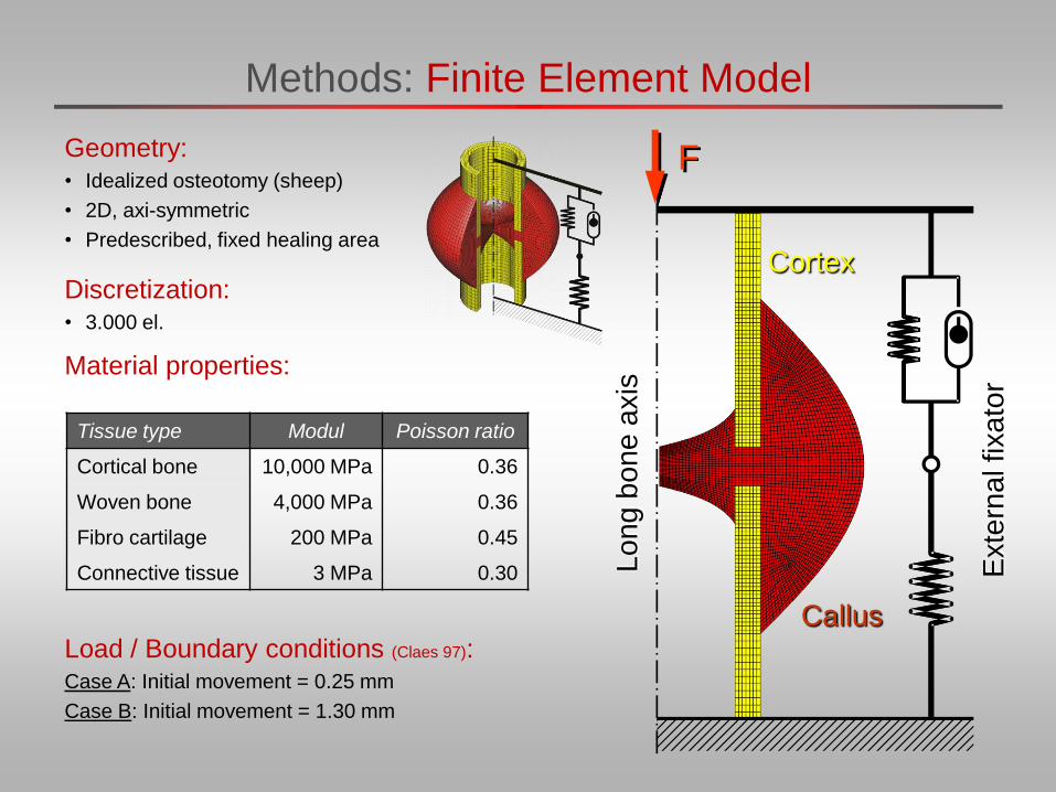
Geometry: • Idealized osteotomy (sheep)

• 2D, axi-symmetric

• Predescribed, fixed healing area

Discretization: • 3.000 el.

Material properties:

Load / Boundary conditions (Claes 97): Case A: Initial movement = 0.25 mm

Case B: Initial movement = 1.30 mm

Tissue type Modul Poisson ratio

Cortical bone 10,000 MPa 0.36

Woven bone 4,000 MPa 0.36

Fibro cartilage 200 MPa 0.45

Connective tissue 3 MPa 0.30

Methods: Finite Element Model

F

Exte

rna

l fixa

tor

Callus

Cortex

Lo

ng

bo

ne

axis

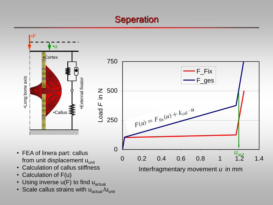
Seperation

0

250

500

750

0 0.2 0.4 0.6 0.8 1 1.2 1.4

Interfragmentary movement u in mm

Lo

ad

F in N

F_Fix

F_ges

•F

•Exte

rna

l fixa

tor

•Callus

•Cortex

•Lo

ng b

on

e a

xis

• •u

• FEA of linera part: callus

from unit displacement uunit

• Calculation of callus stiffness

• Calculation of F(u)

• Using inverse u(F) to find uactual

• Scale callus strains with uactual /uunit

uact

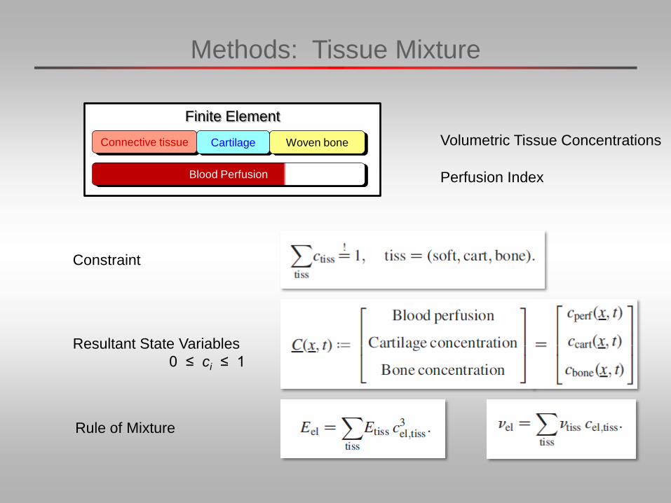
Finite Element

Connective tissue Cartilage Woven bone

Blood Perfusion

Methods: Tissue Mixture

Rule of Mixture

Constraint

Resultant State Variables

0 ≤ ci ≤ 1

Volumetric Tissue Concentrations

Perfusion Index

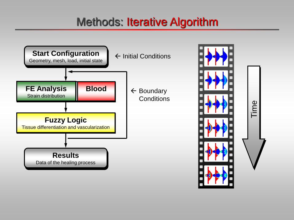
Tim

e

Results Data of the healing process

FE Analysis Strain distribution

Fuzzy Logic Tissue differentiation and vascularization

Start Configuration Geometry, mesh, load, initial state

Blood

Methods: Iterative Algorithm

Initial Conditions

Boundary

Conditions

Methods: Tissue Healing with Fuzzy Logic

Fuzzy Controler with linguistic rules

Vasc. adjacent

Bone concentration

Change of

Vascularity

Input variables Output variables

dilatational strain

distortional strain

Vascularity

Bone conc. adjacent

Change of

cartilage concentr.

Cartilage concentr.

Change of

bone concentration

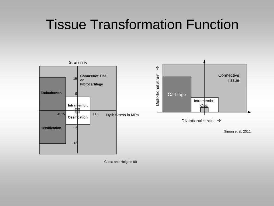
Tissue Transformation Function

Strain in %

Hydr.Stress in MPa

Connective Tiss.

or

Fibrocartilage

Endochondr.

Ossification

-0.15 0.15

15

5

-5

-15

Intramembr..

Ossification

Claes and Heigele 99

Cartilage

Dis

tort

iona

l str

ain

Connective

Tissue

Intramembr.

Oss.

Dilatational strain

Simon et al. 2011

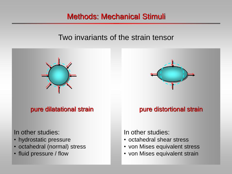
pure distortional strain

In other studies: • octahedral shear stress

• von Mises equivalent stress

• von Mises equivalent strain

pure dilatational strain

In other studies: • hydrostatic pressure

• octahedral (normal) stress

• fluid pressure / flow

Methods: Mechanical Stimuli

Two invariants of the strain tensor

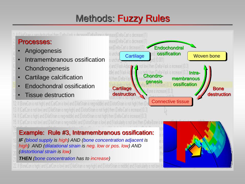
Processes:

• Angiogenesis

• Intramembranous ossification

• Chondrogenesis

• Cartilage calcification

• Endochondral ossification

• Tissue destruction

Chondro-

genesis

Connective tissue

Cartilage

Bone

destruction

Cartilage

destruction

Intra-

membranous

ossification

Woven bone

Endochondral

ossification

Example: Rule #3, Intramembranous ossification: IF (blood supply is high) AND (bone concentration adjacent is

high) AND (dilatational strain is neg. low or pos. low) AND

(distortional strain is low)

THEN (bone concentration has to increase)

Methods: Fuzzy Rules

0

0,5

1

0,0001 0,001 0,01 0,1 1

distortional strain

pro

ba

bilit

y

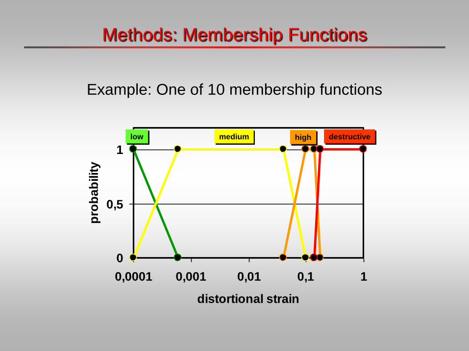
Methods: Membership Functions

low medium high

Example: One of 10 membership functions

destructive

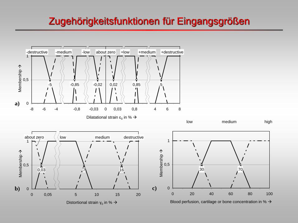
Zugehörigkeitsfunktionen für Eingangsgrößen

30 70

0

0,5

1

0 20 40 60 80 100

Blood perfusion, cartilage or bone concentration in %

Me

mb

ers

hip

Mem

bers

hip

Blood perfusion, cartilage or bone concentration in %

medium high low

-0,02 0,02

0

0,5

1

-0,12 -0,09 -0,06 -0,03 0 0,03 0,06 0,09 0,12

dilatational strain

me

mb

ers

hip

-0,85 -0,020,02 0,85

0

0,5

1

-1,2 -0,8 -0,4 0 0,4 0,8 1,2

dilatational strain

me

mb

ers

hip

-0,85 -0,020,02 0,85

0

0,5

1

-1,2 -0,8 -0,4 0 0,4 0,8 1,2

dilatational strain

me

mb

ers

hip

-0,85-0,020,020,85 5-5

0

0,5

1

-8 -6 -4 -2 0 2 4 6 8

dilatational strain

me

mb

ers

hip

-0,85-0,020,020,85 5-5

0

0,5

1

-8 -6 -4 -2 0 2 4 6 8

dilatational strain

me

mb

ers

hip

Mem

bers

hip

Dilatational strain ε0 in %

+medium +destructive about zero +low -destructive -medium -low

a)

0,03

0

0,5

1

0 0,05 0,1 0,15 0,2 0,25 0,3

distortional strain in %

pro

ba

bili

ty

0,03 7 16

0

0,5

1

-5 0 5 10 15 20

distortional strain in %

pro

ba

bili

ty

medium destructive about zero low

Distortional strain γ0 in %

Mem

bers

hip

b) c)

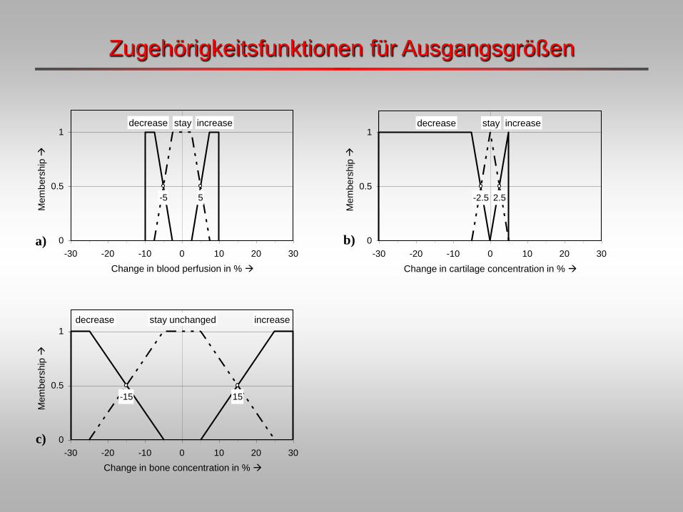
Zugehörigkeitsfunktionen für Ausgangsgrößen

-5 5

0

0.5

1

-30 -20 -10 0 10 20 30

Change in blood perfusion in %

Me

mb

ers

hip

stay increase decrease

a)

Mem

bers

hip

Change in blood perfusion in %

-2.5 2.5

0

0.5

1

-30 -20 -10 0 10 20 30

Change in cartilage concentration in %

Me

mb

ers

hip

stay increase decrease

b)

Mem

bers

hip

Change in cartilage concentration in %

-15 15

0

0.5

1

-30 -20 -10 0 10 20 30

Change in bone concentration in %

Me

mb

ers

hip

stay unchanged increase decrease

c)

Mem

bers

hip

Change in bone concentration in %

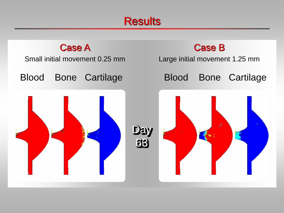
Case B Large initial movement 1.25 mm

Case A Small initial movement 0.25 mm

Results

Blood Bone Cartilage Blood Bone Cartilage

Day

0

Day

7

Day

14

Day

21

Day

28

Day

35

Day

42

Day

49

Day

56

Day

63

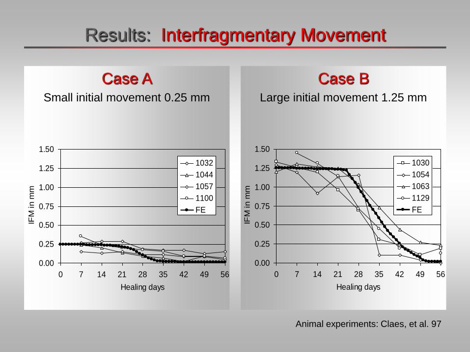
Case B Large initial movement 1.25 mm

Case A Small initial movement 0.25 mm

Results: Interfragmentary Movement

0.00

0.25

0.50

0.75

1.00

1.25

1.50

0 7 14 21 28 35 42 49 56

Healing days

IFM

in

mm

1032

1044

1057

1100

FE

0.00

0.25

0.50

0.75

1.00

1.25

1.50

0 7 14 21 28 35 42 49 56

Healing days

IFM

in

mm

1030

1054

1063

1129

FE

Animal experiments: Claes, et al. 97

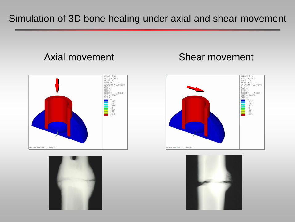
Shear movement Axial movement

Simulation of 3D bone healing under axial and shear movement

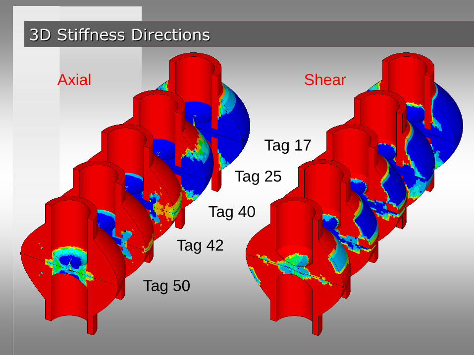
Tag 17

Tag 25

Tag 40

Tag 42

Tag 50

3D Stiffness Directions

Axial Shear

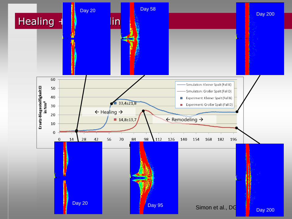
Simon et al., DGfB, Münster 2009

Healing + Remodeling

Day 95

Day 58 Day 20

Day 20

Day 200

Day 200

Remodeling

Healing

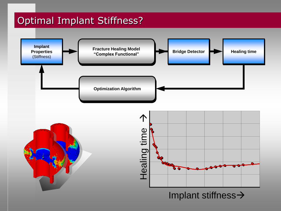
Optimal Implant Stiffness?

Fracture Healing Model

“Complex Functional”

Implant

Properties (Stiffness)

Healing time

Optimization Algorithm

Bridge Detector

Implant stiffness

Hea

ling t

ime

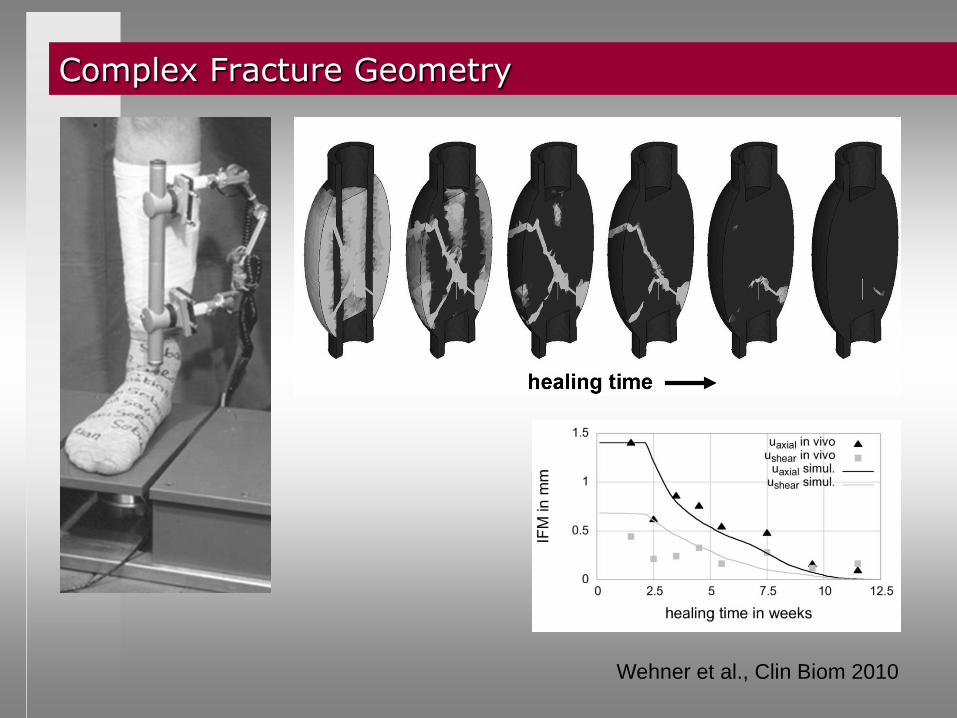
Complex Fracture Geometry

Wehner et al., Clin Biom 2010

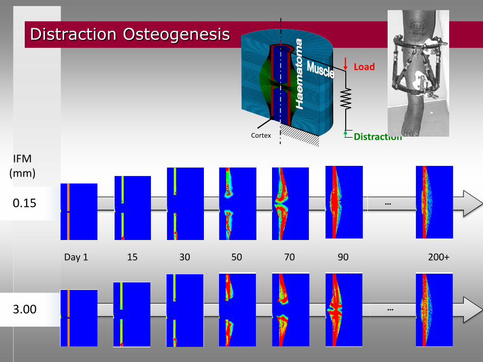
IFM (mm)

0.15

3.00

…

…

Day 1 15 30 50 70 90 200+

Cortex Distraction

Load

Distraction Osteogenesis

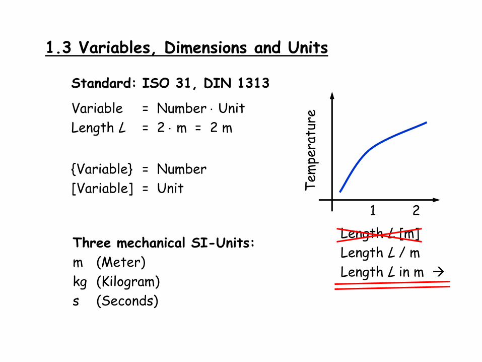
1.3 Variables, Dimensions and Units

Standard: ISO 31, DIN 1313

Variable = Number Unit

Length L = 2 m = 2 m

{Variable} = Number

[Variable] = Unit

Three mechanical SI-Units:

m (Meter)

kg (Kilogram)

s (Seconds)

Length L [m]

Length L / m

Length L in m

2 1

Tem

pera

ture

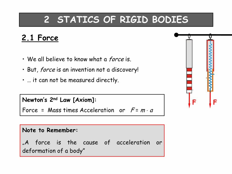
Note to Remember:

„A force is the cause of acceleration or

deformation of a body”

Newton’s 2nd Law [Axiom]:

Force = Mass times Acceleration or F = m a

• We all believe to know what a force is.

• But, force is an invention not a discovery!

• … it can not be measured directly.

2.1 Force

2 STATICS OF RIGID BODIES

F F

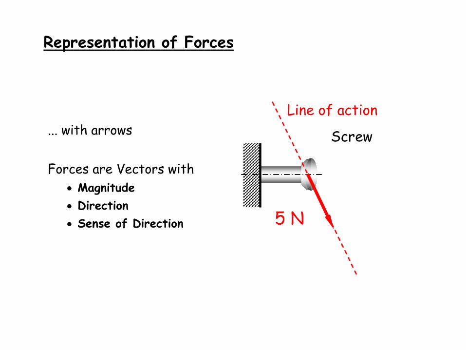
... with arrows

Forces are Vectors with

Magnitude

Direction

Sense of Direction

Representation of Forces

5 N

Line of action

Screw

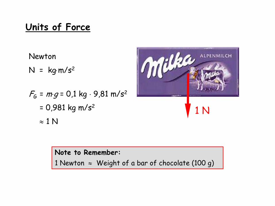
Units of Force

Newton

N = kgm/s2

1 N

Note to Remember:

1 Newton Weight of a bar of chocolate (100 g)

FG = mg = 0,1 kg 9,81 m/s2

= 0,981 kg m/s2

1 N

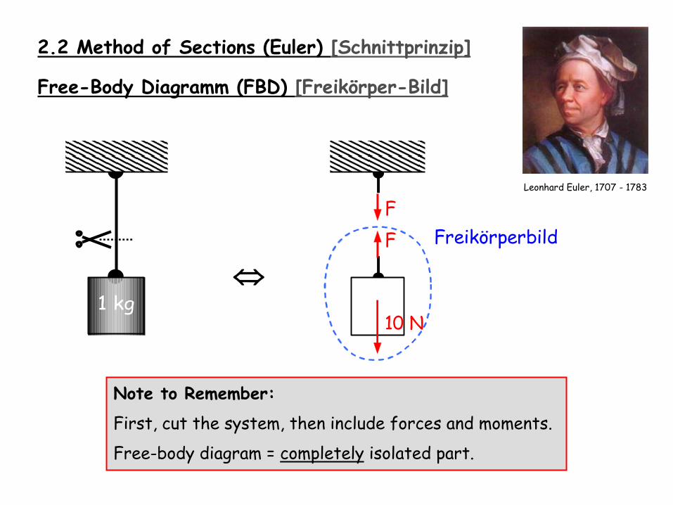
2.2 Method of Sections (Euler) [Schnittprinzip]

Note to Remember:

First, cut the system, then include forces and moments.

Free-body diagram = completely isolated part.

Free-Body Diagramm (FBD) [Freikörper-Bild]

Leonhard Euler, 1707 - 1783

1 kg

F

F

Freikörperbild

10 N

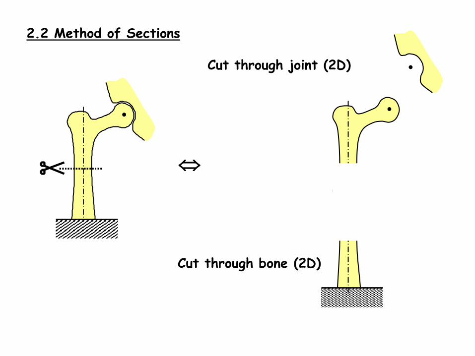
Cut through bone (2D)

Cut through joint (2D)

2.2 Method of Sections

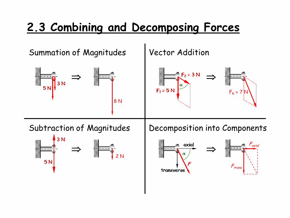
2.3 Combining and Decomposing Forces

Summation of Magnitudes

Subtraction of Magnitudes

Decomposition into Components

Vector Addition

8 N

2 N

FR 7 N

Ftrans

Faxial

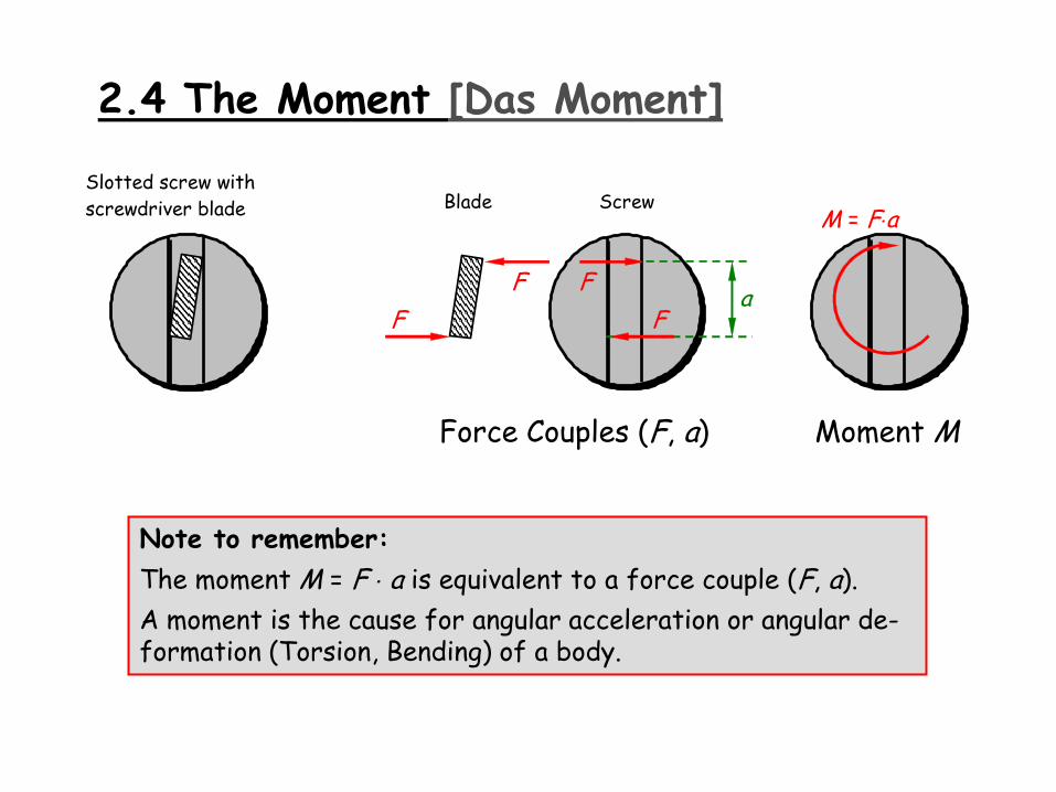
2.4 The Moment [Das Moment]

Note to remember:

The moment M = F a is equivalent to a force couple (F, a).

A moment is the cause for angular acceleration or angular de-formation (Torsion, Bending) of a body.

Screw Blade

Slotted screw with

screwdriver blade M = Fa

Force Couples (F, a) Moment M

F

F a

F

F

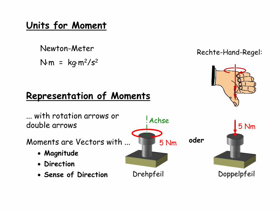
Units for Moment

Newton-Meter

Nm = kgm2/s2

Representation of Moments

... with rotation arrows or double arrows

Moments are Vectors with ...

Magnitude

Direction

Sense of Direction

Rechte-Hand-Regel:

5 Nm

Achse

Drehpfeil

5 Nm

Doppelpfeil

oder

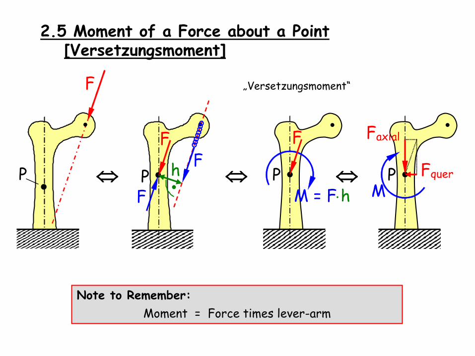
2.5 Moment of a Force about a Point [Versetzungsmoment]

Note to Remember:

Moment = Force times lever-arm

F

P

P M = Fh

F

F

h P

P M

Faxial

Fquer

F

F

„Versetzungsmoment“

2.7 Static Equilibrium

Important:

Free-body diagram (FBD) first, then equilibrium!

For 2D Problems max. 3 equations for each FBD:

(For 3D Problems max. 6 equations for each FBD)

F

F

10 N

Free-body diagram

(FBD)

The sum of all forces in x-direction equals zero:

The sum of all forces in y-direction equals zero:

The sum of Moments with respect to P equals zero:

0...!

,2,1 yy FF

0...!

,2,1 P

z

P

z MM

0...!

,2,1 xx FF

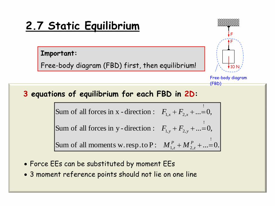
.0...:P toresp. w.moments all of Sum

,0...:direction-yin forces all of Sum

,0...:direction-in x forces all of Sum

!

,2,1

!

,2,1

!

,2,1

P

z

P

z

yy

xx

MM

FF

FF

Force EEs can be substituted by moment EEs

3 moment reference points should not lie on one line

3 equations of equilibrium for each FBD in 2D:

2.7 Static Equilibrium

Important:

Free-body diagram (FBD) first, then equilibrium!

F

F

10 N

Free-body diagram

(FBD)

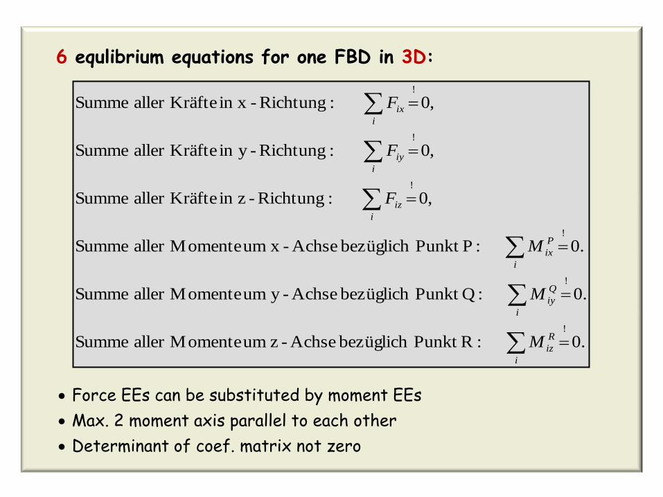
.0 :RPunkt bezüglich Achse-z um Momentealler Summe

.0 :QPunkt bezüglich Achse-y um Momentealler Summe

.0 :PPunkt bezüglich Achse- xum Momentealler Summe

,0 :Richtung-zin Kräftealler Summe

,0 :Richtung-yin Kräftealler Summe

,0 :Richtung-in x Kräftealler Summe

!

!

!

!

!

!

i

R

iz

i

Q

iy

i

P

ix

i

iz

i

iy

i

ix

M

M

M

F

F

F

6 equlibrium equations for one FBD in 3D:

Force EEs can be substituted by moment EEs

Max. 2 moment axis parallel to each other

Determinant of coef. matrix not zero

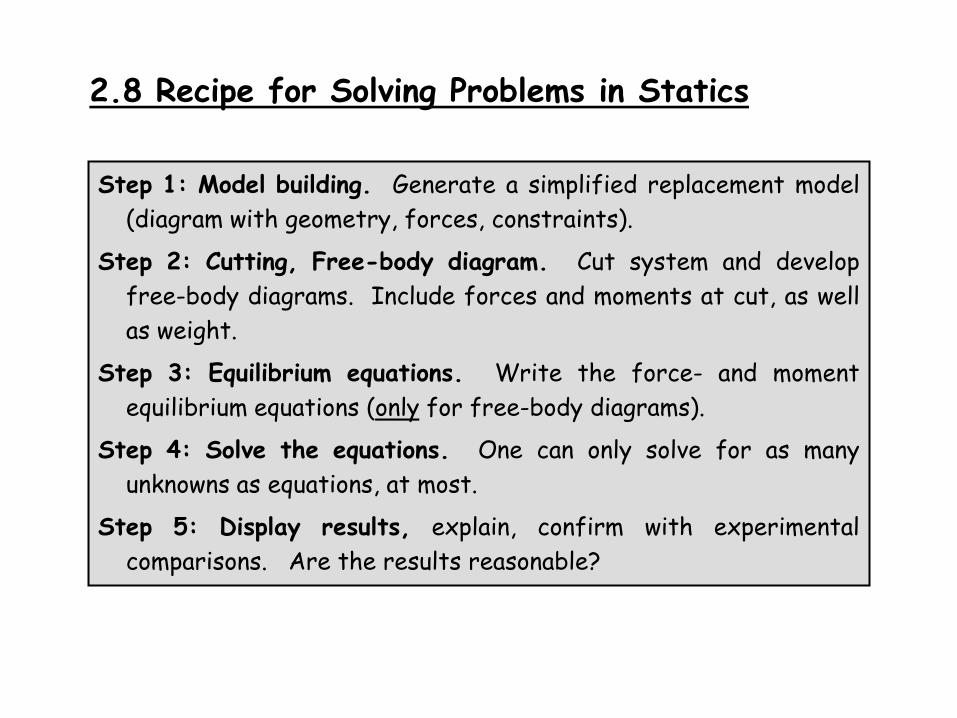
2.8 Recipe for Solving Problems in Statics

Step 1: Model building. Generate a simplified replacement model

(diagram with geometry, forces, constraints).

Step 2: Cutting, Free-body diagram. Cut system and develop

free-body diagrams. Include forces and moments at cut, as well

as weight.

Step 3: Equilibrium equations. Write the force- and moment

equilibrium equations (only for free-body diagrams).

Step 4: Solve the equations. One can only solve for as many

unknowns as equations, at most.

Step 5: Display results, explain, confirm with experimental

comparisons. Are the results reasonable?