Embed Size (px)
Citation preview
Lecture I : An introduction to periodic Chern insulators
Gianluca Panati
Dipartimento di Matematica
Università di Roma La Sapienza
based on joint work withD. Fiorenza (Roma 1) and D. Monaco (SISSA)
The Mathematics of Topological Insulators in Naplesorganized within the Cond-Math project, www.cond-math.it

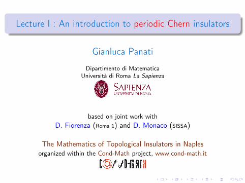
Collaborators
Domenico Fiorenza
(La Sapienza, Roma).
Domenico Monaco
(SISSA, Trieste).
Collaborators
Domenico Fiorenza
(La Sapienza, Roma).Domenico Monaco
(SISSA, Trieste).
Introduction and overview
1869: Mendeleev’s periodic table
Dmitri Ivanovich Mendeleev (1834-1907)
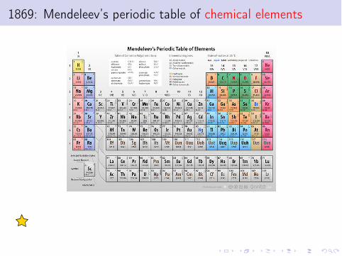
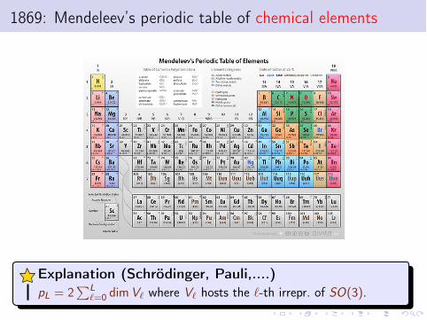
1869: Mendeleev’s periodic table of chemical elements
Classification & quantitative information
The integers pL
2 {2, 8, 18, 32} play a special rôle.
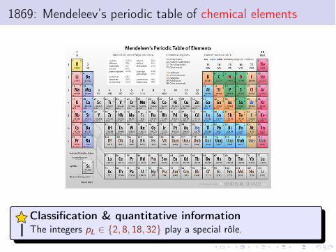
1869: Mendeleev’s periodic table of chemical elements
Classification & quantitative information
The integers pL
2 {2, 8, 18, 32} play a special rôle.
1869: Mendeleev’s periodic table of chemical elements
Explanation (Schrödinger, Pauli,....)
pL
= 2P
L
`=0
dim V` where V` hosts the `-th irrepr. of SO(3).
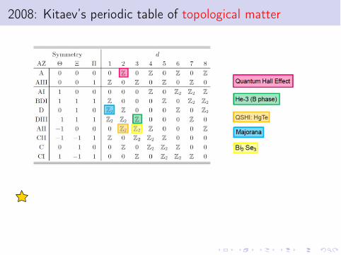
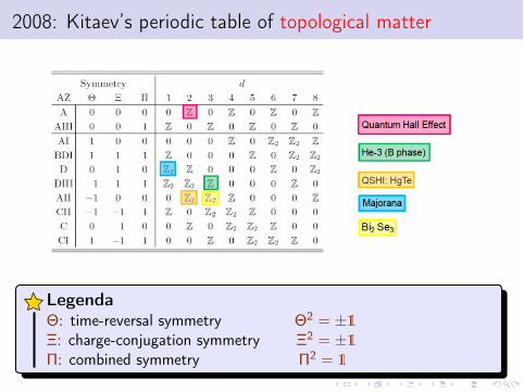
2008: Kitaev’s periodic table of topological matter
Legenda
⇥: time-reversal symmetry ⇥2 = ±1⌅: charge-conjugation symmetry ⌅2 = ±1⇧: combined symmetry ⇧2 = 1
2008: Kitaev’s periodic table of topological matter
Legenda
⇥: time-reversal symmetry ⇥2 = ±1⌅: charge-conjugation symmetry ⌅2 = ±1⇧: combined symmetry ⇧2 = 1
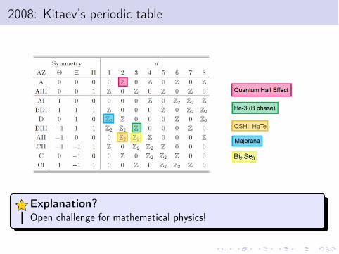
2008: Kitaev’s periodic table
Explanation?
Open challenge for mathematical physics!
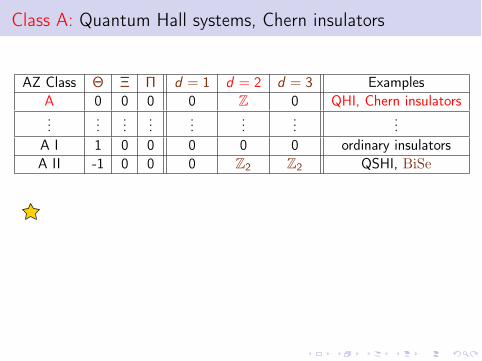
Class A: Quantum Hall systems, Chern insulators
AZ Class ⇥ ⌅ ⇧ d = 1 d = 2 d = 3 ExamplesA 0 0 0 0 Z 0 QHI, Chern insulators...
......
......
......
...A I 1 0 0 0 0 0 ordinary insulatorsA II -1 0 0 0 Z
2
Z2
QSHI, BiSe
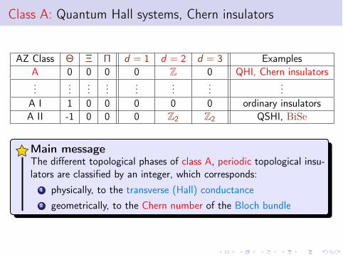
Main message
The different topological phases of class A, periodic topological insu-lators are classified by an integer, which corresponds:
1 physically, to the transverse (Hall) conductance2 geometrically, to the Chern number of the Bloch bundle
Class A: Quantum Hall systems, Chern insulators
AZ Class ⇥ ⌅ ⇧ d = 1 d = 2 d = 3 ExamplesA 0 0 0 0 Z 0 QHI, Chern insulators...
......
......
......
...A I 1 0 0 0 0 0 ordinary insulatorsA II -1 0 0 0 Z
2
Z2
QSHI, BiSe
Main message
The different topological phases of class A, periodic topological insu-lators are classified by an integer, which corresponds:
1 physically, to the transverse (Hall) conductance2 geometrically, to the Chern number of the Bloch bundle
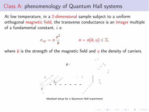
Class A: phenomenology of Quantum Hall systems
At low temperature, in a 2-dimensional sample subject to a uniformorthogonal magnetic field, the transverse conductance is an integer multipleof a fundamental constant, i. e.
�xy
= ne2
hn = n(b, ⌘) 2 Z,
where b is the strength of the magnetic field and ⌘ the density of carriers.
Idealized setup for a Quantum Hall experiment
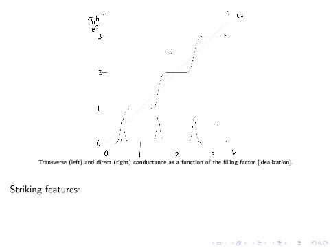
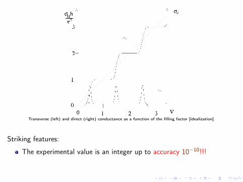
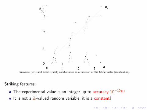
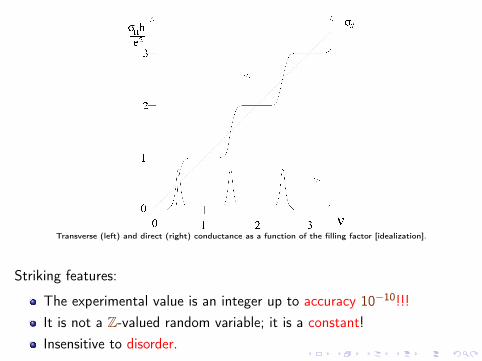
Transverse (left) and direct (right) conductance as a function of the filling factor [idealization].
Striking features:
The experimental value is an integer up to accuracy 10�10!!!It is not a Z-valued random variable; it is a constant!Insensitive to disorder.
Transverse (left) and direct (right) conductance as a function of the filling factor [idealization].
Striking features:
The experimental value is an integer up to accuracy 10�10!!!It is not a Z-valued random variable; it is a constant!Insensitive to disorder.
Transverse (left) and direct (right) conductance as a function of the filling factor [idealization].
Striking features:
The experimental value is an integer up to accuracy 10�10!!!It is not a Z-valued random variable; it is a constant!Insensitive to disorder.
Transverse (left) and direct (right) conductance as a function of the filling factor [idealization].
Striking features:
The experimental value is an integer up to accuracy 10�10!!!It is not a Z-valued random variable; it is a constant!Insensitive to disorder.
Class A: phenomenology of Chern insulators
As conjectured by Haldane [Hal 88], the transverse conductance might benon-zero even without external magnetic fields. The time-reversalsymmetry is broken at the microscopic level.The materials exhibiting this behaviour are called Chern insulators.
Plan of the course: Lecture I
Lecture I - An introduction to periodic Chern insulatorsSymmetry class A: broken TR-symmetry, broken PH-symmetryExamples: Quantum Hall systems, Chern insulators. Crucial: d = 2
1. Periodic Schrödinger operators breaking the TR-symmetry1.1 A continuous model �! diagonalization by Bloch-Floquet transform1.2 Essential structure: a smooth covariant family of projectors
2. The Bloch bundle and its (first) Chern class2.1 Geometric insight: the Bloch bundle2.2 Obstruction to the existence of a continuous Bloch frame [d = 2]:
the Chern number
3. Is the Chern number observable? [! Lectures by G.M. Graf]
Plan of the course: Lecture II
Lecture II - An introduction to periodic TRS topological insulatorsSymmetry class A II: broken PH-symmetryExamples: artificial crystalline solids in dimension d 2 {2, 3}
1. Periodic Schrödinger operators with TR-symmetry1.1 TR-symmetry in classical and quantum mechanics: even & odd case1.2 Covariant families of projectors with TR-symmetry: even & odd case
2. Existence of continuous TR-symmetric Bloch frames?2.1 Key formula 1: Obstruction as a winding number2.3 Comparison with the Fu-Kane-Mele formula2.3 A glimpse to higher-dimensional cases
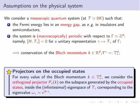
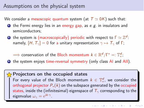
Assumptions on the physical system
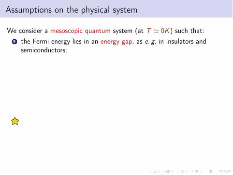
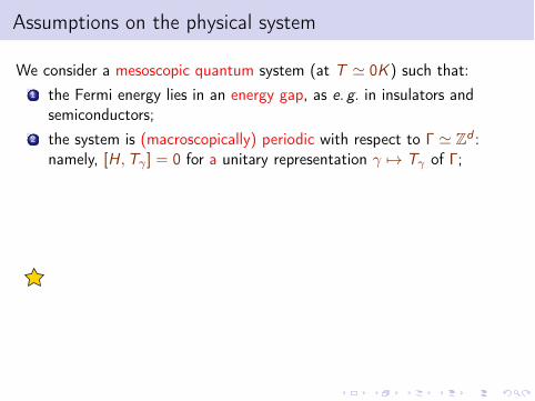
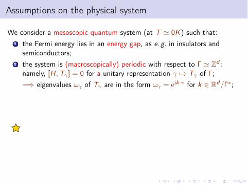
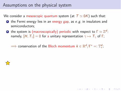
We consider a mesoscopic quantum system (at T ' 0K ) such that:1 the Fermi energy lies in an energy gap, as e. g. in insulators and
semiconductors;2 the system is (macroscopically) periodic with respect to � ' Zd :
namely, [H,T� ] = 0 for a unitary representation � 7! T� of �;=) eigenvalues !� of T� are in the form !� = eik·� for k 2 Rd/�⇤;=) conservation of the Bloch momentum k 2 Rd/�⇤ =: Td⇤ ;
3 the system enjoys time-reversal symmetry (only class AI and AII).
Projectors on the occupied states
For every value of the Bloch momentum k 2 Td⇤ , we consider theorthogonal projector P⇤(k) on the subspace generated by the occupiedstates, inside the (infinitesimal) eigenspace of T� corresponding to theeigenvalue !� = eik·� .
Assumptions on the physical system
We consider a mesoscopic quantum system (at T ' 0K ) such that:1 the Fermi energy lies in an energy gap, as e. g. in insulators and
semiconductors;2 the system is (macroscopically) periodic with respect to � ' Zd :
namely, [H,T� ] = 0 for a unitary representation � 7! T� of �;=) eigenvalues !� of T� are in the form !� = eik·� for k 2 Rd/�⇤;=) conservation of the Bloch momentum k 2 Rd/�⇤ =: Td⇤ ;
3 the system enjoys time-reversal symmetry (only class AI and AII).
Projectors on the occupied states
For every value of the Bloch momentum k 2 Td⇤ , we consider theorthogonal projector P⇤(k) on the subspace generated by the occupiedstates, inside the (infinitesimal) eigenspace of T� corresponding to theeigenvalue !� = eik·� .
Section 1Periodic Schrödinger operators
breaking the TR-symmetry
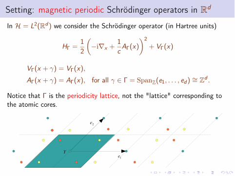
Setting: magnetic periodic Schrödinger operators in Rd
In H = L2(Rd ) we consider the Schrödinger operator (in Hartree units)
H� =12
✓
�irx
+1cA�(x)
◆
2
+ V�(x)
V�(x + �) = V�(x),
A�(x + �) = A�(x), for all � 2 � = SpanZ(e1
, . . . , ed
) ⇠= Zd .
Notice that � is the periodicity lattice, not the "lattice" corresponding tothe atomic cores.
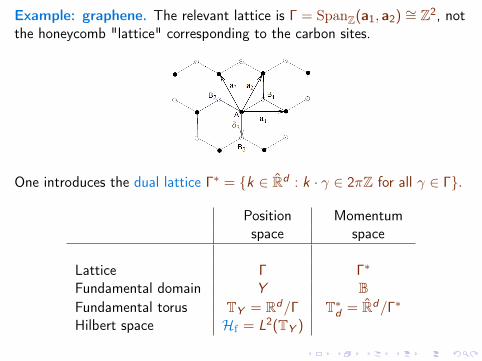
Example: graphene. The relevant lattice is � = SpanZ(a1
, a2
) ⇠= Z2, notthe honeycomb "lattice" corresponding to the carbon sites.
One introduces the dual lattice �⇤ = {k 2 R̂d : k · � 2 2⇡Z for all � 2 �}.
Position Momentumspace space
Lattice � �⇤
Fundamental domain Y BFundamental torus T
Y
= Rd/� T⇤d
= R̂d/�⇤
Hilbert space Hf
= L2(TY
)
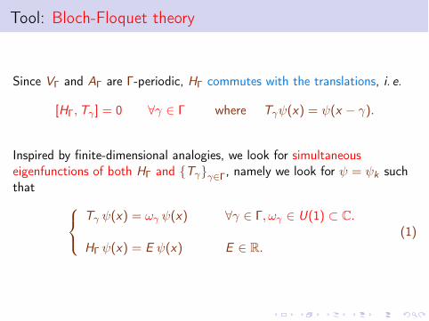
Tool: Bloch-Floquet theory
Since V� and A� are �-periodic, H� commutes with the translations, i. e.
[H�,T� ] = 0 8� 2 � where T� (x) = (x � �).
Inspired by finite-dimensional analogies, we look for simultaneouseigenfunctions of both H� and {T�}�2�, namely we look for =
k
suchthat
8
<
:
T� (x) = !� (x) 8� 2 �,!� 2 U(1) ⇢ C.
H� (x) = E (x) E 2 R.(1)
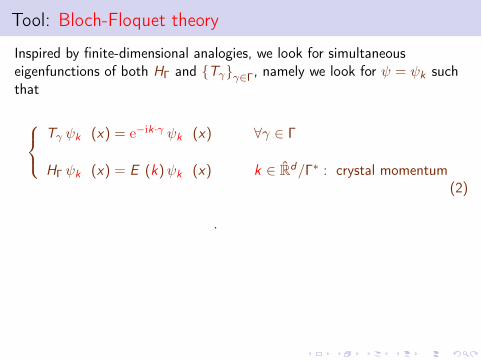
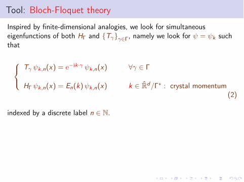
Tool: Bloch-Floquet theory
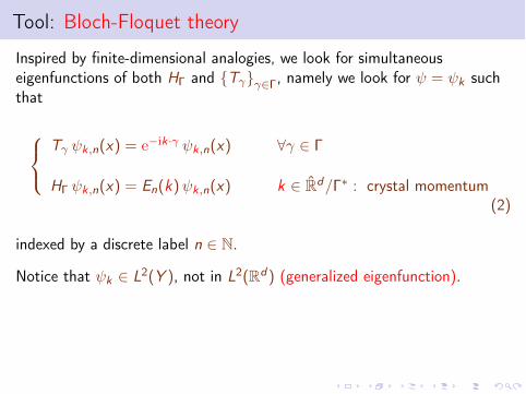
Inspired by finite-dimensional analogies, we look for simultaneouseigenfunctions of both H� and {T�}�2�, namely we look for =
k
suchthat
8
<
:
T� k,n(x) = e�ik·�
k,n(x) 8� 2 �
H� k,n(x) = E
n
(k) k,n(x) k 2 R̂d/�⇤ : crystal momentum
(2)
indexed by a discrete label n 2 N.
Notice that k
2 L2(Y ), not in L2(Rd ) (generalized eigenfunction).
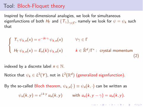
By the so-called Bloch theorem, k,n(·) ⌘
n
(k , ·) can be written as
n
(k , y) = ei k·y un
(k , y) with un
(k , y � �) = un
(k , y).
Tool: Bloch-Floquet theory
Inspired by finite-dimensional analogies, we look for simultaneouseigenfunctions of both H� and {T�}�2�, namely we look for =
k
suchthat
8
<
:
T� k,n(x) = e�ik·�
k,n(x) 8� 2 �
H� k,n(x) = E
n
(k) k,n(x) k 2 R̂d/�⇤ : crystal momentum
(2)
indexed by a discrete label n 2 N.
Notice that k
2 L2(Y ), not in L2(Rd ) (generalized eigenfunction).
By the so-called Bloch theorem, k,n(·) ⌘
n
(k , ·) can be written as
n
(k , y) = ei k·y un
(k , y) with un
(k , y � �) = un
(k , y).
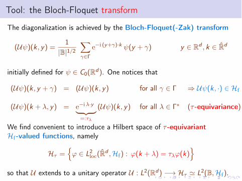
Tool: the Bloch-Floquet transform
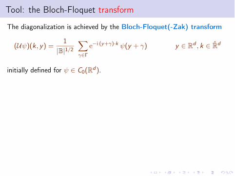
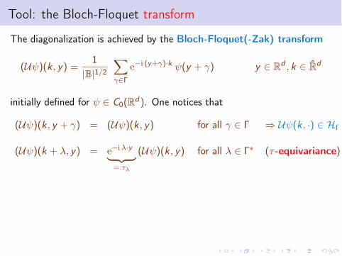
The diagonalization is achieved by the Bloch-Floquet(-Zak) transform
(U )(k , y) = 1|B|1/2
X
�2�e�i (y+�)·k (y + �) y 2 Rd , k 2 R̂d
initially defined for 2 C0
(Rd ). One notices that
(U )(k , y + �) = (U )(k , y) for all � 2 � ) U (k , ·) 2 Hf
(U )(k + �, y) = e�i�·y || {z }
=:⌧�
(U )(k , y) for all � 2 �⇤ (⌧ -equivariance)
We find convenient to introduce a Hilbert space of ⌧ -equivariant
Hf
-valued functions, namely
H⌧ =n
' 2 L2
loc
(R̂d ,Hf
) : '(k + �) = ⌧�'(k)o
so that U extends to a unitary operator U : L2(Rd ) �! H⌧ ' L2(B,Hf
).
Tool: the Bloch-Floquet transform
The diagonalization is achieved by the Bloch-Floquet(-Zak) transform
(U )(k , y) = 1|B|1/2
X
�2�e�i (y+�)·k (y + �) y 2 Rd , k 2 R̂d
initially defined for 2 C0
(Rd ). One notices that
(U )(k , y + �) = (U )(k , y) for all � 2 � ) U (k , ·) 2 Hf
(U )(k + �, y) = e�i�·y || {z }
=:⌧�
(U )(k , y) for all � 2 �⇤ (⌧ -equivariance)
We find convenient to introduce a Hilbert space of ⌧ -equivariant
Hf
-valued functions, namely
H⌧ =n
' 2 L2
loc
(R̂d ,Hf
) : '(k + �) = ⌧�'(k)o
so that U extends to a unitary operator U : L2(Rd ) �! H⌧ ' L2(B,Hf
).
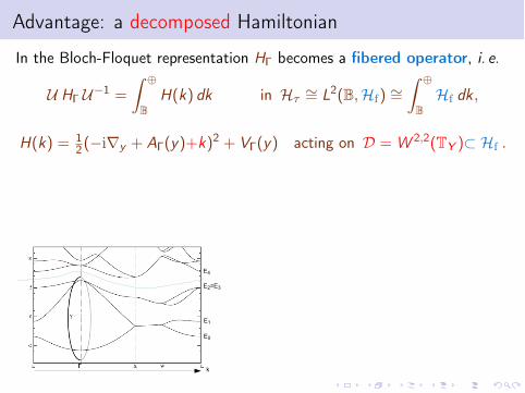
Advantage: a decomposed Hamiltonian
In the Bloch-Floquet representation H� becomes a fibered operator, i. e.
U H� U�1 =
Z �
BH(k) dk in H⌧
⇠= L2(B,Hf
) ⇠=Z �
BH
f
dk ,
H(k) = 1
2
(�iry
+ A�(y)+k)2 + V�(y) acting on D = W 2,2(TY
)⇢ Hf
.
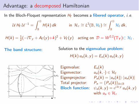
The band structure:
Solution to the eigenvalue problem:
H(k) un
(k , y) = En
(k) un
(k , y)
Eigenvalue: En
(k)Eigenvector: u
n
(k , ·) 2 Hf
Eigenprojector: Pn
(k) = |un
(k)i hun
(k)|Total projector: P
n
= {Pn
(k)}k2B
Bloch function: n
(k , y) = ei k·y un
(k , y)with u
n
2 H⌧
Advantage: a decomposed Hamiltonian
In the Bloch-Floquet representation H� becomes a fibered operator, i. e.
U H� U�1 =
Z �
BH(k) dk in H⌧
⇠= L2(B,Hf
) ⇠=Z �
BH
f
dk ,
H(k) = 1
2
(�iry
+ A�(y)+k)2 + V�(y) acting on D = W 2,2(TY
)⇢ Hf
.
The band structure:
Solution to the eigenvalue problem:
H(k) un
(k , y) = En
(k) un
(k , y)
Eigenvalue: En
(k)Eigenvector: u
n
(k , ·) 2 Hf
Eigenprojector: Pn
(k) = |un
(k)i hun
(k)|Total projector: P
n
= {Pn
(k)}k2B
Bloch function: n
(k , y) = ei k·y un
(k , y)with u
n
2 H⌧
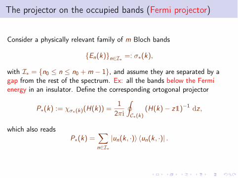
The projector on the occupied bands (Fermi projector)
Consider a physically relevant family of m Bloch bands
{En
(k)}n2I⇤ =: �⇤(k),
with I⇤ = {n0
n n0
+ m � 1}, and assume they are separated by agap from the rest of the spectrum. Ex: all the bands below the Fermienergy in an insulator. Define the corresponding ortogonal projector
P⇤(k) := ��⇤(k)(H(k)) =1
2⇡i
I
C⇤(k)(H(k)� z1)�1 dz ,
which also readsP⇤(k) =
X
n2I⇤|u
n
(k , ·)i hun
(k , ·)| .
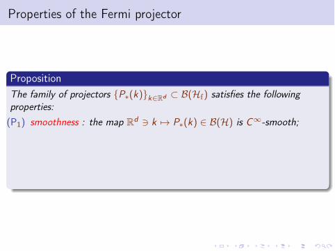
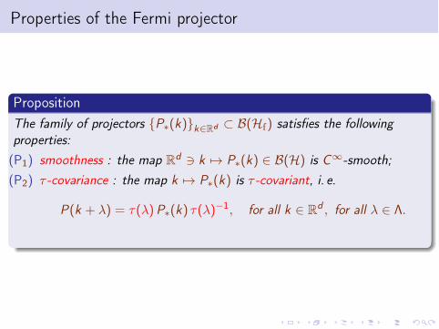
Properties of the Fermi projector
Proposition
The family of projectors {P⇤(k)}k2Rd ⇢ B(H
f
) satisfies the followingproperties:
(P1
) smoothness : the map Rd 3 k 7! P⇤(k) 2 B(H) is C1-smooth;(P
2
) ⌧ -covariance : the map k 7! P⇤(k) is ⌧ -covariant, i. e.
P(k + �) = ⌧(�)P⇤(k) ⌧(�)�1, for all k 2 Rd , for all � 2 ⇤.

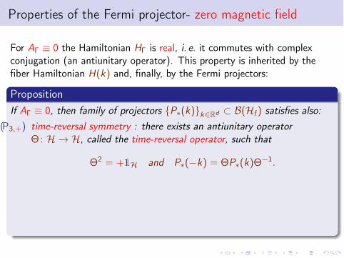
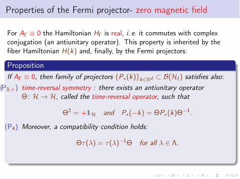
Properties of the Fermi projector- zero magnetic field
For A� ⌘ 0 the Hamiltonian H� is real, i. e. it commutes with complexconjugation (an antiunitary operator). This property is inherited by thefiber Hamiltonian H(k) and, finally, by the Fermi projectors:
Proposition
If A� ⌘ 0, then family of projectors {P⇤(k)}k2Rd ⇢ B(H
f
) satisfies also:(P
3,+) time-reversal symmetry : there exists an antiunitary operator⇥ : H ! H, called the time-reversal operator, such that
⇥2 = +1H and P⇤(�k) = ⇥P⇤(k)⇥�1.
(P4
) Moreover, a compatibility condition holds:
⇥⌧(�) = ⌧(�)�1⇥ for all � 2 ⇤.
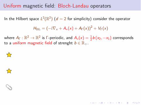
Uniform magnetic field: Bloch-Landau operators
In the Hilbert space L2(R2) (d = 2 for simplicity) consider the operator
HBL
= (�irx
+ A⇤(x) + A�(x))2 + V�(x)
where A� : R2 ! R2 is �-periodic, and A⇤(x) = 1
2
b (x2
,�x1
) correspondsto a uniform magnetic field of strenght b 2 R+.
Apparent breaking of translation invariance
The operator HBL
does not commute with the traslations {T�}�2�.
Recovery of translation invariance
Solution: use the magnetic translations T̃� introduced in [Zak].
References
[Zak] Zak, J.: Magnetic translation group, Phys. Review 134 (1964).
Uniform magnetic field: Bloch-Landau operators
Unfortunately, the magnetic translations do not commute among eachother. When considering � = SpanZ {e1
, e2
}, one has
T̃e1T̃e2 = ei�(b)/�?T̃
e2T̃e1
where �(b) = b(e1
^ e2
) is the magnetic flux per unit cell, and�? =
hc
e
⌘ 2⇡ is the fundamental unit of flux.
Rational flux, enlarged periodicity lattice
If �(b)/�? = 2⇡p/q 2 2⇡Q, one recovers periodicity with respect tothe lattice �
q
= SpanZ {e1
, qe2
}, since T̃e1T̃qe2 = T̃
qe2T̃e1 .
Uniform magnetic field: Bloch-Landau operators
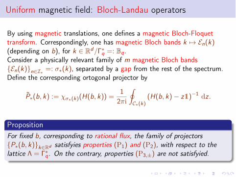
By using magnetic translations, one defines a magnetic Bloch-Floquettransform. Correspondingly, one has magnetic Bloch bands k 7! E
n
(k)(depending on b), for k 2 Rd/�⇤
q
=: Bq
.Consider a physically relevant family of m magnetic Bloch bands{E
n
(k)}n2I⇤ =: �⇤(k), separated by a gap from the rest of the spectrum.
Define the corresponding ortogonal projector by
P̃⇤(b, k) := ��⇤(k)(H(b, k)) =1
2⇡i
I
C⇤(k)(H(b, k)� z1)�1 dz .
Proposition
For fixed b, corresponding to rational flux, the family of projectors{P⇤(b, k)}
k2Rd satisfyies properties (P1
) and (P2
), with respect to thelattice ⇤ = �⇤
q
. On the contrary, properties (P3,±) are not satisfyied.
Uniform magnetic field: Bloch-Landau operators
By using magnetic translations, one defines a magnetic Bloch-Floquettransform. Correspondingly, one has magnetic Bloch bands k 7! E
n
(k)(depending on b), for k 2 Rd/�⇤
q
=: Bq
.Consider a physically relevant family of m magnetic Bloch bands{E
n
(k)}n2I⇤ =: �⇤(k), separated by a gap from the rest of the spectrum.
Define the corresponding ortogonal projector by
P̃⇤(b, k) := ��⇤(k)(H(b, k)) =1
2⇡i
I
C⇤(k)(H(b, k)� z1)�1 dz .
Proposition
For fixed b, corresponding to rational flux, the family of projectors{P⇤(b, k)}
k2Rd satisfyies properties (P1
) and (P2
), with respect to thelattice ⇤ = �⇤
q
. On the contrary, properties (P3,±) are not satisfyied.
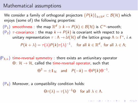
Mathematical assumptions
We consider a family of orthogonal projectors {P(k)}k2Rd ⇢ B(H) which
enjoys (some of) the following properties:(P
1
) smoothness : the map Rd 3 k 7! P(k) 2 B(H) is C1-smooth;(P
2
) ⌧ -covariance : the map k 7! P(k) is covariant with respect to aunitary representation ⌧ : ⇤ ! U(H) of the lattice group ⇤ ' �⇤, i. e.
P(k + �) = ⌧(�)P(k)⌧(�)�1, for all k 2 Rd , for all � 2 ⇤;
(P3,±) time-reversal symmetry : there exists an antiunitary operator
⇥ : H ! H, called the time-reversal operator, such that
⇥2 = ±1H and P(�k) = ⇥P(k)⇥�1.
(P4
) Moreover, a compatibility condition holds:
⇥⌧(�) = ⌧(�)�1⇥ for all � 2 ⇤.
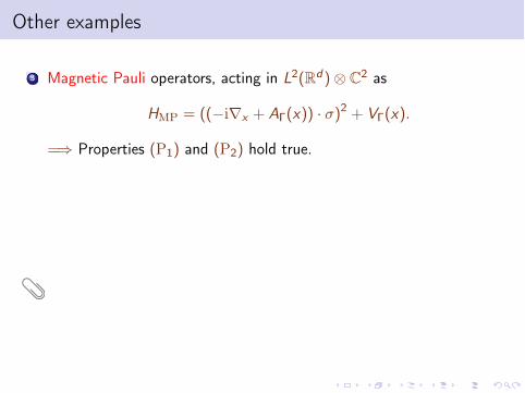
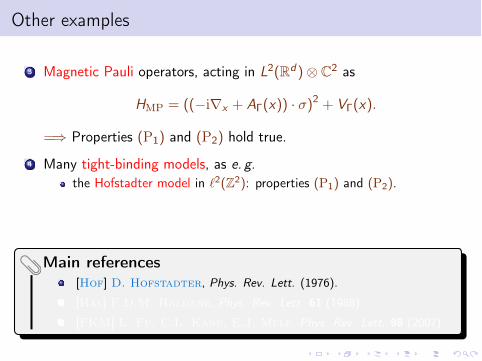
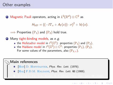
Other examples
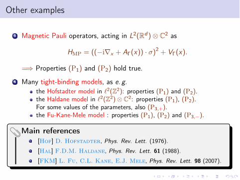
3 Magnetic Pauli operators, acting in L2(Rd )⌦ C2 as
HMP
= ((�irx
+ A�(x)) · �)2 + V�(x).
=) Properties (P1
) and (P2
) hold true.
4 Many tight-binding models, as e. g.the Hofstadter model in `2(Z2): properties (P1) and (P2).the Haldane model in `2(Z2)⌦ C2: properties (P1), (P2).For some values of the parameters, also (P3,+).the Fu-Kane-Mele model : properties (P1), (P2) and (P3,�).
Main references
[Hof] D. Hofstadter, Phys. Rev. Lett. (1976).
[Hal] F.D.M. Haldane, Phys. Rev. Lett. 61 (1988).
[FKM] L. Fu, C.L. Kane, E.J. Mele, Phys. Rev. Lett. 98 (2007).
Other examples
3 Magnetic Pauli operators, acting in L2(Rd )⌦ C2 as
HMP
= ((�irx
+ A�(x)) · �)2 + V�(x).
=) Properties (P1
) and (P2
) hold true.
4 Many tight-binding models, as e. g.the Hofstadter model in `2(Z2): properties (P1) and (P2).the Haldane model in `2(Z2)⌦ C2: properties (P1), (P2).For some values of the parameters, also (P3,+).the Fu-Kane-Mele model : properties (P1), (P2) and (P3,�).
Main references
[Hof] D. Hofstadter, Phys. Rev. Lett. (1976).
[Hal] F.D.M. Haldane, Phys. Rev. Lett. 61 (1988).
[FKM] L. Fu, C.L. Kane, E.J. Mele, Phys. Rev. Lett. 98 (2007).
Section 2
The Bloch bundle
and its Chern numbers
c� Animated pictures by Domenico Monaco
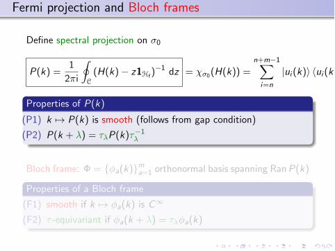
Fermi projection and Bloch frames
Define spectral projection on �0
P(k) =1
2⇡i
I
C
(H(k)� z1Hf
)�1 dz = ��0
(H(k)) =n+m�1X
i=n
|ui
(k)i hui
(k)|
Properties of P(k)
(P1) k 7! P(k) is smooth (follows from gap condition)
(P2) P(k + �) = ⌧�P(k)⌧�1
�
Bloch frame: � = {�a
(k)}ma=1
orthonormal basis spanning RanP(k)
Properties of a Bloch frame
(F1) smooth if k 7! �a
(k) is C1
(F2) ⌧ -equivariant if �a
(k + �) = ⌧��a
(k)
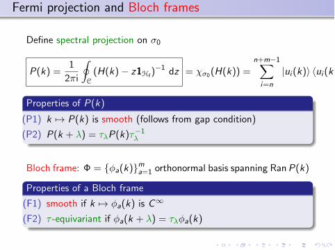
Wannier functions
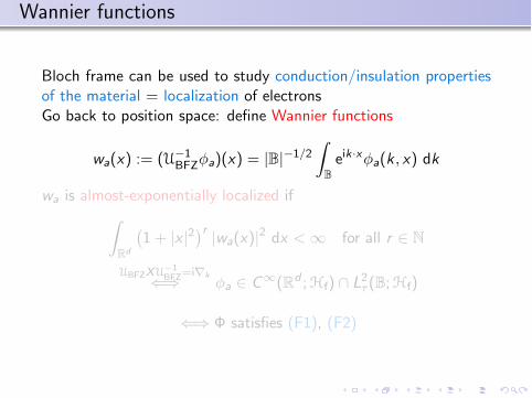
Bloch frame can be used to study conduction/insulation propertiesof the material = localization of electronsGo back to position space: define Wannier functions
wa
(x) := (U�1
BFZ
�a
)(x) = |B|�1/2Z
Beik·x�
a
(k , x) dk
wa
is almost-exponentially localized if
Z
Rd
�1 + |x |2
�r |w
a
(x)|2 dx < 1 for all r 2 N
UBFZ
XU�1
BFZ
=irk() �
a
2 C1(Rd ;Hf
) \ L2⌧ (B;Hf
)
() � satisfies (F1), (F2)
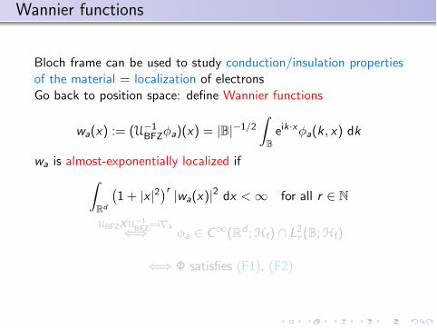
Wannier functions
Bloch frame can be used to study conduction/insulation propertiesof the material = localization of electronsGo back to position space: define Wannier functions
wa
(x) := (U�1
BFZ
�a
)(x) = |B|�1/2Z
Beik·x�
a
(k , x) dk
wa
is almost-exponentially localized if
Z
Rd
�1 + |x |2
�r |w
a
(x)|2 dx < 1 for all r 2 N
UBFZ
XU�1
BFZ
=irk() �
a
2 C1(Rd ;Hf
) \ L2⌧ (B;Hf
)
() � satisfies (F1), (F2)
Wannier functions
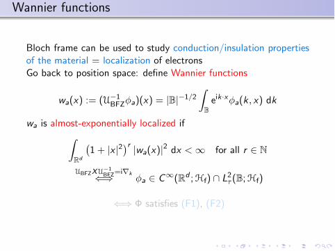
Bloch frame can be used to study conduction/insulation propertiesof the material = localization of electronsGo back to position space: define Wannier functions
wa
(x) := (U�1
BFZ
�a
)(x) = |B|�1/2Z
Beik·x�
a
(k , x) dk
wa
is almost-exponentially localized if
Z
Rd
�1 + |x |2
�r |w
a
(x)|2 dx < 1 for all r 2 N
UBFZ
XU�1
BFZ
=irk() �
a
2 C1(Rd ;Hf
) \ L2⌧ (B;Hf
)
() � satisfies (F1), (F2)
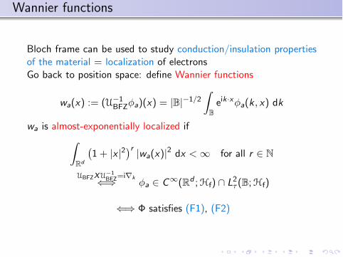
Wannier functions
Bloch frame can be used to study conduction/insulation propertiesof the material = localization of electronsGo back to position space: define Wannier functions
wa
(x) := (U�1
BFZ
�a
)(x) = |B|�1/2Z
Beik·x�
a
(k , x) dk
wa
is almost-exponentially localized if
Z
Rd
�1 + |x |2
�r |w
a
(x)|2 dx < 1 for all r 2 N
UBFZ
XU�1
BFZ
=irk() �
a
2 C1(Rd ;Hf
) \ L2⌧ (B;Hf
)
() � satisfies (F1), (F2)
Existence of a smooth, periodic Bloch frame
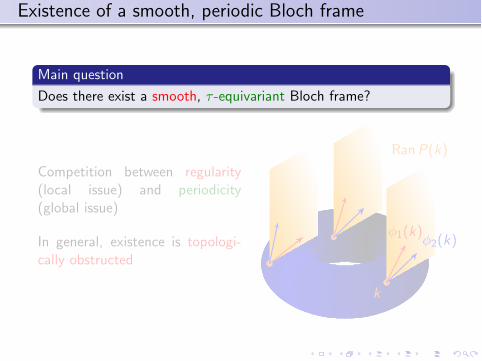
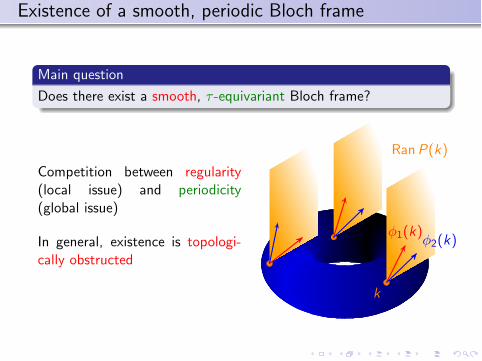
Main question
Does there exist a smooth, ⌧ -equivariant Bloch frame?
Competition between regularity(local issue) and periodicity(global issue)
In general, existence is topologi-cally obstructed
�1
(k)�2
(k)
k
RanP(k)
Existence of a smooth, periodic Bloch frame
Main question
Does there exist a smooth, ⌧ -equivariant Bloch frame?
Competition between regularity(local issue) and periodicity(global issue)
In general, existence is topologi-cally obstructed
�1
(k)�2
(k)
k
RanP(k)
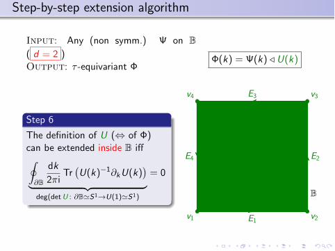
Step-by-step extension algorithm
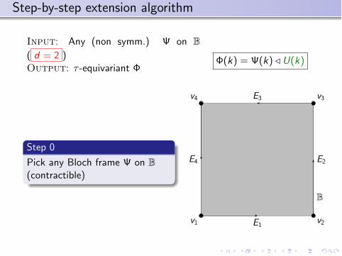
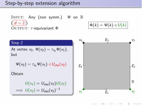
Input: Any (non symm.) on B( d = 2 )Output: ⌧ -equivariant �
�(k) = (k) / U(k)
Step 0
Pick any Bloch frame on B(contractible)
E1
E2
E3
E4
v1 v2
v3v4
B
Step-by-step extension algorithm
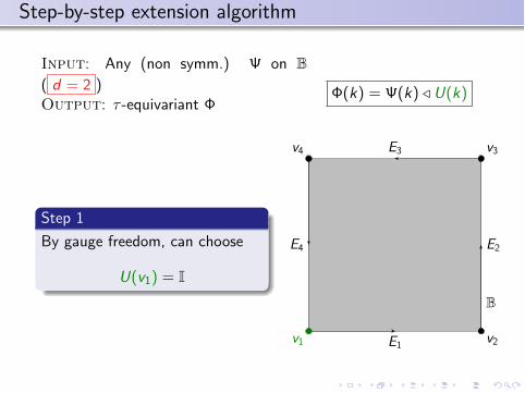
Input: Any (non symm.) on B( d = 2 )Output: ⌧ -equivariant �
�(k) = (k) / U(k)
Step 1
By gauge freedom, can choose
U(v1
) = I
E1
E2
E3
E4
v1 v2
v3v4
B
Step-by-step extension algorithm
Input: Any (non symm.) on B( d = 2 )Output: ⌧ -equivariant �
�(k) = (k) / U(k)
Step 2
At vertex v2
, �(v2
) = ⌧e
1
�(v1
),but
(v2
) = ⌧e
1
(v1
) / Uobs
(v2
)
Obtain
U(v1
) = Uobs
(v2
)U(v2
)
=) U(v2
) = Uobs
(v2
)�1
E1
E2
E3
E4
v1 v2
v3v4
B
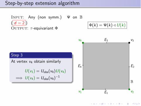
Step-by-step extension algorithm
Input: Any (non symm.) on B( d = 2 )Output: ⌧ -equivariant �
�(k) = (k) / U(k)
Step 3
At vertex v4
obtain similarly
U(v1
) = Uobs
(v4
)U(v4
)
=) U(v4
) = Uobs
(v4
)�1
E1
E2
E3
E4
v1 v2
v4 v3
B
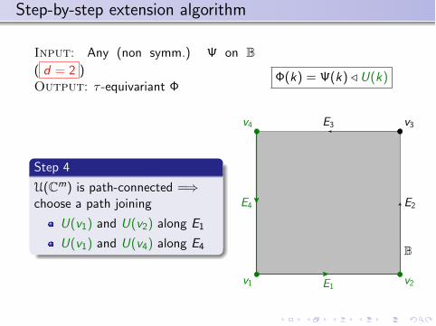
Step-by-step extension algorithm
Input: Any (non symm.) on B( d = 2 )Output: ⌧ -equivariant �
�(k) = (k) / U(k)
Step 4
U(Cm) is path-connected =)choose a path joining
U(v1
) and U(v2
) along E1
U(v1
) and U(v4
) along E4
E1
E2
E3
E4
v1 v2
v4 v3
B
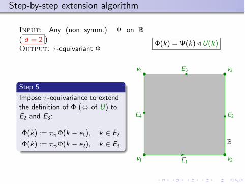
Step-by-step extension algorithm
Input: Any (non symm.) on B( d = 2 )Output: ⌧ -equivariant �
�(k) = (k) / U(k)
Step 5
Impose ⌧ -equivariance to extendthe definition of � (, of U) toE2
and E3
:
�(k) := ⌧e
1
�(k � e1
), k 2 E2
�(k) := ⌧e
2
�(k � e2
), k 2 E3
E1
E2
E3
E4
v1 v2
v3v4
B
Step-by-step extension algorithm
Input: Any (non symm.) on B( d = 2 )Output: ⌧ -equivariant �
�(k) = (k) / U(k)
Step 6
The definition of U (, of �)can be extended inside B i↵I
@B
dk
2⇡iTr
�U(k)�1@
k
U(k)�
| {z }deg(detU : @B'S
1!U(1)'S
1
)
= 0
E1
E2
E3
E4
v1 v2
v3v4
B
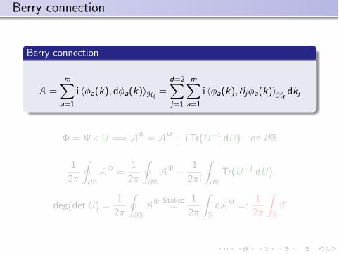
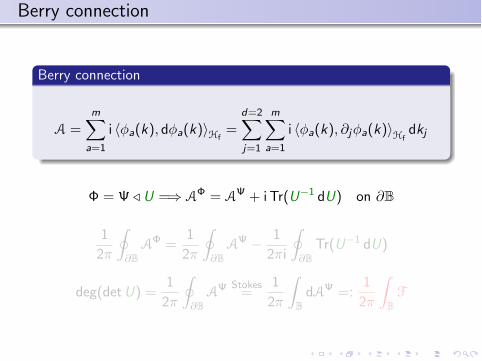
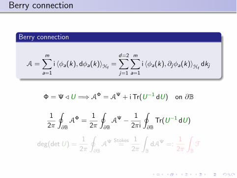
Berry connection
Berry connection
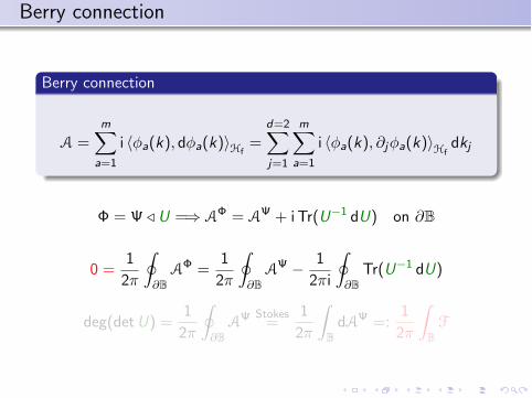
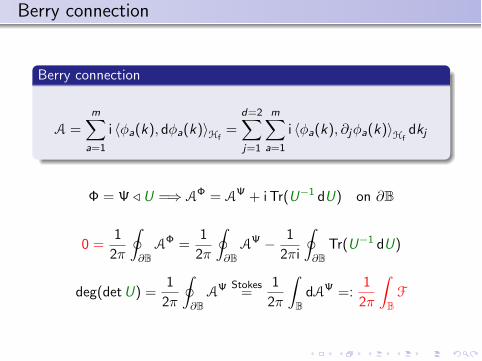
A =mX
a=1
i h�a
(k), d�a
(k)iHf
=d=2X
j=1
mX
a=1
i h�a
(k), @j
�a
(k)iH
f
dkj
� = / U =) A� = A + iTr(U�1 dU) on @B
1
2⇡
I
@BA� =
1
2⇡
I
@BA � 1
2⇡i
I
@BTr(U�1 dU)
deg(detU) =1
2⇡
I
@BA
Stokes
=1
2⇡
Z
BdA =:
1
2⇡
Z
BF
Berry connection
Berry connection
A =mX
a=1
i h�a
(k), d�a
(k)iHf
=d=2X
j=1
mX
a=1
i h�a
(k), @j
�a
(k)iH
f
dkj
� = / U =) A� = A + iTr(U�1 dU) on @B
1
2⇡
I
@BA� =
1
2⇡
I
@BA � 1
2⇡i
I
@BTr(U�1 dU)
deg(detU) =1
2⇡
I
@BA
Stokes
=1
2⇡
Z
BdA =:
1
2⇡
Z
BF
Berry connection
Berry connection
A =mX
a=1
i h�a
(k), d�a
(k)iHf
=d=2X
j=1
mX
a=1
i h�a
(k), @j
�a
(k)iH
f
dkj
� = / U =) A� = A + iTr(U�1 dU) on @B
1
2⇡
I
@BA� =
1
2⇡
I
@BA � 1
2⇡i
I
@BTr(U�1 dU)
deg(detU) =1
2⇡
I
@BA
Stokes
=1
2⇡
Z
BdA =:
1
2⇡
Z
BF
Berry connection
Berry connection
A =mX
a=1
i h�a
(k), d�a
(k)iHf
=d=2X
j=1
mX
a=1
i h�a
(k), @j
�a
(k)iH
f
dkj
� = / U =) A� = A + iTr(U�1 dU) on @B
0 =1
2⇡
I
@BA� =
1
2⇡
I
@BA � 1
2⇡i
I
@BTr(U�1 dU)
deg(detU) =1
2⇡
I
@BA
Stokes
=1
2⇡
Z
BdA =:
1
2⇡
Z
BF
Berry connection
Berry connection
A =mX
a=1
i h�a
(k), d�a
(k)iHf
=d=2X
j=1
mX
a=1
i h�a
(k), @j
�a
(k)iH
f
dkj
� = / U =) A� = A + iTr(U�1 dU) on @B
0 =1
2⇡
I
@BA� =
1
2⇡
I
@BA � 1
2⇡i
I
@BTr(U�1 dU)
deg(detU) =1
2⇡
I
@BA
Stokes
=1
2⇡
Z
BdA =:
1
2⇡
Z
BF
Berry curvature and Chern number
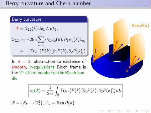
Berry curvature
F = F12
(k) dk1
^ dk2
,
F12
:= �2ImmX
a=1
h@1
a
(k), @2
a
(k)iHf
= �i TrHf
(P(k) [@1
P(k), @2
P(k)])
In d = 2, obstruction to existence ofsmooth, ⌧ -equivariant Bloch frame isthe 1st Chern number of the Bloch bun-dle
k
RanP(k)
c1
(P) =1
2⇡i
Z
BTrH
f
(P(k) [@1
P(k), @2
P(k)]) dk
P =�EP
! T2
⇤�, P
k
= RanP(k)
Section 2
The Bloch bundleand its Chern number