Embed Size (px)
Citation preview

COS429: COMPUTER VISON CAMERAS AND PROJECTIONS (2 lectures)
• Pinhole cameras•Analytical Euclidean geometry• The intrinsic parameters of a camera• The extrinsic parameters of a camera• Camera calibration• Least-squares techniques
Reading: Chapters 1 – 3, Forsyth & Ponce
Many of the slides in this lecture are courtesy to Prof. J. Ponce


Milestones:• Leonardo da Vinci (1452-1519): first record of camera obscura
Some history…

Milestones:• Leonardo da Vinci (1452-1519): first record of camera obscura• Johann Zahn (1685): first portable camera
Some history…
Photography (Niepce, “La Table Servie,” 1822)
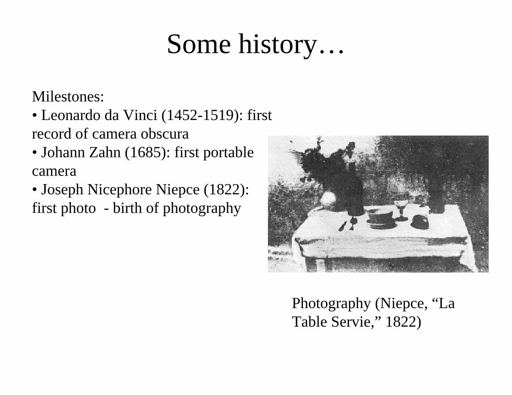
Milestones:• Leonardo da Vinci (1452-1519): first record of camera obscura• Johann Zahn (1685): first portable camera• Joseph Nicephore Niepce (1822): first photo - birth of photography
Some history…

Photography (Niepce, “La Table Servie,” 1822)
Milestones:• Leonardo da Vinci (1452-1519): first record of camera obscura• Johann Zahn (1685): first portable camera• Joseph Nicephore Niepce (1822): first photo - birth of photography• Daguerréotypes (1839)• Photographic Film (Eastman, 1889)• Cinema (Lumière Brothers, 1895)• Color Photography (LumièreBrothers, 1908)• Television (Baird, Farnsworth, Zworykin, 1920s)
Some history…

Let’s also not forget…
Motzu(468-376 BC)
Aristotle(384-322 BC)
Ibn al-Haitham(965-1040)

Pinhole perspective projection

Distant objects are smaller

Parallel lines meetCommon to draw image plane in front of the focal point. Moving the image plane merely scales the image.
Vanishing points
• Each set of parallel lines meets at a different point– The vanishing point for this direction
• Sets of parallel lines on the same plane lead to collinear vanishing points. – The line is called the horizon for that plane

Properties of Projection
• Points project to points• Lines project to lines• Planes project to the whole image or a half image • Angles are not preserved• Degenerate cases
– Line through focal point projects to a point.– Plane through focal point projects to line– Plane perpendicular to image plane projects to part of
the image (with horizon).

Pinhole Perspective Equation
⎪⎪⎩
⎪⎪⎨
⎧
=
=
zyfy
zxfx
''
''NOTE: z is always negative..

Affine projection models: Weak perspective projection
0
'where''
zfm
myymxx
−=⎩⎨⎧
−=−=
is the magnification.
When the scene depth is small compared its distance from theCamera, m can be taken constant: weak perspective projection.

Affine projection models: Orthographic projection
⎩⎨⎧
==
yyxx
'' When the camera is at a
(roughly constant) distancefrom the scene, take m=1.

Pros and Cons of These Models
• Weak perspective much simpler math.– Accurate when object is small and distant.– Most useful for recognition.
• Pinhole perspective much more accurate for scenes.– Used in structure from motion.
• When accuracy really matters, must model real cameras.

Diffraction effectsin pinhole cameras.
Shrinkingpinholesize
Use a lens!

Quantitative Measurements and Calibration
Euclidean Geometry

Euclidean Coordinate Systems
⎥⎥⎥
⎦
⎤
⎢⎢⎢
⎣
⎡=⇔++=⇔
⎪⎩
⎪⎨
⎧
===
zyx
zyxOPOPzOPyOPx
Pkjikji
...

Planes
⎥⎥⎥⎥
⎦
⎤
⎢⎢⎢⎢
⎣
⎡
=
⎥⎥⎥⎥
⎦
⎤
⎢⎢⎢⎢
⎣
⎡
−
=
=⇔=−++⇔=
1
and where
0.00.
zyx
dcba
dczbyaxAP
PΠ
PΠn

Coordinate Changes: Pure Translations
OBP = OBOA + OAP , BP = AP + BOA

Coordinate Changes: Pure Rotations
⎥⎥⎥
⎦
⎤
⎢⎢⎢
⎣
⎡=
BABABA
BABABA
BABABABA R
kkkjkijkjjjiikijii
.........
[ ]AB
AB
AB kji=

Coordinate Changes: Pure Rotations
⎥⎥⎥
⎦
⎤
⎢⎢⎢
⎣
⎡=
BABABA
BABABA
BABABABA R
kkkjkijkjjjiikijii
.........
⎥⎥⎥
⎦
⎤
⎢⎢⎢
⎣
⎡
=TB
A
TB
A
TB
A
kji

Coordinate Changes: Pure Rotations
[ ] [ ]
PRP
zyx
zyx
OP
ABA
B
B
B
B
BBBA
A
A
AAA
=⇒
⎥⎥⎥
⎦
⎤
⎢⎢⎢
⎣
⎡
=⎥⎥⎥
⎦
⎤
⎢⎢⎢
⎣
⎡
= kjikji

Coordinate Changes: Rotations about the z Axis
⎥⎥⎥
⎦
⎤
⎢⎢⎢
⎣
⎡−=
1000cossin0sincos
θθθθ
RBA

A rotation matrix is characterized by the following properties:
• Its inverse is equal to its transpose, and
• its determinant is equal to 1.
Or equivalently:
• Its rows (or columns) form a right-handedorthonormal coordinate system.

Coordinate Changes: Rigid Transformations
ABAB
AB OPRP +=

Block Matrix Multiplication
⎥⎦
⎤⎢⎣
⎡=⎥
⎦
⎤⎢⎣
⎡=
2221
1211
2221
1211
BBBB
BAAAA
A
What is AB ?
⎥⎦
⎤⎢⎣
⎡++++
=2222122121221121
2212121121121111
BABABABABABABABA
AB
Homogeneous Representation of Rigid Transformations
⎥⎦
⎤⎢⎣
⎡=⎥
⎦
⎤⎢⎣
⎡ +=⎥
⎦
⎤⎢⎣
⎡⎥⎦
⎤⎢⎣
⎡=⎥
⎦
⎤⎢⎣
⎡
11111P
TOPRPORP A
BA
ABAB
AA
TA
BBA
B
0

Rigid Transformations as Mappings

Rigid Transformations as Mappings: Rotation about the k Axis

Pinhole Perspective Equation
⎪⎪⎩
⎪⎪⎨
⎧
=
=
zyfy
zxfx
''
''

The Intrinsic Parameters of a Camera
Normalized ImageCoordinates
Physical Image Coordinates
Units:k,l : pixel/mf : mα,β : pixel

The Intrinsic Parameters of a Camera
Calibration Matrix
The PerspectiveProjection Equation

The Extrinsic Parameters of a Camera

Explicit Form of the Projection Matrix
Note:
M is only defined up to scale in this setting!!

Theorem (Faugeras, 1993)

Quantitative Measurements and the Calibration Problem

Calibration Procedure
• Calibration target : 2 planes at right angle with checkerboard (Tsai grid)
• We know positions of corners of grid with respect to a coordinate system of the target
• Obtain from images the corners• Using the equations (relating pixel coordinates to
world coordinates) we obtain the camera parameters (the internal parameters and the external (pose) as a side effect)

Estimation procedure
• First estimate M from corresponding image points and scene points (solving homogeneous equation)
• Second decompose M into internal and external parameters
• Use estimated parameters as starting point to solve calibration parameters non-linearly.

Homogeneous Linear Systems
A
A
x
x 0
0=
=
Square system:
• unique solution: 0
• unless Det(A)=0
Rectangular system ??
• 0 is always a solution
Minimize |Ax| under the constraint |x| =12
2

How do you solve overconstrained homogeneous linear equations ??
The solution is e .1
E(x)-E(e1) = xT(UTU)x-e1T(UTU)e1
= λ1μ12+ … +λqμq
2-λ1> λ1(μ1
2+ … +μq2-1)=0
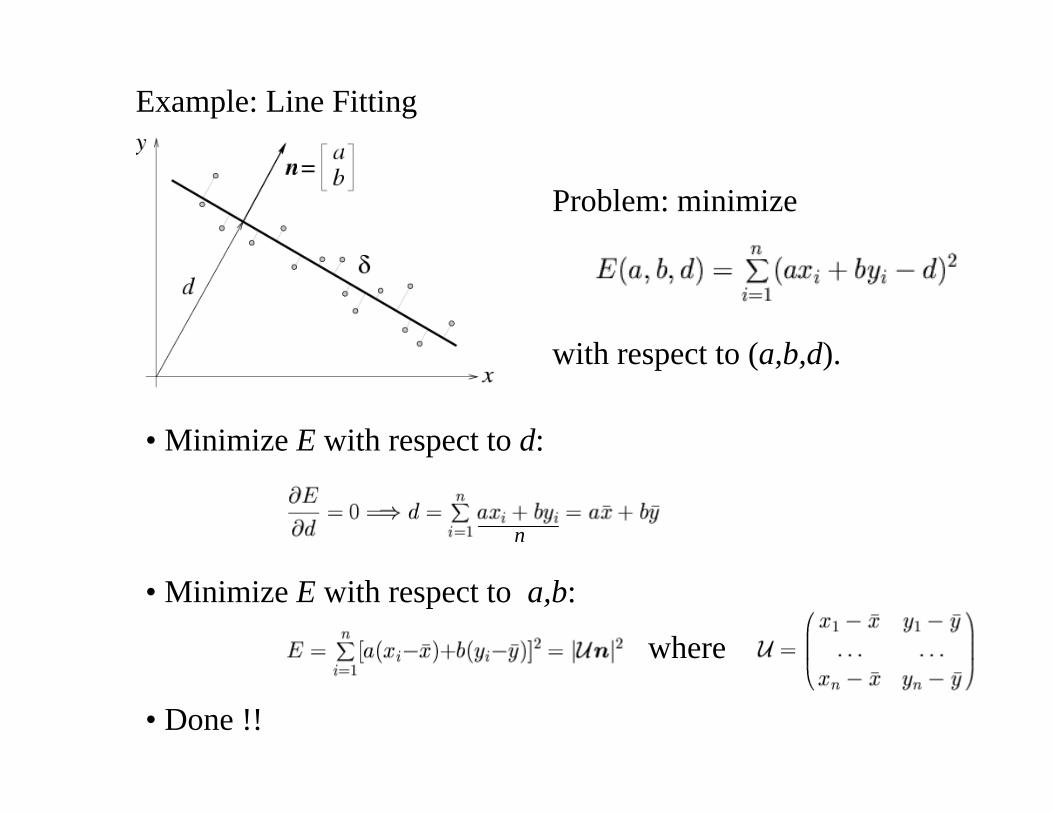
Example: Line Fitting
Problem: minimize
with respect to (a,b,d).
• Minimize E with respect to d:
• Minimize E with respect to a,b:
where
• Done !!
n

Note:
• Matrix of second moments of inertia
• Axis of least inertia

Linear Camera Calibration

Once M is known, you still got to recover the intrinsic andextrinsic parameters !!!
This is a decomposition problem, not an estimationproblem.
• Intrinsic parameters
• Extrinsic parameters
ρ

Degenerate Point Configurations
Are there other solutions besides M ??
• Coplanar points: (λ,μ,ν )=(Π,0,0) or (0,Π,0) or (0,0,Π )
• Points lying on the intersection curve of two quadricsurfaces = straight line + twisted cubic
Does not happen for 6 or more random points!

Analytical Photogrammetry
Non-Linear Least-Squares Methods
• Newton• Gauss-Newton• Levenberg-Marquardt
Iterative, quadratically convergent in favorable situations

Mobile Robot Localization (Devy et al., 1997)