Embed Size (px)
Citation preview
Lecture Based
Modules for Bridge Course in
Mathematics
All India Council for Technical Education Nelson Mandela Marg, Vasant Kunj, New Delhi 110 070
www.aicte-india.org
ALL INDIACOUNAL FAR TECI]NI'AL EOU'JlfIONL dute bosed Modules lot Bidae cou$es in ph$ics, Chenistto ond Mothendti..
PREFACE
Globalization of the world economy and higher education are driving profound changes incngincering education system. Worldwide adaptation of Outcome Based Education frameworkand enhanced focus on higher order learning and professional skills necessitates paradigm shiftin traditional practices ofcurriculum design, education delivery and assessment. AICTE has alsotaken various quality initiatives for strengthening the technical education system in lndia. Theseinitiatives are essential for promoting quality education in our institutions in the country so thatour students passing out from these institutions may match the pace with global standards.
A quality initiative by AICTE is 'Reyision of Curriculum'. Recently, AIC'I'E has released anoutcome based Model Curriculum for various Undergraduate degree courses in Engineering &Technology which are available on AlCl'E website. A thrce-week mandatory induction programis developed as a part of the model curriculum for the first year UG Engineering students whichhelps students ,oining the first year of the college from diverse backgrounds to get adjusted inthe new environment ofthe institution.
Education is primarily conceived by students as one simple remembering facts by rote.However, Science education also requires clear understanding ofscience concepts and a properlogical thinking or a constructive thinking by students. We all know that the students seekingadmission in an undergraduate degree engineering program have passed their 10+2 in sciencebut it was felt that a student joining an engineering program after 10+2 require rein[orccmentof fundamental science concepts i.e. basic science courses in physics, Chemistry andMathematics. 'l'o support the students, gain better understanding, AICTE decided to initiate thctask of development of bridge courses in Physics, Chemistry and Mathematics and it wasentrusted to IIT-BHU. These bridge courses aim to accelerate the students, knowledge in thesesubjects acquired at 10+2 level; and also bridge the gap between the school science syllabus andthe level needed to understand their applications to cngineering concepts, Therefore, it wasdecided that after completion of the 3-week mandatory induction programme introduced forthe first year UG engineering students, bridge course in basic physics, Chemistry andMathematics may be taken up by universities/institutions for the students for the remainingpart of thc semester. The concerned LJniversity/institution has a flexibility to adopt thescmodules on bridge courses by adiusting teaching hours accordingly.
'I'hc lecture based modules in Physics, Chemistry and N4athematics have been dcveloped by ateam of respective Course Coordinators from Indian Institute of l'echnology, Banaras IIinduUniversity. AICTE approved institutions may utilize these modules ,Lecture
Based Modules forBridge Courses - Physics, Chemistry and Mathemqtics,fot Leaching students to he]p bridge the gapoflhcir studies ol 10 i 2 and UG level.
(Prof. AnilChairman, AICTE
I . rD _;
budhc)

ALL INDA COUNCIL FOR TECHNICAL EOUCATIAN
Lat!rc bosed Madutes lot Bridge Caurset in phytics, AenEtty ond Mothenotit,
ACKNOWLEDGEMENT
Curriculum plays a crucial role in enabling quality learning for our young learners in our society
i.e. students. An effective curriculum not only enables a student's learning process & knowledge
acquired but also supports students to overcome their inhibitions and aids in their holisticdevelopment. AICTE in 2018 released a Model Curriculum for various Undergraduate degree
courses in Engineering & Technology. This curriculum is equipped with making students industry
ready, allow internships for hands on experience, learn about Constitution of lndaa, Environmentscience etc. lnduction program has been included as a mandatory program for the first year
engineering students to get acquainted and get accustomed to thas new environment in thecollege. a curriculum needs to be consistent and sustainable and it has been noticed that students
.joining an engineering program required to strengthen their concepts in science subjects i..e
Physics, Chemistry and Mathematics building a better foundation during the first semester itself.
AICTE therefore decided to develop lecture based bridge courses in basic science subjects i..e
Physics, Chemistry and Mathematics for students,. The lecture based modules in physics,
Chemistry and Mathematics have been developed by llT BHU. This task has been accomplishedby a team of respective Course Coordinators under Prof lndrajit Sinha, Department of Chemistry,llT BHU as Overall Coordinator.
AICTE places on record its acknowledgement and appreciation to Dr. lndrajit Sinha, Departmentof Chemistry, llT-BHU as overall coordinator; and respective course coordinators and their teamof facu ty members at llT-BHU for developing these lecture based modules for bridge courses:
The faculty team from llT BHU:
Depoftment of Pt tsics, ,tT, BHUProf. B. N. Dwivedi, Prof. O.N. Singh, Prof. D. Giri, Prof. p. Singh, prof. S. Chatterjee, prof. R. prasad, Dr.(N,4rs) A. Mohan, Dr. P.C. Pandey, Dr. (Mrs) 5. Upadhyay, Dr. A.K. Srivastava, Dr. S.K. l,4ishra, Dr. A.S.
Parmar, Dr. S. Tripathi, Dr. S. Patil, Dr. (Mrs) 5. N4ishra, Dr p. Dutta, Dr. S.K. Singh, Dr (Mrs) N. Agnihotri
Deportrnent of Chemastry, ,rl, BHU
Prof. R. B. Rastogi, Prof. A K Mukherjee, Prof. M A Quraishi, prof. V. Srivastava, prof. y.C. Sharma, prof. D.
Tiwari, Prof. K.D. Mandal, Dr. l. Sinha, Dr. S.Singh, Dr. M. Malviya
Depoftment of Mothemoticol Scien.es, tlT, BHLt
Prof. L. P. Singh, Prof. Rekha Srivastava, Prof. T Som, prof. S.K pandey prof. S.K. Upadhyay, prof. S. Das,Prof. S. Mukhopadhyay, Prof. S. Ram, prof. K.N. Rai, Dr. A.J. Gupta, Dr. Rajeev, Dr. R.K. pandey, Dr. V.K.
Singh, Dr. Sunil Kumar, Dr. Lavanya Shivkumar, Dr. A Beneiee, Dr. D. Ghosh, Dr. V.S. pandey
lnstitutions may adjust teaching hours to utilize these modules 'Lecture bosed Modutes for BridgeCourses Physics, Chemistry ond Mothemotics'to bridge the gap of 10+2 and UG level.
(Prof. Rajive Kumar)
Adviser-l(P&AP), AICTE
Mathematics Modules
(For AICTE Approved Colleges)
Prepared by
Department of Mathematical Sciences
Indian Institute of Technology
(Banaras Hindu University)
Varanasi - 221005

Contents
Module Lectures
1. Set Theory, Relations and Functions 03
2. Differential and Integral Calculus 02
3. Matrices and Determinants 02
4. Complex Numbers 03
5. Differential Equations 03
6. Analytical Geometry & Vector Algebra 03
7. Trigonometry 02
8. Probability 02
9. Statistics 02
Preface
The genesis of this module lies in the Induction Program first conceived and started by
IIT(BHU) on 2016 on mass scale for about 1000 students. The fact is that the students are
overburdened and stressed out due to a hectic high school life. To refresh their creative mind,
they were exposed to month long diverse credit courses like Physical Education, Human Values
and Creative Practices, as well as several non-credit informal activities. In a welcome step the
AICTE has proposed to extend this program to the Engineering Colleges affiliated to them.
Infact, purpose of this module is to bridge the gap between what the students need to know
before they can start taking the advanced courses in the college level and what they are actually
aware of from the intermediate level. Consequently, after the completion of the 3-weeks
induction program, it is proposed that (besides other subjects) bridge courses in basic Physics,
Chemistry and Mathematics should be taught to these students for the rest of the semester. The
bridge courses will cover typical weaknesses of students in science at the 10+2 level.
The modules in Mathematics are prepared keeping in mind that an hour of discussion will bring
all the students in the same stage such that they can cope up with the courses in their college
level, that requires the concepts of different topics in Mathematics. The modules are made as
interactive sessions between the students and the instructors. Furthermore, we have discussed
those topics which harder to understand. At the end of the discussion teacher may also take a
small test to understand how much the students followed the class.
In brief the contents of the modules are presented as follows. In Mudule-1, basic concepts of
sets, relations and function are discussed. Module -2 describes the definition of limit and
discuss some of its properties. After that we introduce the notion of continuity of a function
and the concept of the derivative of a function, and their properties.
Module-3, presents the idea of the basics of matrices, types of matrices, operations on matrices,
determinants and cofactors, computing inverse of a square matrix, rank and elementary
operations with brief discussion on system of linear equations.
Module-4 introduces the idea of the complex numbers and its basic properties. Further, the
definition of the complex sets, neighbourhood of a complex number, domain, complex
functions, limit of a complex functions and continuity of complex functions are presented in
detail with several examples.
Module-5 is devoted to the differential equations and includes the topics as the formation of
the differential equations, some special forms of the differential equations and then existence
and uniqueness of the first order differential equations. Module-6 focuses on the double and
triple integral and describes the method to solve such problems. It includes the other topics as
polar equations of conics, directional derivatives, gradients, divergence and curl. Module-7, 8
and 9 presents the basic idea of the trigonometry, probability and statistics respectively.
We are very much grateful to all the faculty members (Prof. L. P. Singh, Prof. Rekha
Srivastava, Prof. T. Som, Prof. S. K. Pandey, Prof. S. K. Upadhyay, Prof. S. Das, Prof. S.
Mukhopadhyay, Prof. S. Ram, Prof. K. N. Rai, Dr. A. J. Gupta, Dr. Rajeev, Dr. R. K. Pandey,
Dr. V. K. Singh, Dr. Sunil Kumar, Dr. Lavanya Shivkumar, Dr. A. Benerjee, Dr. D. Ghosh,

Dr. V. S. Pandey, in the Department of Mathematical Sciences who devoted their valuable time
to prepare these modules.
This is to mention that that modules are prepared for the students with an objective to create
interest among them in the subject. The references used in preparing these modules are cited at
end of each module.
Department of Mathematical Sciences,
IIT(BHU) Varanasi

Module-1: Set Theory, Relations and Functions
Module-1
Pretest on Sets, Relations and Functions
Sets
1) Specify the following sets in roster forms
(a) The set of prime numbers less than less than 20.
(b) The set of consonants in the word “VARANASI”.
2) Classify the following sets as finite, infinite, empty or singleton
(a) Even number which is prime.
(b) Set of teachers in your school.
(c) Cows which have five legs.
(d) The collection of integers.
3) Let , and be sets. Show that
i) ∪– ) ∪ii) ∩⊆
4) Let 0, 2, 4, 6, 8, 0, 1, 2, 4, 5, 6 and 4, 5, 6, 7, 8, 9, 10. Find
i) ∪∪ii) ∩∩
Relations
5) Let be a relation defined on , where 1, 2, 3, 4 such that , ) ∶ , , ∈. Write .
6) If 1, 2, 3 and 4, 5, 6, which of the following are relations from to
and why?
i) ! 1, 4), 1, 6), 2, 6)ii) " 2, 4), 2, 5), 3, 5), 3, 6), 3, 4)iii) # 4, 1), 1, 5), 2, 5)
7) In a set $ !, ", #, % of four men, ! is younger to other three, " is younger
to# and % only, # is younger to % only. Is the relation “is younger to” (i)
Reflexive, (ii) Symmetric and (iii) Transitive.
8) Find the domain and range of the relations defined on a set of real numbers :
i) For any two elements and of , iff 2 & 3 6.
ii) For , ∈, if and only if " & " 25.
Functions
9) Which of these are functions.

Module-1: Set Theory, Relations and Functions
2
10) Find the domain of the following function defined on set of real numbers:'() ))*!
11) Find the range of ' ∶ ℝ→ℝ where '() is given by (i) )*!),!, (ii) 3 − %
)*").,". 12) Is'() 4(#– 7, a bijective function?
13) If '() (" & 1, 0() (#, then find '10 and 01'.

Module-1: Set Theory, Relations and Functions
3
Module-1
Set Theory, Relations and Functions
Lectures required -02
In this module, we will discuss about the basic concepts of sets, relations and
function. The model is divided into three sections with three subsection each given below:
1. Set Theory
1.1 Definition and Representation
1.2 Types of Sets
1.3 Operation on Sets
2. Relations
2.1 Definition
2.2 Types of Relations
2.3 Partial order and Equivalence Relations
3. Functions
3.1 Definition and classification
3.2 Types of functions
3.3 Composition and Inverse of functions
1. Set Theory
A set is most basic term in mathematics. Hardly any discussion can proceed without sets
(class of collections). A set cannot be defined. Set is only primitive idea by which we can say
that such element belongs to the set or not.
A set is a collection of well defined distinct objects.
By “well-defined”, we mean “being unambiguous”, that is, when the idea assigns a
unique interpretation that given object in the world at large (abstract or concrete) is either an
element of set or it is not.
Notation: (∈2, is an element of 2.
Example: 1. The set of days in a week.
2. The set of integers i.e. ℤ . . . . . . . −3,−2, −1, 0, 1, 2, 3, . . . . . . . The following do not describe a well-defined collection and so are not sets.
Examples: 1. All good books.
2. The fruit which taste good to all.
1.1 Representations of sets: Sets can be represented by many ways. The most used are
(i) Roster form
(ii) Set-Builder form
(i) In the Roster form, the elements are enumerated as a list and are enclosed between
bracket “ ”
For example, 1, 2, 3, 4, 5. ℕ = Set of natural numbers = 1, 2, 3, . . . .
ℝ = Set of real numbers
Module-1: Set Theory, Relations and Functions
4
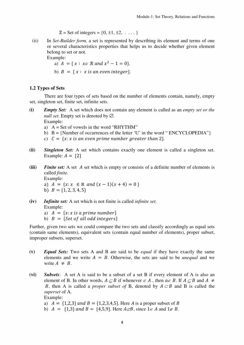
ℤ = Set of integers = 0, ±1, ±2, . . . .
(ii) In Set-Builder form, a set is represented by describing its element and terms of one
or several characteristics properties that helps us to decide whether given element
belong to set or not.
Example:
a) ( ∶ (∈ℛ6(" − 1 0. b) ( ∶ ( 666708.
1.2 Types of Sets
There are four types of sets based on the number of elements contain, namely, empty
set, singleton set, finite set, infinite sets.
(i) Empty Set: A set which does not contain any element is called as an empty set or the
null set. Empty set is denoted by ∅.
Example:
a) A = Set of vowels in the word “RHYTHM”
b) B = Number of occurrences of the letter ‘U’ in the word “ ENCYCLOPEDIA”
c) (:( 66:8;6<;808787ℎ62.
(ii) Singleton Set: A set which contains exactly one element is called a singleton set.
Example: 2
(iii) Finite set: A set set which is empty or consists of a definite number of elements is
called finite.
Example:
a) (:( ∈ ℝ6( − 1)( & 4) 0b) 1, 2, 3, 4, 5
(iv) Infinite set: A set which is not finite is called infinite set.
Example:
a) (: ( :8;6<;8 b) 271'AA16708
Further, given two sets we could compare the two sets and classify accordingly as equal sets
(contain same elements), equivalent sets (contain equal number of elements), proper subset,
improper subsets, superset.
(v) Equal Sets: Two sets A and B are said to be equal if they have exactly the same
elements and we write . Otherwise, the sets are said to be unequal and we
write ≠ .
(vi) Subsets: A set A is said to be a subset of a set B if every element of A is also an
element of B. In other words, ⊆ if whenever ∈ , then ∈. If ⊆ and ≠, then A is called a proper subset of B, denoted by ⊂ and B is called the
superset of A.
Example:
a) 1,2,36 1,2,3,4,5. Here is a proper subset of
b) 1,36 4,5,9. Here ⊄, since1∈ and 1∉.

Module-1: Set Theory, Relations and Functions
5
Apart from these, we have two more sets called the Power Set and Universal Set.
(vii) Power Set: A Power set of A is the set of all subsets of A and is denoted by P(A).
Example: If 1, 2, 3, then P) φ, 1, 2, 3, 1, 2, 1, 3, 2, 3, 1, 2, 3 If A has n-elements, then P (A) contains 2n elements.
(viii) Universal set : A set that contains all possible sets in a given context is called
universal set.
Example: C 1, 2, 3, 4, 5, 6, 7 when 1, 2, 3, 4 and 2, 3, 5, 6, 7 are subsets
of its universal set.
Venn diagrams: Sets and their relationships can also be represented by using diagrams,
called the Venn diagrams. Venn diagrams are graphic representation of sets as enclosed areas
in a plane region. This representation is named after the English Logician John Venn. In
Venn diagrams, the elements of the sets are written in their respective circles, while these sets
are encompassed in a rectangle by their Universal sets.
Example: A set A = 1,3,4,6,7,9,13,14 from its universal set U = 1, 2, … 15 can be
represented by
Note: A is contained in the universal set U.
3. Basic Operation on sets:
Given two sets A and B, there are various operations that can be performed namely,
then union or join, the intersection or meet, difference, symmetric difference and complement
of a set.
Here, except “complement”, all the other operations are binary operation, as we need
two sets to perform the operation. While the complement is an unary operation with reference
to the universal set. In addition, complements can also be viewed as binary operation of
difference C − ) between universal set and the set .
Historically, we could represent operation using Venn diagram as shown below :

Module-1: Set Theory, Relations and Functions
6
Operations Venn Diagram Representation
Partition of a set :
A partition of a set A is a collection of non-overlapping non-empty subsets of A
whose union is A.
(i.e.) If !, ", … , F⊆ then the collection δ = A1, ... An is called a partition, if
(i) G ≠φ, 1, 2, … , 6 (ii) G∩H φ, ≠I, , I 1, 2, . . 6, that is Ai’s are pairwise disjoint.
(iii) !∪". . .∪F (i.e.) ⋃ GFGK! .
For Example: A=1, 2, 3, 4, 5, 6, 7 , δ = 1, 4, 5, 2, 7, 3, 6, 8 is a partition of A.
Principle of inclusion-exclusion:
Let A and B be any two finite sets over a Universal set U, then n(A∪B) = n(A) + n(B) -
n(A∩B), where n(A) represents number of elements in the set A.
As to get number of elements of A∪B, we include number of elements of A and B,
and exclude (A∩B).
2. Relations
Let us consider two sets A and B: A = a1, a2, a3 and B= b1, b2, b3.
If one can indicate a relationship or association between (two or more objects) A and
B, then we can say there is a relation between A and B. Relations are given by subsets of the
cartesian product of sets ×. That is, let
!, !), !, "), !, #), ", !), ", "), ", #), #, !), #, "), #, #)
The complement of A:
A’=x∈∈∈∈U; x∉∉∉∉A
The symmetric difference:
A∆∆∆∆B= (A-B) ∩∩∩∩ (B-A)
The difference:
A-B=A\B=x: x∈∈∈∈A and x∉∉∉∉B
The intersection of A and B:
A∩∩∩∩B=x: x∈∈∈∈A and x∈∈∈∈B
The union of A and B:
A∪∪∪∪B=x: x∈∈∈∈A or x∈∈∈∈B
A
A B
A B
A B
A B

Module-1: Set Theory, Relations and Functions
7
Let R =(a1, b1), (a2, b3), (a3, b1) represents a relation between A and B.
Definition 1: Given two non-empty sets and , the relation from the set to set is
defined as the subset of ×.
If an ordered pair , )∈then we say 8A771). If ||=m and ||=n, then
|×|=mn. Then the number of relations on A and B are 2mn.
Domain and range of relations
Let be a relation from a set to set . Domain is the set consisting of all the first
elements of the ordered pairs belonging to and the range of the relation is the set of all
second element of the ordered pair of .
Therefore, Domain ) ∈ ∶ , )∈ and Range ) ∈ ∶ , )∈Example: A = 1, 2, 3 , B = a, b and R = (1, a), (2, b), (3, a), (3, b).
Domain for R = 1, 2, 3
Range of B = a, b
2.2 Types of relations :
i) Universal relation: If R = A×B, then R is called as universal relation.
ii) Null/Void/Empty Relation: If R=φ, then R is called empty.
iii) Inverse relation: If R is a relation from A to B, then R-1, inverse of R, is from B to S.
R-1 =(b,a) : (a,b)∈R.
Example: If 1, ), 1, M), 2, ), 2, )then *! , 1), M, 1), , 2), , 2)iv) Reflexive: If a relation R is such that aRa, ∀ ∈ , then R is said to reflexive
relation.
v) Irreflexive: If a relation R is such that aRa for every a∈R, that is, for every element a
in A, a is not related to itself.
vi) Non reflexive: If R is such that '18 1;∈, 6'18 1;∈, (that
is, for some element ∈, a is related to itself, while there are some ∈ not related to
itself. (vii) Symmetric relation: A relation R defined on set A is said to be symmetric
'⇒,Oℎ8, ∈. Example: For A = 1,2,3, R = (1,2), (2,1), (2,2), (1,3), (3,1)
R is symmetric, since 1,2)∈⇒2,1)∈ 2,2)∈⇒2,2)∈
1,3)∈⇒3,1)∈
(viii) Asymmetric Relation: P', )∈⇒, )∉, '18≠(ix) Antisymmetric Relation: A relation R is said to be antisymmetric,
', )∈, 6⇔ . In other words, if ≠ then either aRb or bRa or both.

Module-1: Set Theory, Relations and Functions
8
(x) Transitive Relation: A relation R on a set A is transitive if for
, , M∈, 6M7ℎ6M. Example: R = (1,2), (2,3), (1,3). Here, 1R2 and 2R3 ⇒ 1R3.
2.3 Partial Order and Equivalence Relations
A relation is said to be partially ordered if is reflexive, anti-symmetric and
transitive.
Example: R = (a,b) : a divides b, a,b ∉ ℕ.
(i) R is reflexive: Since a divides a ∀ ∈ ℕ.
(ii) R is antisymmetric:
aRb ⇒ a divides b
⇒ b=ak, k∈ ℕ
bRa ⇒ b divides a
⇒ a=bk,
⇒ b=ba1k
⇒ k1k1 =1.
⇒ k =1 and k1 =1.
⇒ a = b.
(iii) R is transitive :
Since aRb ⇒ a divides b ⇒ b = ak
bRc ⇒ b divides c ⇒ c = bk1
⇒ c = akk1 = ak2
⇒ a divides c
⇒ aRc.
∴ R is a partial order.
Equivalence relation:
A relation defined on is called an equivalence relation, if is reflexive,
symmetric and transitive.
Given a set A and an equivalence relation R, an equivalence class is subset of X of the form
[] (∈ ∶ (, Oℎ8∈[] - contains those elements which are equivalent to .
Set of all equivalence classes in A is called a Quotient set of A by R (A/R).
Set of all equivalence classes forms a partition of . Example: 1,2,3,4. 1,1, ), 2,2), 3,3), 4,4), 1,3), 2,4), 3,1), 4,2) is reflexive, symmetric and transitive. Hence, R is an equivalence relation.

Module-1: Set Theory, Relations and Functions
9
[1] 1,3 [3][2] 2,4 [4]
∴ [1] and [2] form the equivalence classes. Note that [1], [2] = 1,3, 2,4 forms a
partition of A.
3. Functions
Functions provide us a convenient way to handle a relationship between a variable
that depends on the value of another variable. Every function is a relation. However, every
relation does not become a function.
Definition : Let A and B be any two non-empty sets, then the rules or correspondence
between the elements of A and B is called a function from A to B if to each element of A,
there corresponds exactly one element of B. (i.e.) A function' ∶ →is a rule such that
every element of A has a unique image in B.
A is called the domain and B is called the co-domain.
Set of image of A (which is a subset of B) is called the range of f.
Example: A = 1,2, B = 1,3,4,5,6' ∶ → be defined as below:
Note f is a function.
Domain ') 1,2Range ') 1,5
Example 2: 1,2, 3,4, , , M, ,
Here f is not a function from A to B, since f(1) = a and
f(1) = c.
That is, 1 has no unique image.
Example. 3 : A = 1,2, 3,4,5, B = a, b, c, d
Here, f is not a function from A to B, since the
element 2∈A does not have an image in B.

Module-1: Set Theory, Relations and Functions
10
Note : (i) There may be elements in B not related to elements in A but every element of A
must have unique image in B.
(iii) If || ;and || 6, then the number of functions from A to B are nm.
Classification of functions
Functions are broadly classified into algebraic and transcendental functions.
Algebraic function represents polynomial functions and rational functions, while
transcendental functions are trigonometric functions, logarithmic and exponential functions.
3.2 Types of Functions
i) One to one function [Injective or Into]:
A function f : A →B is said to be one to one iff distinct elements of A have distinct
images in B (i.e.) x1, x2 ∈A, f(x1) = f(x2) ⇒ x1 = x2.
ii) Many to one functions :
A function from A to B is said to be many to one iff two or more elements of A have
same images in B.
Example: f(x) = x2, x ∈ ℝ
Suppose f(x1) = f(x2)
⇒ (!"= (""
⇒ x1 = ±x2
⇒ Every element of B has two pre-image in A.
f(1) = 12 = f(-1)
∴ f(x) is many to one function.
e.g. : Let f(x) = x2, x ∈ℝ+ [set of all positive reals].
Here, f is one-to-one
Suppose f(x1) = f(x2) ⇒ x1 = ±x2.
However x2 or- x2 does not belong to the domain of positive real numbers.
(iii) Onto functions
A mapping ':→is said to be onto if every element y ∈ B has some preimage x in
A, (i.e.) ∀y ∈ B x∈A such that f(x) =y.
Example: f(x) =2x-1, x ∈ℝ
Let y = f(x)
⇒ 2x-1 = y
⇒ x = S,!" ∈ℝ
(i.e.) x∈ R
f(x) = ' TS,!" U − 1 V

Module-1: Set Theory, Relations and Functions
11
(iv) Bijective Function
A function f : A to B is bijective, if f is one-to-one and onto.
' ∶ ℝ→ℝ, f(x) = 4x3 – 7.
One-One : f(x1) = f(x2) ⇒ 4(!# − V 4("# − V
⇒(!# − ("# 0
⇒(! − (")WT(! & )." U
" & #)..% X 0
⇒ x1 = x1 [(!" & (!(" & ("" > 0
Onto: V '() 4(# − 7⇒( TS,Z% U!/#, since y is real, for every y∈ℝ, there exists
an x∈ℝ such that f(x)=y.
∴ f is both one-one and onto and hence bijective.
3.3 Composition and Inverse of functions:
Composition of functions:
Let ': → and 0: → The composite of ' and 0 denoted by 01': → is defined by 01')() 0'()). Pictorially,
] 0V) 0^'()_ 01')() Similarly, for ': → , 0: →
'10: →
'10() '0()) Eg. 1,2,3, , , (, V ': → is '1) , '2) , '3)
0: → is 0) (, 0) V.

Module-1: Set Theory, Relations and Functions
12
01': → is defined as
01'1) 0^'1)_ 0) (
01'2) 0^'2)_ 0) (
01'3) 0^'3)_ 0) V.
Inverse of a function:
Let ': → and 0: → is called the inverse of ' if 01' P and '10 Pa where,
P : → defined by P ) is called the identity function on A.
That is, 0^'()_ (, ∀( ∈
and '^0V)_ V, ∀V ∈ .
The inverse of ' is also denoted by '*!.
Necessary and sufficient condition for inverse of ' to exists is that ': → is bijective, that
is, ' is one-one and onto.
Example: '() (% and 0() (!/%, ( ∈ ℝ
are inverses of each other.
'10)() '^0()_ ' T(bcU (!/%)% (
01')() 0^'()_ 0(%) (%)!/% (
Therefore, 01' Pℝ '10
i.e, ' and 0 are inverses of each other.
References:
1. P.B. Bhattacharya, S,.K.Jain, S.R. Nagpaul, First Course in Linear Algebra, Wiley,
1983.
2. G. Hadley, Linear Algebra, Narosa Publishing, 1992.
3. J.P. Singh, Discrete Mathematics for Under graduates, Ane Books, 2014.

Module-1: Set Theory, Relations and Functions
13
Assignment on Sets, Relations and Functions
Sets
1) Let A, B and C be sets. Shows the
i) – )– ⊆– ii) – )∩– )≠φ
2) Let 0, 2, 4, 6, 8, 0, 1, 2, 4, 5, 6 and 4, 5, 6, 7, 8, 9, 10. Find
i) A∪B)∩C ii) A∩B)∪C
3) Show that = A.
4) Let A a, b, c, B x, yandC 0, 1.Find
i) A×B×Cii) B×B×Biii) C×B×A
5) Which of these collections of subsets of partitions of 1, 2, 3, 4, 5, 6. i) 1, 2, 2, 3, 4, 4, 5, 6ii) 1, 2, 3, 6, 4, 5iii) 1, 4, 5, 2, 6
6) Give a formula for the number of elements in union of four sets.
7) How many positive integers not exceeding 1000 are divisible by 7 or 11?
Relations
8) Following relations are defined onA A, where A 1, 2, 3. Which of the
following relations are (i) Reflexive, (ii) Symmetric and (iii) Transitive.
i) R! 1, 1), 2, 3), 3, 3)ii) R" 1, 2), 2, 3), 2, 1)iii) R# 1, 2), 2, 3), 1, 3)iv) R% ∅
9) Give an example of a relation, which is
i) Reflexive but not symmetric
ii) Symmetric but not transitive
iii) Transitive but not reflexive.
10) Let R be a relation on the set of natural numbers such that , ) ∶ , , ∈p. Show that R is a partial order relation.
11) A relation R is defined on the setp p, where p is the set of natural numbers by
setting , )M, )⇔ & ) & M), , , M, ∈p. Show that this relation
is an equivalence relation.
12) If R is a relation on the set of an integer ℤ defined by , ) ∶ − 6'18, ∈ ℤ. Describe the equivalence classes of ℤ.

Module-1: Set Theory, Relations and Functions
14
13) Find the domain and range of the relations defined on a set of real numbers :
iii) For any two elements and of , iff 2 & 3 6.
iv) For , ∈, if and only if " & " 25.
Functions
14) Which of these are functions.
15) Find the domain of the following function defined on set of real numbers:
i) f(x) = !
)*|)|
ii) f(x) = !
qrsbt!*)) &√( & 2
16) If ' ∶ ℝ→ℝ be a function defined by f(x)= 2x2 + 3. Show that f(x) is not one to one
function.
17) If f(x)= x2 + 1, g(x) = x3, then find fog and gof.
18) If f(x)= log !*)!,), then prove that f(x) + f(y)= fT ),S
!*)SU.
19) Let ' ∶ ℝ→ℝ be defined by '() )√!,)., then show that
(i) '1'1')() )√!,#). and
(ii) '1'1')() ≠ ['()]#
20) If f(x) = v(" − 4( & 3,( w 26( − 4,( x 2
g(x) = v ( − 3,( w 3(" & 2( & 2,( x 3.
Determine f+g, f/g.
21) Let ' ∶ ℝ→ℝ and g ∶ ℝ→ℝ be two functions such that f(x) = 2x-3, g(x) = x3+5.
Then find (fog)-1(x).
22) Prove that' ∶ ℝ→ℝ defined by '() ) is one-one but not onto.

Module-2: Differential and Integral Calculus
Module-2
Pretest on Differential and Integral Calculus
Q. 1. If has a derivative at x=c, show that is continuous at x=c.
Q. 2. The function,
= 1, if is rational 0, if is irrational is discontinuous at …
Q. 3. The function
= 1, if ≠ 0 0, if = 0 is differentiable at x=0 or not? Give reason for your answer.
Q. 4. Evaluate
lim→ − log 1 + " #
Q. 5. If f(x) and g(x) are continuous for 10 ≤≤ x , could f(x) /g(x) possibly be discontinuous at a point of
[0, 1]? Give reason for your answer.
Q. 6. Give an example of function f and g, both continuous at x=0, for which the composite gf o is
discontinuous at x=0.
Q. 7. Suppose that h is integrable and . 6)( and 0)(
3
1-
1
1 ∫∫ ==−
drrhdrrh Find ∫ =
1
3
?)( drrh
Q. 8. For what values of c the following function
= $ " − 4 − 2 , if < 2 ; )" − ) − 8 , if ≥ 2 is continuous everywhere?
Q. 9. The expression ,- . ,- + . "- + ⋯ + .--# is a Riemann sum approximation for ……
(a)0 . - 1, (b) 0 √1, (c) ,- 0 . - 1, (d) ,- 0 √1, (e) ,- 0 √1-

Module-2: Differential and Integral Calculus
Module-2
Differential and Integral Calculus
Lectures required-02
A fundamental concept in single variable calculus is the concept of the limit of a function. In this
module, we first introduce the definition of limit and discuss some of its properties. After that we
introduce the notion of continuity of a function and the concept of the derivative of a function, and
their properties. Also we discuss some of the results related to continuity and differentiability. We
begin this module with some preliminary concepts.
Intervals: A subset ‘A’ of ℝ is called an interval if ‘A’ contains every element lies between any
two members of ‘A’.
i.e. whenever 4 ≤ ) ≤ 6 , where 4, 678
⟹ )78
Open Interval: 4, 6 = :7 ℝ/4 < < 6<
Neighbourhood of a point:
A set = ⊆ ℝ is called the neighbourhood of a point 47 ℝ, if there exists an open interval
I containing 4 and contained in =, i.e. 47? ⊆ =. Function:
Let 8 and A be two non-empty sets. 8 Function from 8 to A is a rule of correspondence
that assigns to each element in 8, a unique B in A.
8 is said to be the domain of and A, the co-domain of . Examples:
(1) The set ℝ of real numbers is the neighbourhood of each of its points. ∴ ∀ 7ℝ , ∃ an open interval − 7 , + 7), where s. t. 7 − 7 , + 7 ⊆ ℝ.
(2) ℕ, ℤ, H, HI are not the nbd of any of its points (since these sets do not contain any open
interval)
(3) J = K,L | 7ℕ N is not nbd of any real no.
Limit point of a Set: Let J ⊆ ℝ and O 7 ℝ then O is called a limit point of J if or any P > 0

Module-2: Differential and Integral Calculus
O − P, O + P ∩ J − :O< ≠ ∅
i.e. every nbd of O Contains at least one element of J other than O.
Note:
(1) A limit point of a set may or may not be a member of the set.
(2) O 7 ℝ is limit point of J ⊆ ℝ if every nbd of O contains infinite elements of J. Example: The set J = ℕNatural Number has no limit point.
∵ for any O 7 ℝ , any P > 0
(O − P, O + P) ∩ J if finite.
⟹ O is not a limit point ℕ
Here O is arbitrary ⇒ ℕ is no limit pt.
Example: The set K,L / 7ℕ N has only one limit point, zero, which is not a member of the set.
Limits
Limit of a function: Let be defined on an open interval about except possibly at itself.
We say that limit of as approaches is the number L if for every number 7 > 0, there
exist a corresponding number P > 0, s. t. for all ,
0 < | − | < P ⇒ | − Z| < [
OR:
Definition-2: Let 8 ⊆ ℝ, and let \ be a limit point of 8 for a function : 8 → ℝ, a real no. L is
said to be a limit of at \ if, given any 7 > 0 there exists a P > 0 such that if 7 8 and
0 < | − )| < P, then | − Z| < [.
Remarks:
(a): The inequality 0 < | − )| is equivalent to saying ≠ ). (b): Since the value of P usually depends on 7, we will sometimes write P7 instead of P. Question: Show that a function cannot have two different limits at the same point. That is, if lim→_ = Z, and lim→_ = Z" then Z, = Z".
Solution: Let, if possible, tend to limits Z, and Z" here for any > 0 , it is possible to choose
a P > 0 such that

Module-2: Differential and Integral Calculus
| − Z,| < " when 0 < | − | < P
| − Z"| < " when 0 < | − | < P
Now, |Z, − Z"| = |Z, − + − Z"| ≤ |Z, − | + | − Z"| < a" + a" = 7 when 0 < | − | < P
i.e. |Z, − Z"| is less than any positive number 7 (however small) and so must be equal to zero.
Thus Z, = Z" .
Question: Show that: lim→I = )" if = " , ≠ ) 1 , = ) b
Solution: We want to make the difference |" − )| less than a reassigned 7 > 0 by taking
sufficiently close to ). To do so, we note that
" − )" = + ) − ). Moreover, if | − )| < 1 then
|| < |)| + 1 , so that
| + )| ≤ || < |)| < 2|)| + 1. Therefore, if | − )| < 1, we have
|" − )| = | + )| ∙ | − )| < 2|)| + 1 ∙ | − )| (1)
Moreover this last term will be less than 7 provide we take | − )| < 7/2|)| + 1 Consequently, if we choose
P7: K1, a"|I|d, N
Then if 0 < | − )| < P7, it will follow first that | − )| < 1 so that (1) is valid, and therefore
since | − )| < 7/2|)| + 1 that |" − )"| < 2|)| + 1 ∙ | − )| < 7.
Since we have a way of choosing P7 for an arbitrary choice of 7 > 0, we infer that
= lim→I = )"
Exercise: Prove the limit statement lim→f" = 4 if = " , ≠ −2 1 , = −2 b

Module-2: Differential and Integral Calculus
Question: Let = 0 , if is rational 1, if is irrational b
Use definition of limit to prove that lim → does not exist.
Solution: Let Z 7ℝ Case-I: Z = 0
Let 7 = ,"
∀ P > 0, ∃ 7Hg Such that | − 0| < P (∵ Hg is dense in ℝ ) ∴ = 1
| − Z| = |1 − 0| = 1 ≥ ,"
∴ ∃ 7 > 0 , namely ," s.t. ∀ P > 0, ∃ s.t. | − 0| < P and | − 0| ≥ 7
∴ lim→ ≠ 0
Case-II: Z ≠ 0
Let 7 = |Z|/2 > 0
∀ P > 0, ∃ 7H such that | − 0| < P
∴ = 0
| − Z| = |0 − Z| = |Z| > |i|"
∴ ∃ 7 > 0, s.t ∀ P > 0, ∃ s.t. | − 0| < P and | − Z| ≥ 7
∴ lim→ ≠ Z
∄ Z7ℝ s.t. lim→ = Z
∴ lim→ does not exist.

Module-2: Differential and Integral Calculus
Continuity
Definition: Let 8 ⊆ ℝ, Let : 8 → ℝ, and let a 78. We say that is continuous at a if
lim→k = 4
In other words, the function is continuous at ‘4’, if for each 7 > 0, ∃ P > 0 s.t. | − 4| <7, when | − 4| < P. Discontinuous functions: A function is said to be discontinuous at a point ) of its domain if it is
not continuous there at. The point ) is then called a point of discontinuity of the function.
Types of discontinuities:
(i) A function is said to have a removable discontinuity at = ) if lim→I exists but is not
equal to the value ). (ii) is said to have a discontinuity of the first kind at = ) if lim→Il and lim→Im both
exist but are not equal.
(iii) is said to have a discontinuity of the second kind at = ) if neither lim→Il nor lim→Im exists.
Question: Suppose that is continous at and . Prove that there exists an open interval
containing on which > 0
Solution: Since is continuous at ,
lim→_ =
∴ for 7 = > 0, ∃ P > 0 s. t.
∴ | − | < P ⇒ | − | <
= − < < +
= > 0
∴ for 7 − P, + P, > 0.
Question: Show that if is continuous at = ), then so is ||. Is the converse true?
Solution: Let be continuous at = )
i.e. lim→I = )

Module-2: Differential and Integral Calculus
i.e. ∀ 7 > 0, ∃ P > 0 s.t.
| − | < P ⇒ | − )| < 7 ∀
⇒ n| − )|n < | − )| < 7
(by triangular inequality)
i.e. ∀ 7 > 0, ∃ P > 0 s.t.
| − | < P ⇒ n| − )|n < 7 ∀
i.e. lim→I|| = |)| ∴ || is continuous at = ). The Converse is not true.
i.e. || is continuous at = ) ⇏ is continuous at = )
e.g. Consider, = K 1, ≤ 2 −1, > 2 ∴ || = 1
|| is a constant function ⇒Continuous of = 2
But lim→" ≠ 2 = 1
∴ for 7 = 1 > 0
∀ P > 0, ∃ > 2 s. t. | − | < P
∵ | − 1| = |−1 − 1| = 2 > 7
∴ ∃ 7 > 0 s.t ∀ P > 0 ∃ s. t. | − | < P and | − 1| ≥ 7
∴ lim→" ≠ 1
So, is not continuous at = 2
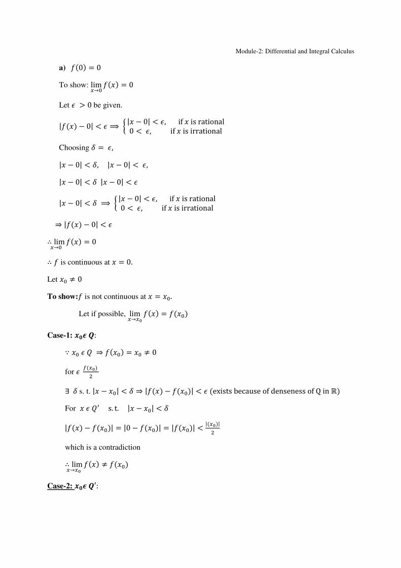
Question: Let = , if is rational 0, if is irrational a) Show that is continuous at = 0.
b) Show that is not continuous at every non-zero value of .
Solution:
Module-2: Differential and Integral Calculus
a) 0 = 0
To show: lim→ = 0
Let 7 > 0 be given.
| − 0| < 7 ⟹ | − 0| < 7, if is rational 0 < 7, if is irrational Choosing P = 7, | − 0| < P, | − 0| < 7, | − 0| < P | − 0| < 7 | − 0| < P ⟹ | − 0| < 7, if is rational 0 < 7, if is irrational
⇒ | − 0| < 7 ∴ lim→ = 0
∴ is continuous at = 0. Let ≠ 0
To show: is not continuous at = . Let if possible, lim→_ = Case-1: pqr s: ∵ 7 H ⇒ = ≠ 0 for 7 t_ "
∃ P s. t. | − | < P ⇒ | − | < 7 exists because of denseness of Q in ℝ
For 7 Hg s. t. | − | < P | − | = |0 − | = || < |_|"
which is a contradiction
∴ lim→_ ≠ Case-2: pqr s′:

Module-2: Differential and Integral Calculus
∴ = 0
for 7 = |_|" > 0
∃ P, s. t. | − | < P, ⇒ | − 0| < 7
Let P =min :P,, 7<
∴ | − | < P ⇒ | − Z| < 7
for 7 H s. t. | − | < P
| − 0| < |_|" ⇒ || < |_|" (i)
Further, n|| − ||n < | − | < P < 7
∴ n|| − ||n < |_|"
∴ || − |_|" < || < || + |_|"
∴ || > |_|" (ii)
by (i) & (ii), || < |_|" and || > |_|"
which is a contradiction.
∴ lim→_ ≠ ∴ is not continuous at ≠ 0
Intermediate Value Theorem: If a function is continuous on [4, 6] and 4 ≠ 6, then it
assumes every value between 4 and 6. Proof: Let 8 be any number between 4 & 6. We shall show that ∃ a number ) ∈ [4, 6] s.t. ) = 8. Consider a function ∅ defined on [4, 6] s.t.
∅ = − 8
clearly ∅ is continuous on [4, 6] . also, ∅4 = 4 − 8 41 ∅6 = 6 − 8 so that ∅4 and ∅6 are of opposite signs.( ∵ A lies between 4 & 6 )

Module-2: Differential and Integral Calculus
Thus the function ∅ is continuous on [4, 6] and ∅4 & ∅6 are of opposite signs therefore, ∃ ) 7 4, 6 s. t. ∅) = 0 ⇒ ) − 8 = 0 ⇒ ) = 8.
Differentiability
Definition: Let ? ⊆ ℝ be an interval, let : ? → ℝ, and let ) 7 ?. We say that a real number L is the
derivative of at ) if given any 7 > 0, ∃ P7 > 0
s.t. if 7 ? satisfies 0 < | − )| < P7, then
− ) − ) − Z < 7
In this case we say that is differentiable at ), and we write g) for L.
In other words, the derivative of at ) is given by the limit
g) = lim→I − ) − )
provided this limits exists.
Example: Show that the function = " is derivable on [0, 1]. Let be any point of 0, 1 then
g = lim→_" − " − = lim→_ + = 2exist finitely
at the end points, we have
g0 = lim→d tftf = lim→d = lim→d = 0 exist finitely
g1 = lim→,f tft,f, = lim→,f f,f, = lim→,f + 1 = 2 exist finitely
Thus the function is differentiable in [0, 1]. Example: A function is defined as:
= " J , , if ≠ 0 0, if = 0

Module-2: Differential and Integral Calculus
is derivable at = 0 but lim→ g ≠ g0
g0 = lim→ − 0 − 0 = lim→ " sin 1
= lim→ , = 0 ⇒ is differentiable at = 0. From elementary calculus, we know that for ≠ 0
g = 2 sin , − cos ,
Clearly, lim→g does not exist and therefore, there is no possibility of lim→g being equal to g0. Thus g is not continuous at = 0 but g0 exists.
Theorem: If : ? → ℝ has a derivative at ) 7 ?, then is continuous at ). Proof: for all 7 ?, ≠ ), we have
− ) = tftIfI − )
Since g) exists, so
lim→I − ) = lim→I − ) − ) # . lim→I − )
=g) × 0
Therefore, lim→I = ) so that is continuous at ).
Rolle’s Theorem: Suppose that is continuous on a closed interval ? = [4, 6], that the derivative ′ exists at every point of the open interval (a, b) and that 4 = 6. Then ∃ at least one point )
in (a, b) s. t. g) = 0. OR
If a function defined on [4, 6] is
(i) Continuous on [4, 6],

Module-2: Differential and Integral Calculus
(ii) derivable on 4, 6, and
(iii) 4 = 6
then ∃ at least one real no. ) between 4 & 6 4 < ) < 6 s. t. g) = 0
Proof: Do your-self.
Lagrange’s Mean Value Theorem:
If a function defined on [4, 6] is
(i) Continuous on [4, 6] and
(ii) derivable on (a, b),
then ∃ at least one real no. ) between 4 and 6 \ 7 4, 6 s.t.
g) = 6 − 46 − 4
Cauchy’s Mean Value Theorem:
If two functions , defined on [4, 6] are
(i) Continuous on [4, 6]
(ii) derivable on (a,b), and
(iii) g ≠ 0 , ∀ 7 4, 6
then ∃ at least one real no. ) between 4 & 6 s.t.
6 − 46 − 4 = g)g)
Theorem: Let : ? → ℝ be differentiable on the interval I. Then:
(a) is increasing on ? iff g ≥ 0 ∀ 7 ?
(b) is decreasing on ? iff g ≤ 0 ∀ 7 ?
Theorem: Let ? be on open interval and let : ? → ℝ have a second derivative on I. Then is a
convex function on ? iff gg ≥ 0 ∀ 7 ?

Module-2: Differential and Integral Calculus
Assignment
Q.1. Show that
a) Interval (Open/closed) is nbd of all of its members except the end points.
b) A non-empty finite set is not a nbd of any point.
c) Superset of a nbd of a point is also a nbd of .
d) If and = are nbds of a point , then that ∩ = is also a nbd of . Q.2. If a function is continuous on a closed interval [4, 6] and 4 & 6 are of opposite signs 4. 6 < 0, then there exists at least are point O 7 4, 6 s. t. O = 0.
Q.3. Show that the function defined by
= J 1 , when ≠ 0 0, when = 0 is continuous at = 0
Q.4. A function is defined on ℝ by
= −" ≤ 0 5 − 4 0 < ≤ 1 4" − 3 1 < < 2 3 + 4 ≥ 2
Examine for continuity at = 0, 1, 2. Also discuss the kind of discontinuity, if any.
Q.5. Is the function, where = f|| continuous?
Q.6. Show that = || + | − 1|, ∀ 7 ℝ
is continuous but not derivable at = 0 and = 1.
Q.7. Show that
= 1 , if ≠ 0 0, if = 0 is continuous but not derivable at the origin.
Q.8. Show that
= 0 , if ≤ 0 , if > 0

Module-2: Differential and Integral Calculus
is continuous but not derivable at = 0. Q.9. Show that for any real no. , the polynomial = + + has exactly one real root.
Q.10. Verify Rolle’s theorem for the function = − 9. Q.11. Use Intermediate value theorem to show that there is a root of = " − in the interval
(1, 2).
References:
• G.B. Thomas, M.D. Weir, J.R. Hass, Thomas’ Calculus, Pearson Publication.
• R.G. Bartle, D.R. Sherbert, Introduction to Real Analysis, Wiley Publication.

Module-2: Differential and Integral Calculus
Riemann Integrals
The Riemann integral, as it is called today, is the one fundamental topic usually discussed in
introductory calculus. In this module, we introduce the concept of Riemann integrals and
discuss some of its properties. Throughout this module, it is assumed that we are working with
a bounded function on a closed interval [4, 6].
Partition of [, ]: Let [4, 6] be a closed interval and let ,, … … … L are the points
of [4, 6] s.t.
4 = < , < …………………Lf, < L = 6
The define a set
= :4 = , , ", … … … … … … f,, … … … … … … . , L = 6<
is called a partition of [4, 6] with + 1 points; and ? = [f, , ] be the sub-
interval of [4, 6] obtained by the points f, & of . i. e.
?, = [, ,], ?" = [,, "], …………, ?¡ [f, , ], … … … … , ?L = [Lf, , L ] Length of ¢£¤ interval: = ¥ ? = |?| = | − f,| Norm of Partition: Let P be a partition of [4, 6] and ? = [f, , ], be the sub-
interval and ?? = ∆ = | − 1, | The norm of is denoted by § or‖‖ and defined as:
‖‖ = 4 :∆© | = 1 ª« <
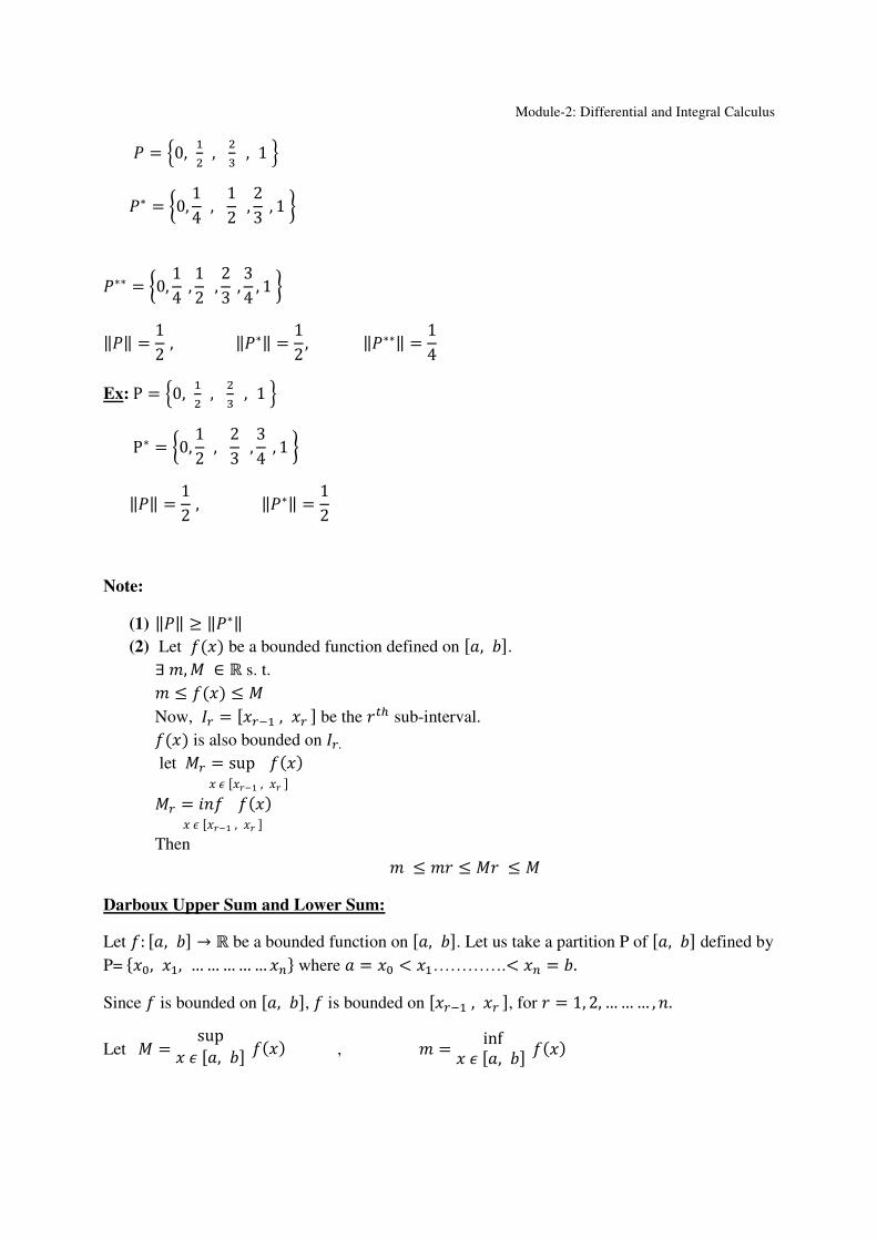
. . ? = [0, 1] Let = :0 = , ,, ", = 1<
= K0, ," , " , 1 N
?, = ¬0, ," , ?" = ¬," , " , ? = ¬" , 1
¥ ?, = ," , ¥ ?" = ,®, ¥ ? = ¯1 − "¯ = ,
So ‖‖ = max K ," , ,® , ,N = ,"
Refinement of Partition: Let and ∗ are two partitions of [4, 6] s. t. ⊆ ∗ then ∗ is
called the refinement or finer than .
Module-2: Differential and Integral Calculus
= K0, ," , " , 1 N
∗ = 0, 14 , 12 , 23 , 1 b
∗∗ = 0, 14 , 12 , 23 , 34 , 1 b
‖‖ = 12 , ‖∗‖ = 12, ‖∗∗‖ = 14 Ex: P = K0, ," , " , 1 N
P∗ = 0, 12 , 23 , 34 , 1 b
‖‖ = 12 , ‖∗‖ = 12
Note:
(1) ‖‖ ≥ ‖∗‖
(2) Let be a bounded function defined on [4, 6]. ∃ ², ∈ ℝ s. t. ² ≤ ≤
Now, ? = [f, , ] be the sub-interval. is also bounded on ?. let = sup
7 [f, , ] = 7 [f, , ] Then ² ≤ ² ≤ ≤
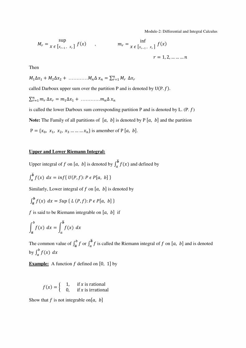
Darboux Upper Sum and Lower Sum:
Let : [4, 6] → ℝ be a bounded function on [4, 6]. Let us take a partition P of [4, 6] defined by
P= :, ,, … … … … … L< where 4 = < ,………….< L = 6. Since is bounded on [4, 6], is bounded on [f, , ], for = 1, 2, … … … , . Let = sup 7 [4, 6] , ² = inf 7 [4, 6]
Module-2: Differential and Integral Calculus
= sup 7 [−1 , ] , ² = inf 7 [−1 , ]
= 1, 2, … … …
Then
,∆, + "∆" + …………L∆ L = ∑ L¡, ∆
called Darboux upper sum over the partition P and is denoted by UP. . ∑ ²L¡, ∆ = ²,∆, + …………²L∆ L
is called the lower Darboux sum corresponding partition P and is denoted by L. (P. )
Note: The Family of all partitions of [4, 6] is denoted by P [4, 6] and the partition
P = :, ,, ", … … … L< is amember of P [4, 6].
Upper and Lower Riemann Integral:
Upper integral of on [4, 6] is denoted by 0 µk and defined by
0 µk 1 = : ¶, : 7 [4, 6] <
Similarly, Lower integral of on [4, 6] is denoted by
0 µ 1 = J·¸ : Z , : 7 [4, 6] <
is said to be Riemann integrable on [4, 6] if
¹ ºµ 1 = ¹ µ
k 1
The common value of 0 ºµ or 0 µk is called the Riemann integral of on [4, 6] and is denoted
by 0 ºk 1
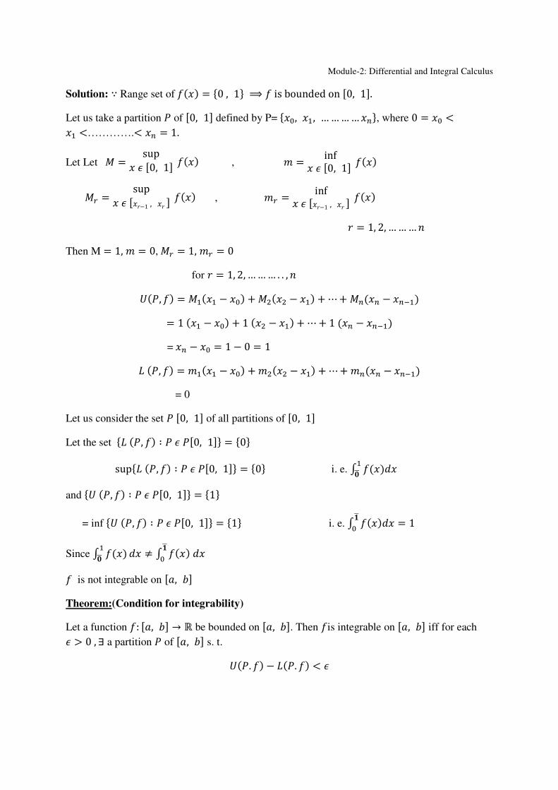
Example: A function defined on [0, 1] by
= 1, if is rational 0, if is irrational Show that is not integrable on[4, 6]
Module-2: Differential and Integral Calculus
Solution: ∵ Range set of = :0 , 1< ⟹ is bounded on [0, 1]. Let us take a partition of [0, 1] defined by P= :, ,, … … … … L<, where 0 = <, <………….< L = 1. Let Let = sup 7 [0, 1] , ² = inf 7 [0, 1]
= sup 7 [−1 , ] , ² = inf 7 [−1 , ]
= 1, 2, … … …
Then M = 1, ² = 0, = 1, ² = 0
for = 1, 2, … … … . . ,
¶, = ,, − + "" − , + ⋯ + LL − Lf,
= 1 , − + 1 " − , + ⋯ + 1 L − Lf,
= L − = 1 − 0 = 1
Z , = ²,, − + ²"" − , + ⋯ + ²LL − Lf,
= 0
Let us consider the set [0, 1] of all partitions of [0, 1] Let the set :Z , ∶ 7 [0, 1]< = :0<
sup:Z , ∶ 7 [0, 1]< = :0< i. e. 0 1,qµ
and :¶ , ∶ 7 [0, 1]< = :1<
= inf :¶ , ∶ 7 [0, 1]< = :1< i. e. 0 1 = 1¼µ
Since 0 ,qµ 1 ≠ 0 1¼µ
is not integrable on [4, 6] Theorem:(Condition for integrability)
Let a function : [4, 6] → ℝ be bounded on [4, 6]. Then is integrable on [4, 6] iff for each 7 > 0 , ∃ a partition of [4, 6] s. t.
¶. − Z. < 7
Module-2: Differential and Integral Calculus
Proof: Do yourself.
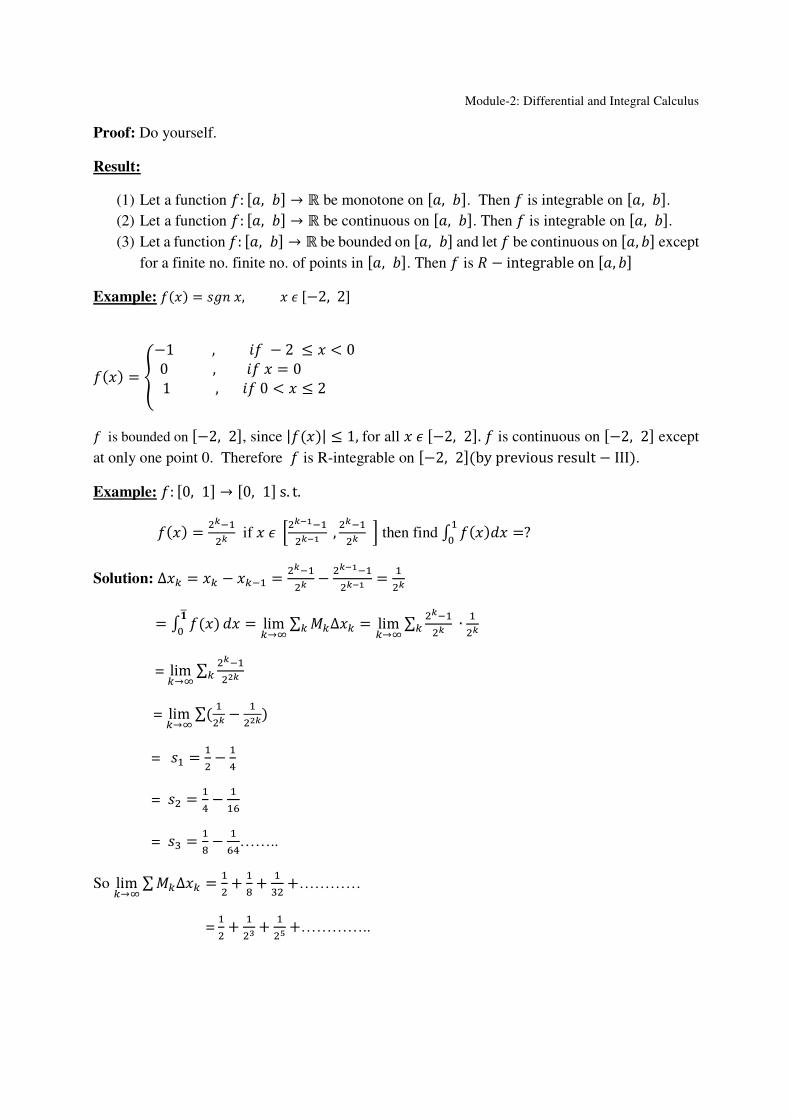
Result:
(1) Let a function : [4, 6] → ℝ be monotone on [4, 6]. Then is integrable on [4, 6]. (2) Let a function : [4, 6] → ℝ be continuous on [4, 6]. Then is integrable on [4, 6]. (3) Let a function : [4, 6] → ℝ be bounded on [4, 6] and let be continuous on [4, 6] except
for a finite no. finite no. of points in [4, 6]. Then is ½ − integrable on [4, 6] Example: = , 7 [−2, 2] = ¾−1 , − 2 ≤ < 0 0 , = 0 1 , 0 < ≤ 2
is bounded on [−2, 2], since || ≤ 1, for all 7 [−2, 2]. is continuous on [−2, 2] except
at only one point 0. Therefore is R-integrable on [−2, 2]by previous result − III.
Example: : [0, 1] → [0, 1] s. t. = "Áf,"Á if 7 ¬"Álf,"Ál , "Áf,"Á then find 0 1 =?,
Solution: ∆à = à − Ãf, = "Áf,"Á − "Álf,"Ál = ,"Á
= 0 ¼µ 1 = limÃ→Ä ∑ Ã∆Ãà = limÃ→Ä ∑ "Áf,"Áà ∙ ,"Á
= limÃ→Ä ∑ "Áf,"ÁÃ
= limÃ→Ä ∑ ,"Á − ,"Á
= , = ," − ,Å
= " = ,Å − ,,®
= = ,Æ − ,®Å……..
So limÃ→Ä ∑ Ã∆à = ," + ,Æ + ," +…………
= ," + ,"Ç + ,"È +…………..

Module-2: Differential and Integral Calculus
=
,fÉ = ," × Å = "
¹ ¼µ 1 = 23
Similarly, 0 ¼qµ 1 = "
So, 0 ¼ 1 = " .
Assignment
Q.1. Show that
a) ¶ , ≥ Z ,
b) ¶ , ≥ ¶ ∗,
c) Z , ≤ Z ∗,
d) ¶, ≥ Z ∗,
e) ¶ ∗, ≥ Z ∗, ≥ Z ,
Q.2. Discuss Riemann integrability of function
= [] , 7 [0, 2]. Q.3. Let: [0, 1] → R is the function = ". For any ε >0, choose a partition
= :0 = , , ", … … … … … … f,, … … … … … … . , L = 1<
such that © − ©f, < ε/2 for all 1 ≤ i ≤ n.
Show that ¶. − Z. < 7
Hence, is Reimann integrable.
References:
• G.B. Thomas, M.D. Weir, J.R. Hass, Thomas’ Calculus, Pearson Publication.
• R.G. Bartle, D.R. Sherbert, Introduction to Real Analysis, Wiley Publication.

Module-3: Matrices and Determinants
Module-3
Pretest on Matrices and Determinant
1) Find 3 − 2, if = 2 −1 04 7 15 3 2 and = −6 0 21 5 38 2 1
2) Find ( + ), if = 1 0 23 −5 70 0 3, = 3 56 20 2 and = 0 −83 110 4
3) Classify the type of matrix :
i) 1 3 53 4 −75 −7 6 , ii) 0 −4 −54 0 −75 7 0 , iii) 4 2 60 5 −30 0 1 ,
iv) 2 0 00 0 00 0 5, v) 1 00 1 4) Determine the matrices X & Y from the equation:
X + Y = 1 −23 4 , X - Y = 3 2−1 0 5) If = −1 23 1 , = 1 −13 4−1 5 does AB exists?
6) If A and B are two square matrices of same order. Is ( + ) = + 2 +
7) Apply the properties of determinants and calculate :
i) A= 1 2 34 5 67 8 9, ii) B= 1 0 10 1 00 0 1, and iii) C = 2 3 42 + 3 + 42 ! + 3 " + 4.

Module-3: Matrices and Determinants
2
Module-3
Matrices and Determinants
Lectures required -02
In this module, we discuss about the basics of matrices, types of matrices, operations
on matrices, determinants and cofactors, computing inverse of a square matrix, rank and
elementary operations with brief discussion on system of linear equations.
1. Matrices and Determinants
1.1 Types of Matrices
1.2 Operations on Matrices
1.3 Determinants and Cofactors
1.4 Inverse of a Square Matrix
1.5 Rank of Matrix
1.6 Elementary row / column operations
1.7 System of Linear Equations
1. Matrices and Determinants:
A matrix is defined to be a rectangular array of a number assigned into rows and
columns. A set of “mn” elements arranged in rectangular formation containing m-rows and n-
columns is called m×n matrix
A=
#$$$$%
&& & … &(& … (. . … .. . … .. . … .*& * … *(+,,,,-, where ./ are elements of the matrix A.
1.1 Type of Matrices :
There are around 12 types of matrix.
i) Row matrix : When m=1, the matrix with one row is called row matrix or
vector.
ii) Column matrix : When there is only one column i.e. n=1, the matrix is called
a column matrix.
iii) Square matrix : When m=n, that is number of rows is equal to number of
columns.
iv) Triangular Matrix : In a square matrix, when the elements above the
principal diagonal or below the principal diagonal are all zero, the matrix is
called triangular matrix.
v) Diagonal Matrix : In a square matrix, when the elements above and below the
principal diagonal is zero i.e. matrix is filled with zero elements except on the
main diagonal

Module-3: Matrices and Determinants
3
e.g. 2 0 00 −1 00 0 3
vi) Scalar matrix : Scalar matrix is a diagonal matrix in which all the elements
along the main diagonal are equal.
e.g. 2 0 00 2 00 0 2
vii) Unit matrix (Identity Matrix) : A scalar matrix with all the elements on the
diagonal are equal to 1.
e.g. 1 00 1 1 0 00 1 00 0 1
viii) Null or Zero Matrix : If all the elements in matrix are zero, then it is called
zero matrix
e.g. 0 0 00 0 0
ix) Symmetric matrix : A square matrix A = (aij) is called symmetric matrix if
aij= aji for all i and j.
e.g. 2 3 53 6 −75 −7 4
x) Skew symmetric matrix : A square matrix A = (aij) is called a skew
symmetric if aij= -aji for all i and j, i≠j and aii= 0 for all i.
e.g. 0 4 7−4 0 −5−7 5 0
xi) Singular matrix : If ||=0 (det(A)), then the matrix A is called singular.
xii) Non-singular matrix : If || ≠0, then the matrix A is called non-singular.
1.2 Operations on Matrices
(i) Addition of two matrices:
Addition of two matricesA=[aij]m×nand B=[bij]m×n can be defined only when both A
and B have same more same order.
= 2!./3*×( (= + ), 5ℎ787 !./ = ./ + ./, 1≤ 9 ≤ :, 1≤ ; ≤ < is the sum of A and B.
Example: A = 2 1 5−1 6 2, B = 0 5 −23 4 1
C = A + B = 2 + 0 1 + 5 5 − 2−1 + 3 6 + 4 2 + 1 = 2 6 32 10 3
Module-3: Matrices and Determinants
4
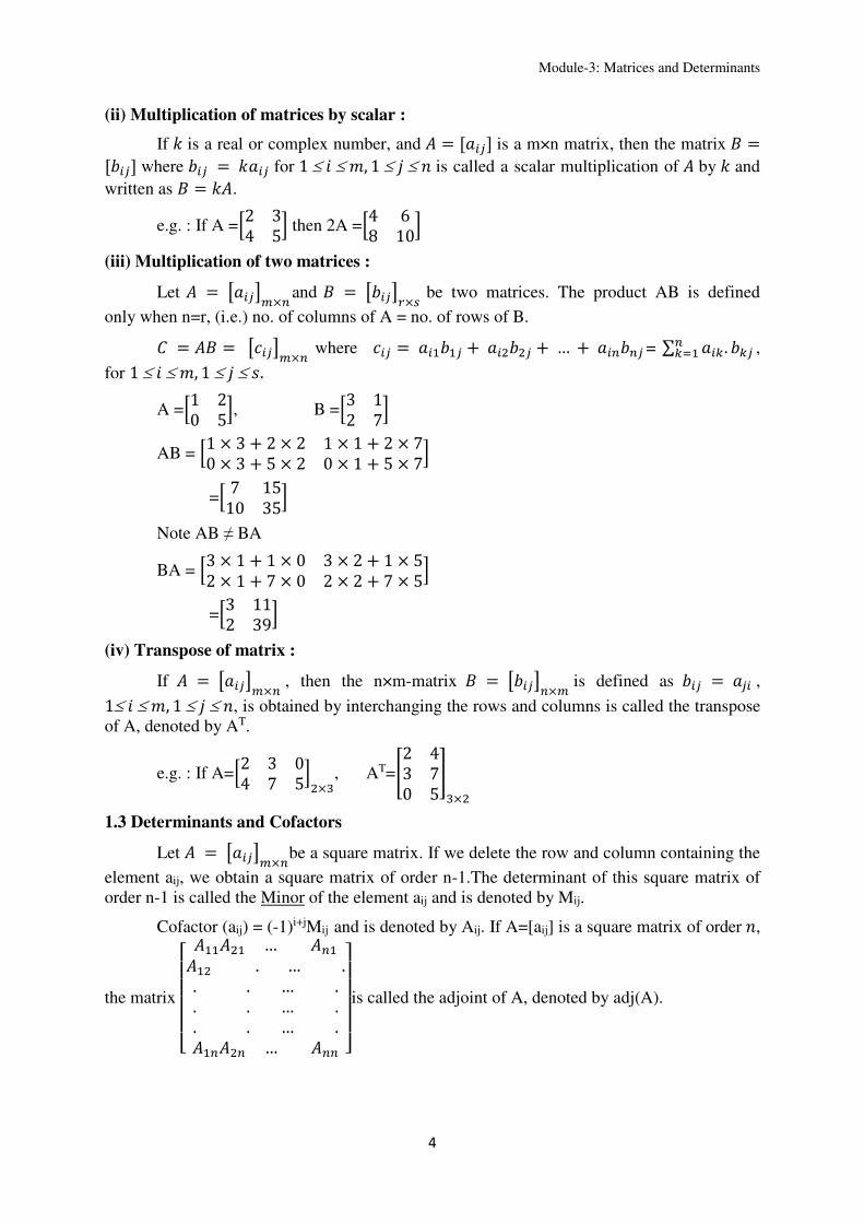
(ii) Multiplication of matrices by scalar :
If = is a real or complex number, and = [./] is a m×n matrix, then the matrix =[ ./] where ./ = =./ for 1 ≤ 9 ≤ :, 1 ≤ ; ≤ < is called a scalar multiplication of by = and
written as = =.
e.g. : If A =2 34 5 then 2A =4 68 10 (iii) Multiplication of two matrices :
Let = 2./3*×( and = 2 ./3@×A be two matrices. The product AB is defined
only when n=r, (i.e.) no. of columns of A = no. of rows of B. = = 2!./3*×( where !./ = .& &/ + . / + … + .( (/ = ∑ .C. C/(CD& ,
for 1 ≤ 9 ≤ :, 1 ≤ ; ≤ E. A =1 20 5, B =3 12 7
AB = 1 × 3 + 2 × 2 1 × 1 + 2 × 70 × 3 + 5 × 2 0 × 1 + 5 × 7 = 7 1510 35
Note AB ≠ BA
BA = 3 × 1 + 1 × 0 3 × 2 + 1 × 52 × 1 + 7 × 0 2 × 2 + 7 × 5 =3 112 39
(iv) Transpose of matrix :
If = 2./3*×( , then the n×m-matrix = 2 ./3(×* is defined as ./ = /. , 1≤ 9 ≤ :, 1 ≤ ; ≤ <, is obtained by interchanging the rows and columns is called the transpose
of A, denoted by AT.
e.g. : If A=2 3 04 7 5×F, AT=2 43 70 5F×
1.3 Determinants and Cofactors
Let = 2./3*×(be a square matrix. If we delete the row and column containing the
element aij, we obtain a square matrix of order n-1.The determinant of this square matrix of
order n-1 is called the Minor of the element aij and is denoted by Mij.
Cofactor (aij) = (-1)i+jMij and is denoted by Aij. If A=[aij] is a square matrix of order <,
the matrix
#$$$$%
&&& … (&& . … .. . … .. . … .. . … .&(( … (( +,,,,-is called the adjoint of A, denoted by adj(A).

Module-3: Matrices and Determinants
5
1.4 Inverse of a square matrix :
A square matrix A of order < is said to be invertible, if there exists a square matrix B
of order < such that = = G( and is called the inverse of and is denoted by H&.
If A is non-singular square matrix, then H& exists and H& = &|I| . "; (). 1.5 Rank of a Matrix :
Rank of a matrix A is said to be r, if A satisfies the following conditions:
i) There exists an 8 × 8 submatrix whose determinant is non-zero.
ii) The determinant of every (r+1)×(r+1)submatrix is zero.
In other words, order of the determinant of the largest submatrix of A which does not
vanish is called the rank of the matrix and is denoted by 8().
Note that 8() ≤ :9< (:, <) where A is of order m×n.
e.g. Find r(A) using determinants of minors.
A= 2 3 43 1 2−1 2 2
Since A is 3 × 3, 8()≤3
||= 2 3 43 1 2−1 2 2 = 2(2-4)-3(6+2)+4(6+1)
=2(-2)-3(8)+4(7)
= -4 – 24 + 28 = 0 ∵ || =0, r(A)≤2.
Consider the submatrix order 2×2 :
K2 43 2K = 4-12 ≠ 0.
Since determinant of 2×2 order matrix is not equal to zero, 8() = 2.
1.6 Elementary Row(Column) Operations:
Let A be an m×n order matrix. An elementary row (column) operation on A is one of
the following three types:
i) Interchange of any two rows(columns) denoted by Ri↔Ri (Ci↔Cj).
ii) Multiplication of row(column) by a non-zero element c, denoted by Ri→cRi
(Ci→cCi).
iii) Addition of any multiple of one row(column) with other row Ri→Ri + kRj
(Ci→Ci + kCj).
By applying any of these elementary operations, the rank of matrix is not affected.
Hence, “By successive application of elementary row and column operations, any non-zero
m×n matrix A can be reduced to a diagonal matrix D in which the diagonal entries are either
0 or 1 and all the 1’s precede all the zeros on the diagonal.

Module-3: Matrices and Determinants
6
In other words, the non-zero m×n matrix is equivalent to a matrix of the form G@ 00 0 where Ir is the 8 × 8 - identity matrix and 0 is the zero matrix. This is called the
canonical form of the matrix.
Two matrices A and B of the same order are said to be equivalent if B can be obtained
from A by a finite number of elementary transformation.
Definition (Rank of a matrix) :
If A is a m×n matrix, then the unique non-negative integer r such that A ~ G@ 00 0 is said to
be the rank of A. The matrix is called as the canonical form of A.
Example: Find the rank of A = 1 1 1 14 1 0 20 3 4 2. A = 1 1 1 14 1 0 20 3 4 2
A is 3×4 matrix.∴ Clearly 8() ≤3. A ~ 1 1 1 10 − 3 − 4 − 20 3 4 2 R2→R2 - 4 R1
~ 1 1 1 10 − 3 − 4 − 20 0 0 0 R3→ R3+ R2
~ 1 1 1 10 1 4/3 2/30 0 0 0 R2→R2 /(-3)
~ 1 0 0 00 1 4/3 2/30 0 0 0 C2→ C2 – C1 , C3→ C3 – C1, C4→ C4 – C1
~ 1 0 0 00 1 0 00 0 0 0 C3→ C3 – 4/3 C2, C4→ C4 – 2/3 C2
A ~ G@ 00 0 ∴ r(A) = 2.
1.7 Solving systems of equations
Given a system of equations of the form N = , where A is an m×n coefficient
matrix, X -unknown vector of (n×1) order and B-a vector of (m×1) order.
A=
#$$$$%
&&& … &(& … (. . … .. . … .. . … .*&* … *(+,,,,-, X=
#$$$$%O&O...O(+,,
,,-, B=
#$$$$%
& ... *+,,,,-

Module-3: Matrices and Determinants
7
The m×(n+1) matrix, denoted [A|B] is called the augmented matrix of the system
[A|B]=
#$$$$%
&&& … &( && … ( . . … . .. . … . .. . … . .*&* … *( * +,,,,-
If the system has atleast one solution, then the system is called consistent, otherwise
the system is said to be inconsistent.
A system AX=B
(i) is consistent iff 8() = 8<= ([|]).
(ii) has a unique solution iff 8() = 8([|]) = <, the number of unknowns (In
this case m ≥ n).
(iii) has infinitely many solutions if and only if 8() = 8([|]) < :9<:, <.
Remark1: If : = < and the 8() = <, then the 8() = 8([|]) = < and hence the system N = has a unique solution and the solution is given by N = H&.
Remark 2: To test whether the system N = , when : = <, is consistent or not, and if it is
consistent, then to find the solutions of the system, we can use elementary row operation to
the augmented matrix [|] and reduce in [|] to a triangular matrix.
Note:
i) If || ≠0, then the system has a unique solution, ∴ It is consistent.
ii) If || = 0 and if 8() = 8([|]), then the system has infinitely many solutions
and hence consistent.
iii) If || = 0 and if 8() ≠ 8([|]) then the system has no solution and hence the
system is inconsistent
References:
1. J.P. Singh, Discrete Mathematics for Under graduates, Ane Books, 2014.
2. P.B. Bhattacharya, S,.K.Jain, S.R. Nagpaul, First Course in Linear Algebra,
Wiley, 1983.
3. G. Hadley, Linear Algebra, Narosa Publishing, 1992.

Module-3: Matrices and Determinants
8
Assignment on Matrices and Determinants
1) If A = 3 1−1 2, show that A satisfies A2-5A+7I = 0. Hence determine A3 and A-1.
2) Find the inverse of 1 2 −13 8 24 9 −1, if it exists, using adjoint.
3) Find the rank of matrix using elementary row/column operation:
S 1 2 − 2 32 5 − 4 6−1 − 3 2 − 22 4 − 1 6 T
4) Find rank of the matrix 1 1 1 14 1 0 2 0 3 4 2 by examining the determinant of minors.
5) For what value of λ and µ, the system of equations: O + U + V = 6 O + 2U + 3V = 10 O + 2U + λ z = X
(i) Consistent
(ii) Consistent with unique solution
(iii) Inconsistent
6) Apply the properties of determinants and calculate :
i) A= 1 2 34 5 67 8 9, ii) B= 1 0 10 1 00 0 1, and iii) C = 2 3 42 + 3 + 42 ! + 3 " + 4.

Module-4: Complex Numbers
1
Module-4
Pretest on Complex Numbers
1. What are the roots of Find the value of + 1 = 0 ?
2. Find real numbers and such that 3 + 2 − + 5 = 7 + 5. 3. Perform each of the indicate operations
(a) 3 + 2 + −7 − (b) −7 − − 3 + 2
4. Find the value of (i) 1 + (ii) −2 + 34 −
5. What is the cube roots of unity ?
6. Find and of following complex number
(a) = (b) = 7. Find all solutions of the equation = −1 + .
8. Find the real and imaginary parts and of given complex functions of and
(a) ! = 6 − 5 + 9 (c) ! = −3 − 2 − (b) ! = − 2 + 6 (d) ! = −

Module-4: Complex Numbers
2
Module-4
Complex Numbers
Lectures required -03
Note: We use ∶= to abbreviate “defined by” or “written as”.
Definition of complex numbers:
Consider ordered pairs of real numbers (, . The word ‘ordered’ means that
(, , , are distinct unless = . We denote the set of all ordered pairs of real numbers
byℂ. We shall call ℂ as the set of all complex numbers. In ℂ, we define addition + and
multiplication (× or juxtaposition) between two such ordered pairs , , , by
+ = + , + (1)
and
, , = − , + . (2)
If = , and = , , then we say that
= ⇔ = and = .
In particular, = = 0, 0 ⇔ = 0 and = 0. We can easily check the following simple properties for equality of ordered pairs making it an
equivalence relation: For , /01 in ℂ, I. =
II. = ⇒ = III. = and = ⇒ = .
The associative and commutative laws for addition and the multiplication and distributive laws
etc., follow easily from the properties of field of real numbers ℝ. Further, it is clear from
equations (1) and (2) that (0,0) is the additive identity, (1,0) is the multiplicative identity, −, − is the additive inverse of = , and
4 ∶= 55676 , − 75676
is the multiplicative inverse of = , ≠ 0,0. • There is a unique complex Number, say , such that + = . If 9 = 9, 9
(: = 1, 2, 3), then = − , − and is denoted by − . ;<=>?/@>A0B

Module-4: Complex Numbers
3
• for ≠ 0, 0, there is a unique such that = . In fact , = . 1/ Since = . . 1/ = D . 1/ E. = 1. = . The complex number is
otherwise written as = / . The symbol commonly used for a complex number is not , but + , , real.
Following Euler, we define ∶= 0, 1 in the complex number system ℂ of ordered pairs. We
write the real number as , 0. Then accoridng to (2)
= (0, 1) (0 1)= −1, 0, = . = −1, 00, 1 = 0, −1, and O = . = 1, 0. Also, + = , 0 + 0,1, 0 = , .The above discussion
shows that ℂ is also a field.Further,writing a real number as , 0 and noting that
, 0 + , 0 = + , 0 and , 0 , 0 = , 0,
ℝ Turns out to be a subfield of ℂ. The association ↦ , 0 shows that we can always treat ℝ
as a subset of ℂ. Complex numbers of the form , 0 are said to be purely real or just real.
Those of the form 0, are said to be purely imaginary whenever ≠ 0. In particular, we have
with the above identification of ℝ, = −1. Every (complex number) = , ∈ ℂ, denoted
now by + , admits a unique representation.
, = , 0 + 0, 1, 0 = + , with , R ℝ.
‘Zero’ viz. 0, 0 = 0 + 0 is the only complex number both real and purely imaginary. The
conjugate of a complex number = + is the complex number ∶= − . Note that =
if and only if + = − , i.e = 0 i. e. is purely real. The inverse or reciprocal of a
complex number = + ≠ 0 is
1 = = − + = + − S + T, which was defined earlier as the multiplicative inverse of . we call and the real part and
imaginary part of = + , respectively. We write
Re ∶= and Im ∶= ; Re = 44 and Im z = 44 .
We know that ordered pairs of real numbers represent points in the geometric place referred to a
pair of rectangular axes. We then call all the collection of ordered pairs as ℝ and the two axes
as the -axis and − /W. Because , 0 ∈ ℝ corresponds to real numbers, the - axis called
the real axis and since = 0, ∈ ℝ is purely imaginary, the y-axis is called the imaginary
axis.
Now, we can visualize ℂ as a plane with + as points in ℝ and we simply refer to it as the
finite complex plane or simply complex plane. Depending on the problems on hand, we use + or , ), to represent a complex number.

Module-4: Complex Numbers
4
Theorem 1: The field ℂ cannot be totally ordered in consistence with the usual order on ℝ.
(Total ordering means that if / ≠ = then either / < = or / > =.
Proof: Suppose that such a total ordering exists on ℂ . Then for ∈ ℂ we would have either > 0 A? < 0 since ≠ 0.This means that in either case
−1 = ∙ = −− > 0
which is not true in ℝ. This observation shows that such an ordering in impossible in ℂ .
Theorem 1 means that the expressions > or < have to meaning unless and are
real.
Concepts of modulus / absolute value:
The modulus or absolute value of ∈ ℝ is defined by
|| = \ if ≥ 0− if < 0. As it stands, there is no natural generalized of |∙| to ℂ, because, as we have seen in Theorem 1,
there is no total ordering on ℂ. However we interpret || geometrically as the distance from to
the origin (zero) of the real line. It is this fact which leads us to define the modulus of a complex
number = + ∈ ℂ by || = √ = ` + .
Circles Suppose a = a + a, Since
| − a| = ` − a + − a is the distance between the points = + and
a = a + a, the points = + that satisfy the equation
| − a| = b, b > 0. (3)
Lie on a circle of a radian b centered at the point a see Figure (1)
Fig 1
| − a| = b
a b
Module-4: Complex Numbers
5
Circle of raids b
Example 1: Two circles
/ || = 1 is an equation of a unit circle centered at the origin.
= by rewriting | − 1 + 3| = 5 as | − 1 − 3| = 5, we see from (3)
That the equation describes a circle of radius 5 centered at the point a = 1 − 3.
Disks and Neighborhoods:
The points that satisfy the in equality | − a| ≤ b can be either on the circle | − a| = b or within the circle. We say that the set of points defined by | − a| ≤ b is a disk
of radius b centered at a. But the points that satisfy the strict inequality | − a| < b lie
within, and not on a circle of radius b centered at the point a. This set is called a neighborhood
of a. Occasionally, we will need to use a neighborhood of a that also excludes a such a
neighborhood is defined by the simultaneous inequality 0 < | − a| < b and is called a deleted
neighborhood of a. For example, || < 1 defines a neighborhood of the origin, where as 0 < || < 1 defines a deleted neighborhood of the origin; | − 3 + 4| < 0.01 defines a
neighborhood of 3 − 4, whereas the inequality 0 < | − 3 + 4| < 0.01 define a deleted
neighborhood of 3 − 4. Open Sets: A point a is said to be a interior point of a set S of the complex plane if there exists
some neighborhood of a that lies entirely within S. if every point of of a set S in an interior
point, then S is said to be an open set see Figure 2 For example Re > 1 defines a right half
plane, which is an open set. If we choose, for example a = 1.1 + 2, then a neighborhood of a lying entirely in the set is defined by | − 1.1 + 2| < 0.05 See Fig. 3.On the other hand,
the set S of points in complex plan defined by Re ≥ 1 not an open set because every
neighborhood of a point lying on the line = 1 must contain a points in S and points not in S.
See Fig 1.18

Module-4: Complex Numbers
6
Figure 2 Open set
| − 1.1 + 2| < 0.05
Figure 3 Open set with magnified view of point near = 1
Figure 4 Set S not Open

Module-4: Complex Numbers
7
If every neighborhood of a point a of a set S contains at least one point of S, and at least one
point not in S then, a is said to be boundary point of S. A point that is neither an interior
point nor a boundary point of a set S is said to be an exterior point of S; in other words, a is an
exterior point of a set S if there exists some neighborhood of that Contains no points of S. Figure
5 shows a typical set S with Interior, boundary, and exterior.
Figure 5 Interior, boundary, and exterior of set S
Annulas: The set < of points satisfying the inequality b < | − a| lie exterior to the circle of
radius b centered at a, whereas the set < of points satisfying | − a| < b lie interior to the
circle of radius b centered at a. Thus, if 0 < b < b, the list of points satisfying the
simultaneous inequality
b < | − a| < b (4)
is the intersection of the sets <and <. This intersection is an open circular ring centered at a.
Figure 6 illustrates such a ring centered at the origin. The set defined by (4) is called an open
circular annulus. By allowing b = 0, we obtain a deleted neighborhood of a.
Module-4: Complex Numbers
8
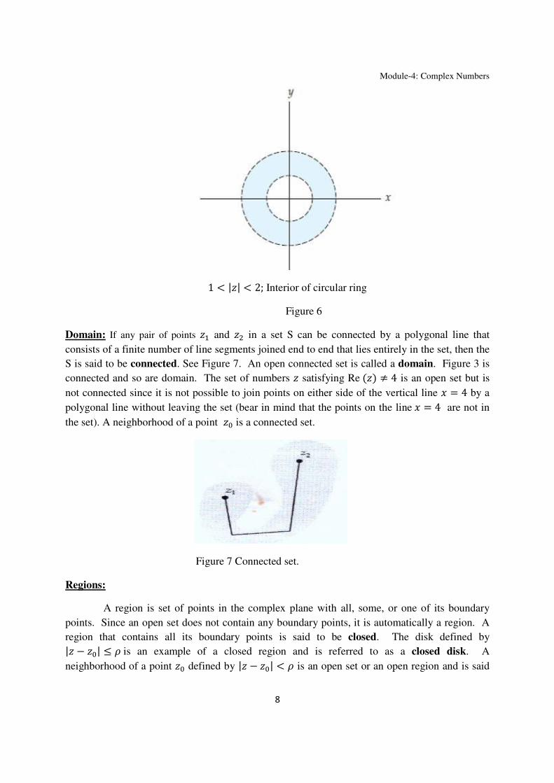
1 < || < 2; Interior of circular ring
Figure 6
Domain: If any pair of points and in a set S can be connected by a polygonal line that
consists of a finite number of line segments joined end to end that lies entirely in the set, then the
S is said to be connected. See Figure 7. An open connected set is called a domain. Figure 3 is
connected and so are domain. The set of numbers satisfying Re ≠ 4 is an open set but is
not connected since it is not possible to join points on either side of the vertical line = 4 by a
polygonal line without leaving the set (bear in mind that the points on the line = 4 are not in
the set). A neighborhood of a point a is a connected set.
Figure 7 Connected set.
Regions:
A region is set of points in the complex plane with all, some, or one of its boundary
points. Since an open set does not contain any boundary points, it is automatically a region. A
region that contains all its boundary points is said to be closed. The disk defined by | − a| ≤ b is an example of a closed region and is referred to as a closed disk. A
neighborhood of a point a defined by | − a| < b is an open set or an open region and is said
Module-4: Complex Numbers
9
to be an open disk. If the center a is deleted from either a closed disk or an open disk, the
regions defined by 0 < | − a| ≤ b or | − a| < b are called punctured disks. A punctured
open disk is the same as a deleted neighborhood of a. a region can be neither open nor closed;
the annular region defined by the inequality 1 ≤ | − 5| < 3 contains only some of its boundary
points (the points lying on the circle| − 5| = 1), and so it is neither open nor closed. In (4) we
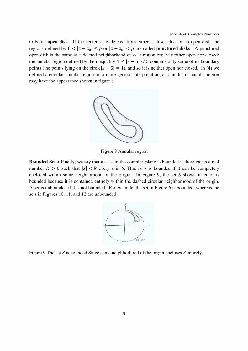
defined a circular annular region; in a more general interpretation, an annulus or annular region
may have the appearance shown in figure 8.
Figure 8 Annular region
Bounded Sets: Finally, we say that a set s in the complex plane is bounded if there exists a real
number > 0 such that || < every z in S. That is, s is bounded if it can be completely
enclosed within some neighborhood of the origin. In Figure 9, the set S shown in color is
bounded because it is contained entirely within the dashed circular neighborhood of the origin.
A set is unbounded if it is not bounded. For example, the set in Figure 6 is bounded, whereas the
sets in Figures 10, 11, and 12 are unbounded.
Figure 9 The set S is bounded Since some neighborhood of the origin encloses S entirely.

Module-4: Complex Numbers
10
Figure 10 Im < 0 ; lower half plan
Figure 11. −1 < < 1 ; infinite vertical strip
Figure 12. || > 1 ; exterior of unit circle

Module-4: Complex Numbers
11
Complex Function: One of the most important concepts in matchematics is that of a function.
You may recall from previous courses that a function is a certain kind of corresspondence
between two sets; more specifically:
A function ! from a set A to a set B is a rule of correspondence that assign to each element in a
one and only one element in B.
We often think of a function as a rule or a machine that accepts inputs from the set A and returns
outputs in the set B. In elementary calculus we studied functions whoe inputs and outputs were
real numbers. such functions are called real-valued functions of a real variable. In this section
we begin our study of functions whose inputs and outputs are complex numbers. Naturally, we
call these functions complex functions of a complex variable, or complex functions for short.
As we will see, many interesting and useful complex functions are simply generalizations of
well-known functions from calculus.
Function: Suppose that ! is a function from the set A to the set B . If ! assigns to the element a
in A the element = in B, then we say that = = !/. The set A-the set of inputs is called the
domain of ! and the set of images in B the set outputs is called the range of !. We denote the
domain and range of a function ! by Dom ! and Range !, respectively. As an example,
consider the “squaring” function ! = defined for the real variable x. Since any real
number can be squared, the domain of f is the set R of all real numbers. That is , Dom (f) = A =
R. The range of f consists of all real numbers where is a real number. Of course, ≥ 0 for
all real , and it is easy to see from the graph of ! that the range of f that the range of f is the
set of all nonnegative real numbers. Thus, Range ! is the interval (0, ∞. The range of ! need
not be the same as the set B. For instance, because the interval (0, ∞ is a subset of both R and
the set C of all complex numbers, f can be viewed as a function from A=R to B=R or ! can be
viewed as a function from A=R to B=C. In both cases, the range of ! is contained in but not
equal to the set B.
As the following definition indicates, a complex function is a function whose inputs and
outputs are complex numbers.
Definiton 1 Complex function: A complex function is a function ! whose domain and range
are subsets of the set C of complex numbers.
A complex function is also called a complex-valued function of a complex variable. for
the most part we will use the usual symbols !, f, and ℎ to denote complex functions. In
addition, inputs to a complex function f will typically be denoted by the variable and outputs by
the variable = !. When referring to a complex function we will use three notations
interchangedably, for example, ! = − , = − , or, simply, the function − . Throughout this text the notation = ! will be reserved to represent a real-valued function of
a real variable .
Module-4: Complex Numbers
12
Example1. Complex function: (a) The expression − 2 + can be evaluated at any
complex number z and always yields a single complex number, and so ! = − 2 +
define a complex function. Values of f are found by using the arithmetic operations for complex
numbers . For instance, at the points = and = 1 + we have:
! = − 2 + = −1 − 2 + 1 = −2 and !1 + = 1 + − 2 + 1 + = 2 − 1 − 3 = −1 − (b) The expression f = + 2 defines a complex function .Some values of f are:
f = + 2 = + 20 =
and f2 − 3 = 2 − 3 + 2 2 − 3 = 2 − 3 + 22 = 6 − 3. Real and Imaginary Parts of a Complex Function: It is often helpful to express the inputs and
the outputs a complex function in terms of their real and imaginary parts. If = ! is a
complex function, then the image of a complex number = + under f is a complex
number = + . By simplifying the expression ! + , we can write the real variables and in terms of the real variables x and . For example, by replacing the symobl with + , we can express any complex function = , we obtain:
= + = + = − + 2. (5)
From (5) the real variables and are given by = − and = 2 respectively. This
example illustrates that, if = + = + is a complex function, then both and are
real functions of the two real variables and y. That is, by setting = + , we can express
any complex function = ! in terms of two real funtions as:
! = , + , . (6)
The functions , and , in (6) are called the real and imaginary parts of f ,
respectively.
Example 2. Real and imaginary parts of a function:
Find the real and imaginary parts of the functions: (a) ! = − 2 + and
(b) f = + 2 . Solution. In each case, we replace the symbol by + , then simplify.
(a) ! = + − 2 + + = − 2 + − + 2 − − 2. So ,, = − 2 + − and , = 2 − − 2.
(b) Since f = + + 2 + = 3 + , we have , = 3 and , = .
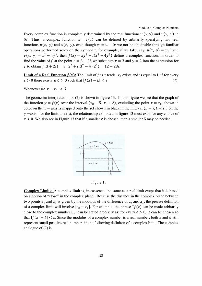
Module-4: Complex Numbers
13
Every complex function is completely determined by the real functions , and , in
(6). Thus, a complex function = ! can be defined by arbitarily specifying two real
functions , and , , even though = + we not be obtainable through familiar
operations performed soley on the symbol z. for example, if we take, say, , = and , = − 4, then ! = + − 4 define a complex function. in order to
find the value of f at the point = 3 + 2, we substitute = 3 and = 2 into the expression for ! to obtain !3 + 2 = 3 ∙ 2 + 3 − 4 ∙ 2 = 12 − 23. Limit of a Real Function hi: The limit of f as x tends a exists and is equal to L if for every j > 0 there exists / k > 0 such that |! − l| < j (7)
Whenever 0<| − a| < k. The geometirc interpretation of (7) is shown in figure 13. In this figure we see that the graph of
the function = ! over the interval a − δ, a + δ, excluding the point = a, shown in
color on the − axis is mapped onto the set shown in black in the interval l − j, l + j, on the −axis. for the limit to exist, the relationship exhibited in figure 13 must exist for any choice of j > 0. We also see in Figure 13 that if a smaller j is chosen, then a smaller δ may be needed.
Figure 13.
Complex Limits: A complex limit is, in eassence, the same as a real limit exept that it is based
on a notion of “close” in the complex plane. Because the distance in the complex plane between
two points and is given by the modulus of the difference of and , the precise definiton
of a complex limit will involve | − |. For example, the phrase “! can be made arbitarily
close to the complex number L,” can be stated precisely as: for every j > 0, can be chosen so
that |! − l| < j. Since the modulus of a complex number is a real number, both j and k still
represent small positive real numbers in the following definiton of a complex limit. The complex
analogue of (7) is:
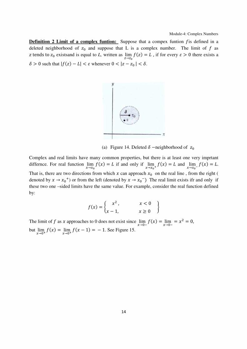
Module-4: Complex Numbers
14
Definition 2 Limit of a complex funtion: Suppose that a compex funtion !is defined in a
deleted neighborhood of a and suppose that L is a complex number. The limit of ! as tends to a existsand is equal to L, written as lim4→4s ! = l , if for every j > 0 there exists a
k > 0 such that |! − l| < j whenever 0 < | − a | < k.
(a) Figure 14. Deleted k −neighborhood of a Complex and real limits have many common properties, but there is at least one very imprtant
differnce. For real function lim5→5s ! = l if and only if lim5→5st ! = l and lim5→5su ! = l. That is, there are two directions from which can approach a on the real line , from the right (
denoted by → a) or from the left (denoted by → a The real limit exists ifr and only if
these two one –sided limits have the same value. For example, consider the real function defined
by:
! = v , < 0 − 1, ≥ 0 w
The limit of ! as approaches to 0 does not exist since lim5→a ! = lim5→a = = 0, but lim5→at ! = lim5→at ! − 1 = − 1. See Figure 15.

Module-4: Complex Numbers
15
Figure 15. The limit of f does not exist as x approaches 0.
For limits for complex functions, z is allowed to approach a from any direction in the complex
plane, that is, along any curve or path through a. See Figure 16.In orer that lim4→4s ! exists and
equals l along every possible curve through a. Put in a negative way:
Figure 16. Different ways to approach a in a limit.
Example 3. A Limit That does Not Exist
Show that lim4→a 44 does not exist.
Solution: We show that this limit does not exist by finding two different ways of letting
approach 0 that yield different values of lim4→a 44 .First, we let approach 0 along the real axis.
That is we consider complex numbers of the form = + 0 where the real number is
approaching 0. for these points we have:
lim4→a 44 = lim5→a 5a5a = lim5→a1 = 1. (8)
Module-4: Complex Numbers
16
On the other hand, if we let = 0 + where the real number is approaching 0. For this
approach we have:
lim4→a 44 = lim5→a a7a7 = lim7→a−1 = −1. (9)
Since the values in (8) and (9) are not the same, we conclude that lim4→a 44 does not exist.
Example 4 An Epsion-Delta Prof of a Limit:
Prove that lim4→2 + = 1 + 3. Solution According to definition 2.; lim4→2 + = 1 + 3, if, for every j > 0, there is a k >0 such that |2 + − 1 + 3| < j when ever 0 < | − 1 + | < k. proving that the limit
exists requires that we find an appropriate value of k for a given value of j . In other words, for
a given value of j we must find a positive number k with the property that if 0 < | − 1 + | <k, then |2 + − 1 + 3| < j. One way of finding k is to “work backwards.” The idea is to
start with the inequality:
|2 + − 1 + 3| < j (10)
and then use properties of complex numbers and the modulus to manipulate this inequality until
it involves the expression | − 1 + |. Thus, a natural first step is to factor 2 + out of the
left-hand side of (10):
|2 + |. | − | < j. (11)
Because |2 + | = √5 and = 1 + , 11is equivalent to: √5. | − 1 + | < j or | − 1 + | < |√. (12)
Thus, (12) indicates that we should take k = |√. Keep in mind that the choice of k is not unique.
Our choice of k = |√ is a result of the particular algebraic manipulations that we employed to
obtain (12). Having found k we now present the formal proff that lim4→2 + = 1 + 3. that
does not indicate how the choice of k was made:
Given j > 0, let k = |√ . if 0 < | − 1 + | < k, then we have | − 1 + | < |√.
Multiplying both sides of the last inequality by |1 + | = √5 we obtain:
|2 + |. | − 1 + | < √5. |√. or |2 + − 1 + 3| < j.
Module-4: Complex Numbers
17
Therefore, |2 + − 1 + 3| < j whenever 0 < | − 1 + | < k, So, according to
Definition 2., we have proven that lim4→2 + = 1 + 3. Real Multivariable Limits: The epsilon-delta proof from Example 4 illustrates the important
fact that alghouth the theory of complex limits is based on Definition 2, this definition does not
provide a convenient method for computing limits. We now present a practical method for
computing complex limits in Theorem 2. In addition to being a useful computational tool, this
theorem also establishes an important connection between the complex limit of ! =, + !, and the real limits of the real- valued function of two real variables , and , . Since every complex function is completely determined by the real
functions and .
Before stating Theorem 2. we recall some of the important concepts regarding limits of real-
valued functions of two real variables , . The following definition of lim5,7→5s ,7s , = l is analosous to both equation (7) and Definiton 2.
Limit of the real function i, : The limit of as , tends to (a, a) exists and is equal to the real number l if for every j >0 there exists a k > 0 such that
| − − l| < j whenever 0 < ` − a + − a < k. (13)
The expression ` − a + − a in (13) represents the distance between the points , and a, a in the Cartesian plane. Using (13), it is relatively easy to prove that:
lim5,7→5s ,7s 1 = 1, lim5,7→5s ,7s = a, /01 lim5,7→5s ,7s = a (14)
If lim5,7→5s ,7s, = l and lim5,7→5s ,7s, = , then (13) can also be used to show:
lim5,7→5s ,7s @ , = @l, @ a real constant, (15)
lim5,7→5s ,7s, ± , = l ± , (16)
lim5,7→5s ,7s , ∙ , = l ∙ , (17)
and lim5,7→5s ,7s 5,75,7 = , ≠ 0. (18)
Limits involving polynomial expressions in and can be easily computed using the limits in
(14) combined with properties (15)-(18). For example,
Module-4: Complex Numbers
18
lim5,7→,3 − = 3 S lim5,7→,T S lim5,7→,T S lim5,7→,T − lim5,7→,
= 3∙ 1 ∙ 2 ∙ 2 − 2 = 10. In general, if , is a two-variable polynomial function, then (14)-(18) can be used to show
that
lim5,7→5s ,7s, = a, a (19)
If , and , are two-variable polynomial functions and a, a ≠ 0, then equations
(19) and (18) give:
lim5,7→5s ,7s 5,75,7 = 5s,7s5s,7s (20)
We now present Theorem 2., which relates real limits of , and , with the complex
limit of ! = , + , . Theorem 2. Real and imaginary parts of a Limit:
Suppose that ! = , + , , a = a + a, /01 l = a + a. Then lim4→4s! = l
if and only if
lim5,7→5s ,7s, = a and lim5,7→5s ,7s , = a . Theorem 2. has many uses. First and foremost , it allows us to compute many complex limits by
simply computing a pair of real limits.
Example 5: Using Theorem 2. to compute a Limit:
Use Theorem 2. to compute lim4→ + . Solution: Since ! = + = − + 2 + 1, we can apply Theorem 2. with
, = − , , = 2 + 1, and a = 1 + . Identifying a = 1 and a = 1,we find a and a by computing the two real limits:
a = lim5,7→, − and a = lim5,7→,2 + 1. Since both of these limits involve only multivariable polynomial functions, we can use (19) to
obtain:
a = lim5,7→, − = 1 + 1 = 0

Module-4: Complex Numbers
19
a = lim5,7→,2 + 1 = 2 ∙ 1 ∙ 1 + 1 = 3
and so l = a + a = 0 + 3 = 3. Therefore, lim4→ + = 3. Continuity of Complex Functions:
The definition of continuity for a complex function is, in essence, the same as that for a real
function. That is a complex function ! is continuous at a point a if the limit of ! as
approaches a exists and is the same as the value of ! at a. This gives the following definition
for complex functions.
Definition 3. Continuity of a Complex Function:
A complex function ! is continuous at a point a if lim4→4s! = !a. Analogous to real function, if a complex ! is continuous at a point , then the following three
conditions must be met.
Criteria for Continuity at a Point:
A complex function ! is continuous at a point a if each of the following three conditions hold:
(i) lim4→4s! exists, (ii) ! is defined at a, and
(iii) lim4→4s! = !a.
If a complex function ! is not continious at a point a then we say that ! is discontinuous at a.
for example, the function ! = 46 is discountinuous at = and = −. Example 6 Checking Continuity at a Point:
Consider the function ! = − + 2. In order to determine if ! is continuous at, say, the
point a = 1 − , we must find lim4→4s! and !a, then chek to see whether these two complex
values are equal. From Theorem 2.2 and the limits in (15) and (16) we obtain:
lim4→4s! = lim4→ − + 2 = 1 − − 1 − + 2 = 1 − 3. Furtheromre, for a = 1 − we have:

Module-4: Complex Numbers
20
! = !a, we conclude that ! = − + 2 is a continuous at the point a = 1 − .
Continuity of a Real Function i ,
A function F is continuous at a point a , a if
lim5,7→5s ,7s, = a , a. (21)
Theorem 3. Real and Imaginary Parts of a Continuous Function:
Suppose that ! = , + , and a = a + a. Then the complex function ! is
continuous at the point a if and only if both real functions and are contiunous at the point
(a, a).
Proof: Assume that the complex function ! is continuous at a . Then form Definition 3 we
have:
lim4→4s! = !a = a, a + a, a. (22)
By Theorem 2., this implies that:
lim5,7→5s ,7s, = a, a and lim5,7→5s ,7s , = a, a (23)
Therefore, from (21), both and are continuous a, a. Conversely, if and are
continuous at (a, a), then
lim 5,7→5s ,7s, = a, a and lim5,7→5s ,7s , = a, a.
It then follows form Theorm 2. that lim4→4s! = a, a + a, a = !a. Therefore, ! is
continuous by Definition 3.
Example 7.Checking Continuity Using Theorem 3:
Show that the function ! = is continuous on C.

Module-4: Complex Numbers
21
Solution: According to Theorem 3, ! = = + = − is continuous at a = a +a if both , = and , = − are continuous at (a, a). Because and are two-
variable polynomial functions, it follows from (19) that:
lim5,7→5s ,7s, = a and lim5,7→5s ,7s , = −a.
This implies that and are continuous at (a , a), and, therefore, that ! is continuous at a =a + a by the Theorem 3. Since a = a + a was an arbitary point, we conclude that the
function ! = is continuous on C.
Theorem 4 Properties of Complex Limits
Suppose that ! and f are complex functions. If lim4→4s! = l and lim4→4sf = , then
(i) lim4→4s@! = @l , c a complex constant,
(ii) lim4→4sD! ± fE = l ± ,
(iii) lim4→4s!. f = l. , and
(iv) lim4→4s44 = , provided ≠ 0.
Proof of (i) Each part of Theorem 4 follows from Theorem 2 and the analogous property (15)-
(18). We will prove part (i) and leave the remaining parts as exercises.
Let ! = , + , , a = a + a, l = a + a and @ = / + = .
Since lim4→4s! = l, it follows from Theorem 2 that lim 5,7→5s ,7s, = a and
lim5,7→5s ,7s , = a. By (15) and (16) ,we have
lim 5,7→5s ,7s/, − = , = /a − = a
and lim 5,7→5s ,7s/, + = , = /a + = a. However , ReD@!E = /, − = , and ImD@!E = =, + / , .Therefore,
By Theorem 2,
lim4→4s@! = /a − = a + /a + = a = @l. The algebraic properties of complex limits from Theorem 4 can also be restated in terms of
continuity of complex functions.
Module-4: Complex Numbers
22
Theorem 5: Properties of Continuous Function:
If ! and f are continuous at the point a, then the following functions are continuous at the
point a: (i) @!, @ a complex constant,
(ii) ! + f,
(iii) ! ∙ f, and
(iv) provided fa ≠ 0.
Proof of (ii) We prove only (ii); proofs of the remaining parts are similar. Since ! and f are
continuous at a we have that lim4→4s! = !a and lim4→4sf = fa. From Theorem 4 (ii), it
follows that lim4→4sD! + faE = !a + fa. Therefore, ! + f is continuous at a by
Definition 3.
Assignment
1. Draw the pair of points = / + = and = / − = in the complex plane if
/ > 0, = > 0; / > 0, = < 0; / < 0, = > 0; and / < 0, = < 0. 2. Consider the complex number = 4 + , = −2 + , = −2 − 2, O = 3 − 5. (a) Use four different sketches to plot the four pairs of points , ; , ; , ; and O,O. (b) In general, how would you describe geometrically the effect of multiplying a complex
number = + by ? By – ?
3. Under what circumstances does | + | = || + || ?
4. Without doing any calculations, explain why the inequalities |Re | ≤ || and |Im | ≤|| hold for all complex numbers . 5. Find the modulus of the given complex number.
(a). 1 − (b). O

Module-4: Complex Numbers
23
(c). 2 − − 4 1 + O (d). + .
6. Sketch the graph of the given equation in the complex plane.
(a) | − 4 + 3| = 5 (b) | + 2 + 2| = 2
(c) | + 3| = 2 (d) |2 − 1| = 4
(e) Re = 5 (f) Im = −2
In problems 7 -18 sketch the set S of points in the complex plane satisfying the given inequality.
Determine whether the set is (a) open (b) closed (c) a domain, (d) bounded, or (e) connected.
7. Re < −1 8. |Re| > 2
9. |Im| > 3 10. Re D2 + + 1E > 0
11. 2 < Re − 1 < 4 12. −1 ≤ Im < 4
13. > 0 14. Im < Re
15. 2 < | − | < 3 16. 1 ≤ | − 1 − | < 2
17. 2 ≤ | − 3 + 4| ≤ 5 18. | − | > 1
In Problems 19-25, show that the function ! is continuous at the given point.
19. ! = − + 3 − 2 ; a = 2 − 20. ! = − 4 ; a = 3 21. ! = 4 4464 ; a = 22. ! = 4 464 ; a = 1 + 23. ! = v4 4 || ≠ 13 || = 1 ; a = 1
24. ! = 4 464 || ≠ 1√ || = 1 ; a = √

Module-4: Complex Numbers
24
25. ! = − 3 + ; a = 3 − 2
Refrences:
1. Dennis G. Zill and Patrick D. Shanahan. A First Course in Complex Analysis with
Applications, Jones and Bartlett publishers Sudbury, Massachusetts
2. S. Ponnusamy. Foundations of Complex Analysis, Norasa publishers.

Module-5: Differential Equations
Module-5
Pretest on Differential Equations
Note: Find the correct answer in the following questions given below.
1. The differential equation
+ (
) + = 0 is of
(i) Order 1 and degree 3
(ii) Order 3 and degree 1
(iii) Order 2 and degree is not defined
(iv) Order 2 and degree 3
2. The differential equation of the family of circles touching the axis at origin is
(i) =
(ii) =
(iii) =
(iv) None of these
3. Find the family of curves for which the slope of the tangent at any point (, ) on it is
(i) − =
(ii) − =
(iii) + =
(iv) + =
4. The integrating factor of the differential equation (1 − ) + = , (−1 < <
1), (i)
(ii)
(iii)
(iv)
5. General solution of the differential equation
=
!" is
(i) = (tan − 1) + !"
(ii) = (tan − 1) + tan (iii) = (tan − 1) + !"
(iv) None of these.

Module-5: Differential Equations
2
Module-5
Differential Equations
Lectures required-03
An equation involving the dependent variable, the independent variable/variables and
derivatives of dependent variable w.r.t. independent variable/variables is called a differential
equation.
Ex. (a) = 3 +
(b) &'& + &'
& = (
(c) + 3 = )*+
The equations (a) and (c) are ordinary differential equations because these equations consist
of one independent variable x. Eq. (b) is a partial differential equation because it contains one
dependent variable ( and two independent variables x and y.
In this section, we shall discuss about ordinary differential equations only. Before going
further, let us discuss the following definitions:
Order: The order of a differential equation is the order of the highest derivative occurring in
the equation.
Ex. (i) The order of + ,
- + = 0 is two.
(ii) The order of .. + + = 0 is three.
Degree: The degree of a differential equation is the highest power of the highest order
derivative occurring in the given differential equation if the differential equation is a
polynomial equation in derivatives.
Ex. (i) The degree of ,- +
+ )*+ = 0 is three.
(ii) The degree of y″′+ + = 0 is not defined because the given equation is not a
polynomial equation in its derivatives.
(iii) The degree of ,- +
+ )*+ = 0 is two.

Module-5: Differential Equations
3
1. Formation of differential equations of first order
We first study how to form a differential equation if the complete primitive (or general
solution) is known.
Let the primitive of the differential equation be
/(, , ) = 0 (1.1)
Where is an arbitrary constant.
Differentiating Eq. (1.1), we obtain a relation between , , and of the form
0 ,, , , - = 0 (1.2)
Eliminating between the Eqs. (1.1) and (1.2), we obtain the following equation:
1 ,, , - = 0 (1.3)
Eq. (1.3) is a differential equation of the first order.
Example: Find the differential equation of all circles which pass through the origin and
whose centres are on the x axis.
We know that the equation of any circle passing through the origin and whose centre is on the
x axis is given by
+ + 22 = 0, (1.4)
Where 2 is an arbitrary constant.
Differentiating Eq. (1.4) w.r.t. x, we get
2 + 2 + 22 = 0. (1.5)
From Eq. (1.4), we have
22 = −( + )/ (1.6)
Substituting the expression of 22 from Eq. (1.6) in Eq. (1.5), we get
2 + − = 0,
Which is a differential equation whose primitive is given in Eq.(1.4).
Exercise:
(1) Find the differential equation corresponding to the family of curves = ( − ),
where is an arbitrary constant.
(2) Find the differential equation of all circles which pass through the origin and whose
centres are on the y axis.
(3) Find the differential equation corresponding to the family of curves = 4( + ),
where is an arbitrary constant.
Module-5: Differential Equations
4
2. Differential Equations reducible to linear form
The students have already studied about the differential equation of first order and first
degree and their solutions by the method of separation of variables, method of solving
homogeneous and linear equations. Therefore, let us discuss first the differential equations
reducible to the linear form:
The equation of the form
+ 6 = 78 (2.1)
is known as Bernoulli’s equation, where 6 and Q are functions of x alone.
Equation (2.1) can be reduced to the linear form by dividing the equation by 8 and
putting 8 equal toν. That is if are divide (2.1) by 8, we get
8 + 68 = 7 (2.2)
If we take 8 = ν, (2.2) becomes
(8)ν + 6ν = 7, + ≠ 1,
Which is a linear differential equation in ν and x.
Example: Solve + = .
Dividing by , we have
+ =
Now, taking =ν, we have
−2 = ν
This gives
− ν
+ ν = ⇒ ν −
ν = −2
Which is a linear differential equation.
The solution of this linear equation is
ν. :; = < −2. :; = + >,

Module-5: Differential Equations
5
Where :; (Integrating factor) = <!? =
and > is an arbitrary constant.
Hence, the solution of linear differential equation is
ν
= + >
And the final solution of given differential equation becomes
(2 + ) = 1.
An equation of the form /() + 6/() = 7, where P and Q are function of x only can
also be reduced to linear form.
If we take /() = @, so /() = ν
and the differential equation becomes:
ν + 6ν = 7
Which is linear in ν and x. This equation can be easily solved.
Ex. Reduce + )*+ 2 = A) in linear form.
Dividing above differential equation by A), we get
) + 2 tan =
If tan = @, then ) = ν
. Hence, the above equation becomes
ν + 2ν =
Which is linear in ν and x.
Exercise
(i) +
)*+ 2 = A)
(ii) + )*+ = A)2
(iii) = ( − )
(iv) + 3 =
3. Exact Differential Equation

Module-5: Differential Equations
6
A differential equation is said to be exact if it can be derived from its general solution directly
by differentiating without any subsequent multiplication, elimination, etc.
Thus, the differential equation
Mdx + Ndy = 0 (3.1)
is exact if there exists a function f(x,y) such that
d [f(x,y)] = Mdx + Ndy,
where M & N are functions of x and y.
Theorem: A necessary and sufficient condition for the differential equation Mdx + Ndy = 0
to be exact is
∂B∂ = ∂C
∂ . (3.2)
If the equation (1) is exact, then its general solution is
< D= + <(EFG *) H +AE A+E*+*+2 )= = ,
[Treating y as constant]
where is an arbitrary constant.
Example: (x2 – 4 xy – 2y2) dx + (y2 – 4 xy – 2x2)
∂B∂ = −4 − 4 &
∂C∂ = −4 − 4
Hence, the given equation is exact and its solution is
<( − 4 − 2)= + < = = (3.3)
In first integral of (3), we take y as a constant and after integration, we have
. − 4
− 2 + . = >
⇒ + − 6( + ) = >, >′ is arbitrary constant.
4. Integrating factor
Sometimes the equation Mdx + Ndy = 0 is not exact. But, it can be made exact by
multiplying it with a function of x and y. Such a function is known as integrating factor (IF).
In general, the differential Mdx + Ndy = 0 has an infinite number of integrating factor. But,

Module-5: Differential Equations
7
there is not a unique method to find them. Therefore, we discuss some rules to find
integrating factor for Eq. (3.1).
(i) By inspection: Sometimes an integrating factor can be found by rearranging the terms of
the given equation and/or by dividing by a suitable function of x & y.
Ex: Solve y (2xy+ ex)dx = exdy
⇒ (2xy2 + yex)dx - exdy=0
⇒ 2xdx + K?K?
= 0
= = , + K? - = 0 (Exact)
= x2 + ex/y = c.
(ii) If the equation Mdx + Ndy = 0 can be written in the form
f1(xy)ydx + f2(xy)xdy = 0,
and D − H ≠ 0, then
BC is an integrating factor.
Ex.: Find I.F. of y(1+xy)dx +x(1-xy)dy = 0.
Clearly M = (1+xy)y & N = (1-xy)y.
In this case D − H = 2 ≠ 0
Hence I.F. =
BC = .
(iii) If M and N are homogeneous in the equation Mdx + Ndy = 0 and D + H ≠ 0, then
BC is an integrating factor of the equation.
Ex.: Find integrating factor of
(x2y - 2xy2)dx - (x3 - 3x2y)dy = 0
Clearly M = x2y - 2xy2 & N = - (x3 - 3x2y) and M & N are homogeneous functions.
Now, D + H = ≠ 0.
Hence, I.F. = .

Module-5: Differential Equations
8
(iv) If C ,∂B
∂ − ∂C∂- is a function of x alone, say f(x), then < L() is an integrating factor of
the equation Mdx + Ndy = 0.
Ex. : Find integrating factor of (x2+y2 + x)dx + xydy = 0.
Clearly, M = x2+y2 + x & N = xy
Here, C ,∂B
∂ − ∂C∂- =
(2 − ) = = /().
Hence, I.F. = <"? = MNO = .
(v) If C ,∂H
∂ − ∂D∂ - is a function of y alone, say f(y), then < L() is an integrating factor of
the equation Mdx + Ndy = 0.
(vi) Let xhyk be the I.F. of the equation
xayb(mydx + nxdy) + xrys(pydx + qxdy) = 0,
where a, b , m, n, r, s, p, q are constants and h, k are unknowns.
Multiplying the diff. equation by the I.F., we get
(mxa+hyb+k+1 + pxr+hys+k+1)dx + (nxa++1hyb+k + qxr+h+1ys+k)dy = 0
Since this equation must be an exact. Therefore, the condition
∂B∂ = ∂C
∂ ,
provides
m(b+k+1)xa+hyb+k + p(s+k+1)xr+hys+k = n(a+h+1)xa+hyb+k + (r+h+1)xr+hys+k.
This will be true only when
P(QR)S8 (TU)V(WR)SX (YU) Z (4.1)
Eqs. in (4.1) determine the values of h and k.
Ex. : Find the integrating factor of
(2ydx + 3ydy) + 2xy (3ydx + 4xdy) = 0.
Let xhyk be I.F. of the equation. Therefore, the equation
(2xhyk+1 + 6xh+1yk+2)dx + (3xh+1yk + 8xh+2yk+2) dy = 0

Module-5: Differential Equations
9
must be exact.
Clearly, M = 2xhyk+1 + 6xh+1yk+2 & N = 3xh+1yk + 8xh+2yk+2.
By the condition ∂B∂ = ∂C
∂ , we get
2(k+1) xhyk +6(k+2) xh+1yk+1 =3(h+1) xhyk +8(h+2) xh+1yk+1,
which gives 3h-2k= -1 and 4h-3k= -2.
After solving these equations, we get
h=1 & k=2.
Hence, I.F. = xhyk = xy2
5. Differential equations of the first order but not of the first degree.
The general first order differential equation of the degree > 1 is
[ ,-8 + ,
-8 + ,-8 + ⋯ + 8 ,
- + 8 = 0 (5.1)
where a0, a1, a2,... an are functions of x and y.
In this section, we shall discuss the following solutions of Eq. (5.1).
(i) Equation solvable for ]^]_
Let = `
then Eq. (5.1) becomes
a0 pn+ a1p
n-1+..... an-1p+ an =0. (5.2)
Suppose (5.2) is solvable for p then it can be written as :
(p-f1(x,y)) (p-f2(x,y))...... (p-fn(x,y))=0 (5.3)
Equating each factor of Eq. (5.3) to zero, we get n equations of the first order and first degree.
Suppose the solutions of resulting n equations are respectively,
F1(x,y,c1)=0, F2(x,y,c2)=0 ...... Fn(x,y,cn)=0. (5.4)
In Eq. (5.4), c1, c2, ..... ,cn are arbitrary constants of integration.

Module-5: Differential Equations
10
Without loss of generality, we can replace the arbitrary constants, c1, c2, c3, .... cn by single
arbitrary constant C. Therefore, the n solutions given in Eq. (5.4) can be put in the form
F1(x,y,c)=0, F2(x,y,c)=0 ...... Fn(x,y,c)=0 (5.5)
The solution of Eq. (5.2) can evidently be put in the form
F1(x,y,c) F2(x,y,c) F3(x,y,c)..... Fn(x,y,c)=0 (5.6)
Ex. 1 4 ,- = (3 − )
⇒ 4 ` = (3 − )
⇒ p = ± T√
⇒ dy = ± c √ − T!"/
Z =
⇒ y+c = ±d/ − /e
⇒ (y+c) = ±√( − )
⇒ (y+c)2 = x (x-a)2 (general solution)
(ii) Equation solvable for y
Suppose the given differential equation f(x,y,p) =0 is solvable for y. Thus it can be put in the
form
y = F (x,p), (5.7)
where p = .
Differentiating Eq. (5.7) w.r.t. x, we get an equation in the form:
p = ∅ ,, `, V-. (5.8)
In Eq. (5.8) only two variables p and x are present . It may be possible to find the solution of
Eqn. (5.8) in the form:
ψ (x, p, c) = 0, (5.9)
where c is arbitrary constant.
The elimination of p between Eqs. (5.7) and (5.9) gives us the required solution.

Module-5: Differential Equations
11
If elimination is not possible, the Eqs. (5.7) and (5.9) may be taken as solution which give x
and y in terms of parameter p.
Ex. 1. Solve y+px = x4p2.
⇒ y = x4p2-px (5.10)
Diff. w.r.t. x and taking p for dy/dx, we get
P = 4x3p2+2x4pV – p-x
V
2P(1-2x3p)+x,V- (1-2x3p) = 0
⇒ (1-2x3p) g2` + Vh = 0 (5.11)
The second factor of Eq. (5.11) contains V, so from this equation, we have
2` + V = 0
⇒ V =` + 2
= 0 ⇒ p = c/x2 (5.12)
Eq. (5.10) and Eq. (5.12) gives
xy ± c = c2x
which is the solution of the problem.
(iii) Equations solvable for x.
If the given equation is solvable for y, then we can put that equation in the form
x = f(y,p) (5.13)
Differentiating (1) w.r.t. y and writing 1/p for , we get
V = ∅ ,, `, V
- (5.14)
Suppose that the solution of Eq. (5.14) is possible and let the solution be
ψ (y, p, c) = 0 (5.15)
where c is arbitrary constant.

Module-5: Differential Equations
12
The elimination of p between Eqs (5.13) and (5.14) gives us the required solution. If the
elimination of p is not possible, then we solve (5.13) and (5.15) to express x and y in terms of
parameter p.
Ex. Solve y = 2px + p2y
⇒ 2x = -py + y/p (5.16)
Diff. w.r.t. y, we get
V = −` − i
+ V −
Vi ,
⇒ (1 + 1/`) g` + ,i-h = 0. (5.17)
Neglecting first factor of Eq. (5.17) which does not involve dp/dy, we have
` + ,i- = 0
⇒ py = c. `(5.18)
Eqs. (5.16) and (5.18) give
2xc – y2 + c2 = 0,
Which is the required solution.
(iv) Clairaut’s equation
A differential equation of the form
= + / ,
- is known as Clairaut’s equation.
If = `, then we can write Clairaut’s equation as:
y = xp+f(p) (5.19)
To solve Eq (5.19), we differente (5.19) w.r.t. x and writing p for , we have
p = p + V + /′ ,V
-
⇒ [x+f’(p)] ,V- = 0 (5.20)
Neglecting first factor of Eq (5.20) which does not involve V, we get

Module-5: Differential Equations
13
V = 0
⇒ p = c (5.21)
From Eqs. (5.19) and (5.21), the required solution of Clairaut’s equation is
y = xc + f(c)
Ex.: Solve y = 4xp + 16y3p2
Multiplying the above equation by y3 , this equation becomes
y4= 4xy3p + 16y6p2. (5.22)
Taking y4=v, the Eq (5.22) becomes
v = j − ,j
-. (5.23)
which is Clairaut’s equation.
Solution of Eq. (5.23) is v = xc – c2.
Finally, y4 = xc – c is the solution of given differential equation.
6. Initial value problem
The differential equation
y′ =f(x,y) (6.1)
with y(x0) = y0 is an initial value problem (IVP).
There are three possibilities of existence of solution of an initial value problem given in Eq
(1). These possibilities are illustrated by the following example:
⇒ The initial value problem
|′| + || = 0, y(0)=1 (6.2)
has no solution. Clearly, y=0 is the only solution of differential equation and this solution
does not satisfy the initial condition y(0)=1.
⇒ The initial value problem
y′ = x, y(0)=1 (6.3)
Module-5: Differential Equations
14
has only one solution, i.e. y = x2/2+1.
⇒ Now, consider the following initial value problem
y′ =
, y(0)=1 (6.4)
It can be written as :
= ⇒ log (y-1) = log x + log c
⇒ y-1 = xc,
where c is arbitrary constant.
Here, we cannot determine c by using initial condition y(0)=1. Therefore, the initial value
problem (6.4) has infinite solution.
This discussion leads the following two fundamental questions:
(i) Under what condition an initial value problem of the form (6.1) has at least one
solution?
(ii) Under what condition an initial value problem of the form (6.1) has unique
solution?
The answers of these questions are discussed in the following theorems:
Theorem 1 (Existence theorem)
If f(x,y) is continuous at all points (x,y) in a rectangle
l ∶ | − [| < , | − [| < n
and bounded in R, say
|/(, )| ≤ p for all (x,y) in R
then the initial value problem (1) has at least one solution y(x) which is defined for all x in the
interval
| − [| < q, where q = min(, QR)
Theorem 2 (Uniqueness theorem)
Suppose f(x,y) is continuous at all points (x,y) in a rectangle
l ∶ | − [| < ; | − [| < n

Module-5: Differential Equations
15
and bounded in R, i.e.
|/(, )| ≤ p for all (x,y) in R.
where p is a constant.
Let /(, ) satisfy the Lipschitz condition in R, i.e.
|/(, ) − /(, )| ≤ D| − |; where D is constant.
Then the initial value problem (1) has unique solution y(x). This solution is defined for all x
in the interval | − [| < q, where q = min(, QR).
Remark : If f(x,y) satisfies the condition
u&L&u ≤ D (*)
for all values of f(x,y) in R then for the same constant D the Lipchitz condition is also
satisfied.
Proof : By Mean value theorem
L(,)L(,")
" = &L&uSv ; < v <
where (x,y2) and (x,y1) are in R.
This gives
|/(, ) − /(, )| ≤ D| − | which is Lipschitz condition. This shows that Lipschitz condition can be replace by (*) in the
existence & uniqueness theorem. The condition (*) is stronger condition.
Ex. 1 Consider the ODE (IVP)
y′ = 1+y2, y(0) = 0 (6.5)
Consider the rectangle R=w(, )| || ≤ 1, || ≤ 1 x
Clearly, f(x,y)=1+y2 and u&L&u = 2 are continuous in R. Hence f(x,y) satisfies a Lipschitz
condition in R. Hence IVP (6.5) has a unique solution in a nhd of 0.
Ex. 2 Consider the function f(x,y)=x2|| in the rectangle R=w(, )| || ≤ 1, || ≤ 1 x

Module-5: Differential Equations
16
Since |/(, ) − /(, )| ≤ y|| − ||y = y|| − ||y ≤ | − | ≤ | − |
∀(, ) and (, ) in R. Hence, f(x,y) satisfies a Lipschitz condition with Lipschitz
constant 1.
Now, we observe that &L& does not exist at any point in R for a≠0.
[Note : /(, ) = || is continuous in R].
Ex.3 Discuss the existence and uniqueness of solution of the IVP
y′=y1/3, y(0)=0 (6.6)
First of all, we show that f(x,y) =y1/3 does not satisfy a Lipschitz condition in any rectangle
centred at (0,0). To show this, let M>0 be given, if we choose y1, y2 such that
0 < y1, y2 <, B-/
then / + / + // < B and
y/−/y / + / + // < u""/."/.uB
Hence, |/(, ) − /(, )| = y/−/y > D| − |. Thus, f(x,y) does not satisfy a Lipschitz condition. Hence, the above problem may have
unique solution or many solutions. Possible solutions of above problem are:
y(x) = 0,
y(x) = , -/
,
y(x) = - , -/
.
Note: The existence and uniqueness theorems do not tell us anything about the uniqueness of
the solution if Lipschitz condition is not satisfied.
Ex. 4 Discuss the existence and uniqueness of the solution of IVP

Module-5: Differential Equations
17
y′ = xy – sin y, y(0) =2
Solution: Here f(x,y) = xy – sin y
and &L&= x – cos y
Hence, f(x,y) and &L& are continuous in R2. Therefore, both are continuous in any rectangle
centred at (0,2) i.e. ||≤a and | − 2|≤ b. So the above problem has a unique solution in the
nhd of 0.
Assignment
1. Solve
(i) (x2y2 +xy+1)ydx - (x2y2 -xy+1)xdy = 0
(ii) (x2y +2xy2)dx - (x3 - 3x2y)dy = 0
(iii) y(1+xy)dx +x(1-xy)dy = 0
(iv) (xy2 –x2)dx + (3x2y2+x2y-2x2+y2)dy = 0
(v) (2x2y2 +y)dx - (x3y -3x)dy = 0
(vi) (x2y2 +xy + 1)ydx - (x2y2 -xy + 1)xdy = 0
2. Discuss the existence and uniqueness solution for IVP
y′=y1/3 + x, y(1)=0.
3. Discuss the existence and uniqueness solution for the IVP
y′ = , y(x0)=y0. Also find the solution.
Reference Books:
1. Erwin Kreyszig, Advanced engineering mathematics, Wiley India (P) Ltd. John Wiley
& sons.
2. Earl A. Coddington, An Introduction to Ordinary Differential Equations, prentice-
Hall.
3. S.G. Deo, V. Lakshmikantham,V. Raghavendra; Textbook of Ordinary
Differential Equations, Second Edition, Tata McGraw-Hill Education Pvt. Ltd.

Module-6: Analytical Geometry and Vector Algebra
1
Module-6
Pretest on Analytical geometry and Vector Algebra
Polar Coordinates
1. Find a polar coordinates of the point (-1, -1)
2. Identify the polar equation of the circle − 1 + = 1.
3. Identify the polar equation of the -axis, -axis and the straight line = .
4. Identify a rough sketch of the curves = cos and = 1 + cos . Algebraically identify
the common points of these two curves.
Directional Derivative
1. Find both the partial derivatives of the function , = + at 0, 0. Is the
function continuous at (0, 0)? Justify your answer mathematically.
Surface integral
1. Evaluate ∬ where r is the region bounded by the lines
= , = 3, & + = 2.
2. Change the order of integration
, !
"
3. With the help of polar double integration, evaluate the area inside the curve = 1 −cos
Curl and Gradient
1. Consider the function , , # = + # + #
Execute the expression of $%& '( , , #
2. Find the unit normal vector on the cone # = 4 + at the point 1, 0, 2.

Module-6: Analytical Geometry and Vector Algebra
2
Module-6
Analytical geometry and Vector Algebra
Lectures required -03
Polar Equation of Conics
In discussing polar coordinate system we always refer to the Cartesian coordinate system
such that we can tally with our existing knowledge on curves
Definition of Polar coordinates
* +, (- .,/,- 0 +, ( ( .1 0
Origin 0 Initial ray : OX
also called 2θ ≥ 0 → (-3,4&.456,789 0 → 4&.456,78
Pole
: ≥ 0 → (&.-/ 0;<<<<<= 9 0 → 8>878 ,843,.- . 0;<<<<<=
P( r, θ )
Directed distance Directed angle from initial ray to OP.
from O to P The value of
r can be +ve, can be –ve and any real number
θ can be +ve, can be –ve and any real number
Note : In the cartesian coordinate system a point has ONE and ONLY ONE pair of cartesian co-
ordinates. However in the polar coordinate system of a point has INFINITELY MANY pairs of
polar coordinates.
Example 1 Find all the polar coordinates of the point ; ?3, @!A.
Coordinates of P are
?3, 2-B + @!A, n = 0, ±1, ±2,….
?−3, 2-B − @! A, n = 0, ±1, ±2,….
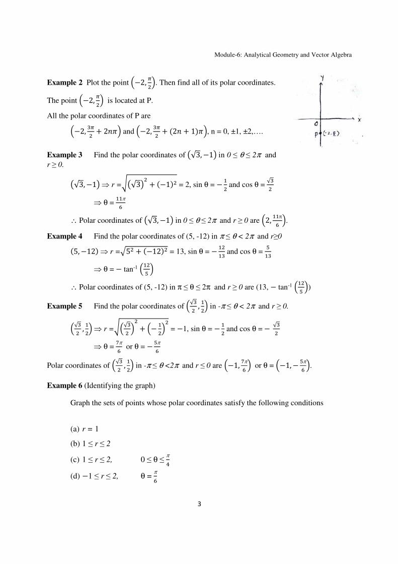
Module-6: Analytical Geometry and Vector Algebra
3
Example 2 Plot the point ?−2, @A. Then find all of its polar coordinates.
The point ?−2, @A is located at P.
All the polar coordinates of P are
?−2, @ + 2-BA and ?−2, @ + 2- + 1BA, n = 0, ±1, ±2,….
Example 3 Find the polar coordinates of C√3, −1E in 0 ≤ θ ≤ 2π and
r ≥ 0.
C√3, −1E ⇒ r =FC√3E + −1 = 2, sin θ = − G and cos θ = √
⇒ θ = GGπH
∴ Polar coordinates of C√3, −1E in 0 ≤ θ ≤ 2π and r ≥ 0 are ?2, GGπH A.
Example 4 Find the polar coordinates of (5, -12) in π ≤ θ < 2π and r≥0
5, −12 ⇒ r =5 + −12 = 13, sin θ = − GG and cos θ = JG
⇒ θ = − tan-1 ?GJ A
∴ Polar coordinates of (5, -12) in π ≤ θ ≤ 2π and r ≥ 0 are (13, − tan-1 ?GJ A)
Example 5 Find the polar coordinates of ?√ , GA in -π ≤ θ < 2π and r ≥ 0.
?√ , GA⇒ r =F?√ A ? G
A = 1, sin θ = G and cos θ =√
⇒ θ = Kπ
H or θ = Jπ
H
Polar coordinates of ?√ , GA in -π ≤ θ <2π and r ≤ 0 are ?1, Kπ
H A or θ = ?1, Jπ
H A.
Example 6 (Identifying the graph)
Graph the sets of points whose polar coordinates satisfy the following conditions
(a) r = 1
(b) 1 ≤ r ≤ 2
(c) 1 ≤ r ≤ 2, 0 ≤ θ ≤ π
! (d) 1 ≤ r ≤ 2, θ =
π
H

Module-6: Analytical Geometry and Vector Algebra
4
(e) r ≤ 0, θ = π
! (f)
π
≤ θ ≤ Jπ
H , r ≥ 0
(g) π
≤ θ ≤ Jπ
H
Note r = a : Circle of radius |(|centred at O
2 2 M Circle of radius 2 centred at O
θ = θ0 : Line through O making an angle θ0 with the initial ray
Question A polar
Representation of x-axis : θ = 0 +ve x-axis : θ = 0 , r > 0.

Module-6: Analytical Geometry and Vector Algebra
5
x= r cos θ
y = r sin θ
Representation of y-axis : θ = π
+ve y-axis : θ =π, r > 0.
In order to represent the points on the plane, now we have two coordinate systems. Let’s
now see their interrelation
Relating Polar and Cartesian coordinates :
If (r, θ) is given we can obtain the x= r cosθ
corresponding cartesian coordinate by y= r cosθ
Question If (x,y) is given, how to obtain the corresponding polar coordinates?
r2 = x2 + y2
↓
Two values of r : + ,
↓
cosθ = N, sinθ =
ON , letting r ≠ 0 [If r = 0 then θ can be any value]
↓
Obtain unique θ ∈ (0, 2π) corresponding to a particular r.
or θ ∈ (π, π)
Example 7 Find the polar coordinates of the point whose cartesian coordinates (-1, 1).
Solution (x,y) = (1, 1)⇒ x =1, y =1
r2 = x2 + y2⇒ r2 = 2 ⇒ r =√2, √2 sin +ve
r =√2 : cosθ = N = G
√, sinθ = ON =
G√ cos -ve
θ =π π! π
! *

Module-6: Analytical Geometry and Vector Algebra
6
∴ A polar coordinates of the cartesian coordinates (1, 1) is ?√2, π4 A
Example 8 Converting cartesian to polar equation
xy – equation → rθ equation
Given (x2)2 + y2 = 4 Use the relation
Solution (r cosθ 2)2 + y27,- = 4 x rcos θy rsin θ
U
⇒ 4r cosθ + 4 = 4
⇒ r ( r 4 cosθ ) = 0
⇒ r = 0 or r = 4 cosθ
⇒ r = 4 cosθ.
Example 9 Converting polar to cartesian coordinate
rθ equation → xy – equation Typeequationhere. (a) r = 1 + 2r cosθ Use the relation
(b) r = 1 cosθ r2 = x2 + y2
cosθ = = N
sinθ = ON
Solution: (a) r = 1+2x ⇒ r2 = (1+2x)2 ⇒ x2+ y2 =1+ 4x + 4x2 ⇒ y23 x2 4x 1 =0
(b) r = 1cosθ ⇒ r2 = r cosθ ⇒ x2+ y2 = r x
⇒ ( x2+ y2 + x )2 = r2
⇒ x4+ y4 + x2+2 x2y2+2 y2x +2x3 = x2 + y2
⇒ x4+ y4 + 2 x2y2+2 xy2 + 2x3y2 = 0
Conic Section in Polar Coordinates
Lines Equation of the line L :
where r0 ≥ 0, P0(r0, θ0) is the foot
of perpendicular from the origin
to the line L.
Don’t use
r =^
r cos(θθ0) = r0

Module-6: Analytical Geometry and Vector Algebra
7
Example 10 Find the equation of the line in which the point ?2, π4 A is the foot of perpendicular
from the origin
r cos?θ @! A = 2
Cartesian r cosθ? G√A 7,-θ ? G
√A = 2
⇒ yx = 2√2
Note Ax + By + C = 0, (A, B) ≠ (0,0)
R (A cosθ +B sinθ ) + C = 0
⇒ r cos(θ θ0 ) = r0
↓
$/√ `
Circle Equation of a circle with centre P0(r0,θ0) and radius a
2r r0 cos (θθ0) = r2+" a2
⇒
Example 11 Find the polar equation of a circle with centre ?1, π2Aand radius 1.
Center : ?1, π2A
Radius : 1
1 = r2 + 1 2r cos ?θ @A
⇒ r = 2 sin θ
Particular cases
Circles passing through origin
a2 = r2+a2 2ra cos(θθ0)
⇒ r =2a cos(θθ0)
a2 = r2+a2 2ra cos(θθ0) x2+ y2 + 2y = 0
⇒ r =2a cos(θθ0) ⇒ x2+ (y+1)2 = 1
Subcases (i) Centre lies on the positive y-axis
θ0 = @
a2 = r2+" 2r r0 cos(θ θ0)

Module-6: Analytical Geometry and Vector Algebra
8
r =2a cos(θ @) = 2a sin θ
(ii) Centre lies on the positive x-axis
θ0 = 0
r =2a cos(θ0)= 2a cos θ
(iii) Centre lies on the negative x-axis
θ0 = π
r =2a cos(θ π)= 2a cos θ
(iv) Centre lies on the negative y- axis
θ0 = @
r =2a cos(θ +@)= 2a sin θ
Conic Sections
abbc = e ⇒
NdNefgθ
= e ⇒ r = e ( k – r cosθ)
⇒ r = dh
Gihefgθ, where x = k > 0 is the vertical directrics
If the directrix is the line x = k, k > 0, i.e. directrics lies on the left of the origin
r = dh
Ghefgθ

Module-6: Analytical Geometry and Vector Algebra
9
If y = k, k > 0, is the directrics
r = dh
Ghgjkθ
If y = k, k > 0, is the directrics
r = dh
Gihgjkθ
Examples 12 (Polar equation of a hyperbola)
Find the polar equation of the hyperbola with
eccentricity e = and directrix x=2
K= > 0, e =
r = dh
Gihefgθ =
Gil efgθ
= H
iefgθ
Example 13 (Finding a directrix)
Find the directrix of a parabola r = J
G"iG"efgθ
r = J/G"Giefgθ
: x = 5/2
*Find the ellipse with eccentricity e and semi-major axis a
k = mh – ae
⇒ ke = a(1 8)
equation r = mGh Gihefgθ
Particular Case
a/e
e = 0 ⇒ r = a : circle

Module-6: Analytical Geometry and Vector Algebra
10
Directional Derivative
Gradient
The gradient vector of a function f(x,y) at a point p0(x0,y0) is the vector
∇<<= |op,qpr O|op,qpt Notation ∇<<=, grad(f)
This is the direction in which functional rate of changes is maximum but the question is how to
measure the rate of changes of a function along any direction. We have already learnt that
functional rate of change along the x-axis & y-axis and are given by first order partial
derivatives. This rate of change of a function along a particular direction is known as directional
derivative.
Q
Directional derivative %u %Gv %w x ;"7G%u
Rate of change of f(x,y) at P0(x0,y0) and along %u is s s≥ 0
Ltz→bzb
|bz<<<<<=| P0
= Ltg→"pig~,Opig p,Opg , this limit (if exists) is called directional
derivative of f at p0 along %u
Notation ?gA.bp or bp Attention! The given direction in the def. is a unit vector.
Example 1 Let f(x,y) = O iO ,, ≠ 0,0
0, 0,0 Find the directional derivative of f(x,y) at (0,0) in the direction of the vector %u ? G
√A v ? G√A w
Solution
Ltg→"?"i
√ ,"i √ A","g
Ltg→"/ √ "
g

Module-6: Analytical Geometry and Vector Algebra
11
Ltg→"g
|g|= 0 along v w is G√
∴ Required directional derivative is 0.
Let's relook the definition of directional derivative for a differentiable function
bp Ltg→"pig~,Opig p,Opg ,
= Ltg→"op,Opg~iqp,Opg i∈~g~i∈ g g 6ℎ88 ∈G →0∈ →0(77→0
= ", "%G O", "%
= C", "v O", "wE. Gv, w = /(b". %u Example 2 Find the directional derivative of the function f(x,y) =2xy 3y2 at P0(5,5) in the
direction = = 4v 3w Solution fx (x,y) =2y, fy(x,y) =2x 6y : both the functions are continuous everywhere
∴ the function is differentiable everywhere
⇒C=Eb" CEb". =|=| = C5,5v O5,5wE. ?!J v
J wA 4
Attention! If the direction is given by (= of any length (≠ 0) then
m<=ρ" ?gAρ" C∇<<=Eρ"m<=|m<=| (f is differentiable function)
Properties of Directional Derivative
∇<<=. %u |∇<<=|. |%u|$.7θ,θ ⟨∇<<=. %u⟩ =|∇<<=|$.7θ
1. When cos θ =1 or θ =0, i.e. %u ∇<<=|∇<<=| then has maximum value. Therefore the
function increases most rapidly along the gradient direction.
The directional derivative along ∇<<= is |∇<<=|.
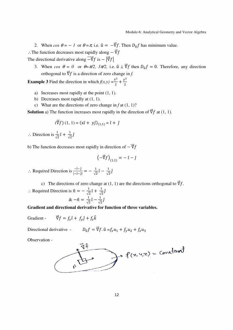
Module-6: Analytical Geometry and Vector Algebra
12
2. When cos θ = 1 or θ =π, i.e. %u ∇<<=. Then has minimum value.
∴The function decreases most rapidly along ∇<<=
The directional derivative along ∇<<<<<= is |∇<<=| 3. When cos θ = 0 or θ=π/2, 3π/2, i.e. %u ∇<<= then 0. Therefore, any direction
orthogonal to ∇<<= is a direction of zero change in f.
Example 3 Find the direction in which f(x,y) = O
a) Increases most rapidly at the point (1, 1).
b) Decreases most rapidly at (1, 1).
c) What are the directions of zero change in f at (1, 1)?
Solution a) The function increases most rapidly in the direction of ∇<<= at (1, 1).
(∇<<=(1, 1) = xv wG,G= v w ∴ Direction is
G√ v G√ w
b) The function decreases most rapidly in direction of ∇<<<=
C∇<<=EG,G v w ∴ Required Direction is
rt|rt| G√ v G√ w
c) The directions of zero change at (1, 1) are the directions orthogonal to ∇<<=. ∴ Required Direction is -u G√ v G√ w & -u G√ v G
√ w Gradient and directional derivative for function of three variables.
Gradient - ∇<<= v Ow 5
Directional derivative - ∇<<=. %u =%G O% %
Observation -

Module-6: Analytical Geometry and Vector Algebra
13
Change of order of integration in triple integral.
Example. Let D be the region bounded by the parabolid # and the plane # 2. write the triple integral to evaluate the vol. of D in the order of # , #, #. Step 1.
Step 2.
Step 3. Eliminate # from # 2 & #
2 0
1 1.
I #O iO
OO OO
O"

Module-6: Analytical Geometry and Vector Algebra
14
Eliminate y from # 2&#
# !
# 4# 0
# 2 2
√ O/√! √! !" #
0, gives
# 0
O O
OO O" #
Here elimination will not work since the projection consists of projections of two surfaces # 2&# where as in the previous two we projected the curve on # 2 itself.
Triple integral in cylindrical & spherical coordinate system: First we shall introduce the
coordinate systems then we will go to find the integral w.r.t those coordinate system.
Let’s suppose you have a point in the 3D space with Cartesian coordinates (, , #). We can also
locate this point in two different mamaers.
Cartesian

Module-6: Analytical Geometry and Vector Algebra
15
Cylindrical
Cylindrical=Polar (, ) in , plane
# Cartesian, B, B or 0, 2B
Spherical
; |0;<<<<<=| ≥ 0
∠C0;<<<<<=, vezaxisE0, B cylindrical, B, B Or 0, 2B cylindrical,
ρsin cos , ρsin sin , # ρ cos
ρ #, unlike r, ρ is always ≥ 0. Volume/ Triple integrals w.r.t three coordinate system:
∭ , , #>c => To evaluate over D⊂ 3 space, where D is a bounded region.
As we have defined triple integral for Cartesian coordinates, we have to discretize the region D
through some elementary regions whose boundaries are given by constant values of the
variables. Well firs then we try to find the surfaces those are given by constant values of the
variables.
Cartesian
( → plane
§ → plane
z = c→ plane > #

Module-6: Analytical Geometry and Vector Algebra
16
Cylindrical
¨ → plane
# 4 → plane
> #
Spherical
". Cone
Constant ∶ plane
> « sin «

Module-6: Analytical Geometry and Vector Algebra
17
Volume elements ¬: Cartesian
> #
Cylindrical
##", #" Δ# ", " Δ ", " Δ
> #
Spherical
Steps, ¯0, 0 Δ° 1g 0, 0 Δ
2k« «"
3N ¯0, 0 Δ°

Module-6: Analytical Geometry and Vector Algebra
18
> « sin«.
Example 1: Find the iterated integral in the order of « to evaluate volume of the solid
bounded below by the plane, on the sides by the 7±ℎ« 2 and above by the cone @.
(Spherical Coordinate)
«²²"³ ∅³l
@µ" sin∅ «∅
Example 2: Find the integral in the cylindrical coordinate system to evaluate volume of the solid, in the
1st hyper octant that is bounded on the side by sin, above by the sphere # 1
#√GN
"
¶jkµ
N"
@
µ"
sin∅ => sin
=
= G G
Example 3: (changing order of integration in cylindrical coordinate)
Let D be the region bounded below by the cone # and above by the paraboloid # 2 . Set up the triple integral in cylindrical coordinates that give the volume of D using the
following order of integration.

Module-6: Analytical Geometry and Vector Algebra
19
(a) # (b)# (c) #
Solution. (a) #
Eliminate; #= # 2 .
? A - 2= 0
? 1A? 2A 0
1.
#N NGN"@µ"
(b) #N"G"@µ"
#√N"G@µ"
(c) #@µ"N NGN"
" , # #"

Module-6: Analytical Geometry and Vector Algebra
20
Example 4: (Changing order of integration in spherical coordinates)
Let D be the region bounded below by the plane# 0, above by the sphere # 4,
and on the sides by the cylinder 1. Set up the triple integrals in spherical coordinates that give
the volume of D using the following orders of integration:
(a) «∅ (b) ∅±
Solution: (a): «²"³·∅"@µ" sin∅ «∅
«efghe∅²"³ ∅³·
@µ" sin ∅ «∅
# 4 1U # √3 ∴ # ≥ 0
* 1# √3
∅ ∠?0, 0, 1, C0, 1, √3EA
=cosG √√G√! =
@H
1
« sin∅ 1
« 4.784∅
(b). «¹º»¼~~½²"²G@µ" sin ∅ ∅«
+ ∅«³ ∅"G²"@µ"
Module-6: Analytical Geometry and Vector Algebra
21
(1) Double & iterated integral / repeated integral , O , O (Fubini’s
Theorem).
(2) Rules in integrations, properties.
Assignment 1
(1) Find Volume of the region bounded above by the surface # 2 and below by the
square|| || 1.
Sol.: Vol 2iGG"G 2GG"G
(2) Evaluate ∬ where r is the region bounded by the lines , 2,& 2.
Sol.: ∬ /" G/ G¿G
(3) Find the volume of the solid cut from the square col. || || ≤ 1 by the planes # 0 &3 # 3.
Sol.: Vol 3 3iGG"G 3 3GGG" 6
(4) Find ∬ √4 where R is the sector cut from the disk ≤ 4 by the rays B 6Â & B 2Â .
Sol.: @H ,
√; ∬ √4 √4 √! √Â√" "√à .
(5) Evaluate the integral tanG B" tanG by converting it to a double integral.
Sol: GGiO
@" GGiO
OO @Â" G
GiO O @Â
@ .
= 2 tanG 2B 2 tanG 2 G@ ln1 4B ÄkJ
(6) A solid right (noncircular) cylinder has its base R in the planeandisbounded above by
the parabolid # . The cylinder’s Volume is

Module-6: Analytical Geometry and Vector Algebra
22
O
"
G
"
O
"
G
Sketch the base and region R and express the cylinder’s Volume as a single iterated integral with order of
integral reversed. Then evaluate the integral.
Sol.: "G" 4/3
(7) Change the order of integration and hence evaluate q!O ! "" & O
OÆiG√l¿"
Sol.: h q!O hÇG
¿!O"¿" ; G
GiOÆ ÄkGK!
Ol""
(8) How would you evaluate the double integration of constant function , over the region R
in the , plane enclosed by the hincye with vertices 0,1, 2, 0, &1, 2;
Sol: , O/OG" , O/OGG

Module-6: Analytical Geometry and Vector Algebra
23
Gradient, Divergence and Curl:
We will start with the concept of Point function:
A variable quantity whose value at any point in the region of the space deptnds upon the positon of the
point, is called a point function.
Types of point functions are
1)- scaler point function:if to the each point P(x,y,z) of region Rin the space there corresponding a
unique scaler f(P), then f is called a scaler point function. We also call it a scalar field. Hence, a scalar
field is a function points in space to points real numbers. For example Temperature distribution in a
heated body, density of a body and the potiential due to gravity are scaler point function or scalar field.
2)-Vector point function: if to each point P(x,y,z) of the region R in the space there corresponds a
unique vector f(P), then f is called a vector point function. This is also called as vector field. Hence,
vector field is a function from points in space to vectors in space. The velocity of a moving fluid,
gravitational force are the examples of the vector point function.
Gradient of a Scaler function:
Definition of gradient:If φ(x,y,z) be a scaler point function then v ÉÉ + w ÉÉO +5 ÉÉ is called the
gradient of the scaler function φ.
It is denoted by grad φ or ∇ φ.
Thus, grad φ = v ÉÉ + w ÉÉO +5 ÉÉ
grad φ =(v ÉÉ + w ÉÉO +5 ÉÉ ) φ(x,y,z)
grad φ = ∇ φ
Hence, We recognize the gradient as the generalization of the derivative.
Remark:From Vector Calculus we know that the partial derivatives , ,f f f
x y z
∂ ∂ ∂
∂ ∂ ∂
give the rates of change of f(x, y, z) in the directions of , , ,i j krr r
respectively. Hence, if the
gradient of t at a point P is not zero, i.e., ( ) ( ) 0,f P Grad f P∇ = ≠r
then it is a vector in the direction
of maximum increase of f at P.
Properties of gradient
(i) Gradient of a scalar quantity is a Vector quantity.

Module-6: Analytical Geometry and Vector Algebra
24
(ii) Magnitude of that vector quantity is equal to the Maximum rate of change of that scalar
quantity.
(iii) Change of scalar quantity does not depend only on the coordinate of the point, but also on
the direction along which the change is shown.
Geometrical meaning of the Gradient
As we know that a surface is all points in 3( , , )x y z ∈ that verifies ( , , ) ,f x y z c= for some smooth
scalar field f and constant c.
Example: Consider the unit sphere in 3 , 2
:S
2 3 2 2 2( , , ) : 1 .S x y z x y z= ∈ + + =
From the following, we can understand the geometrical meaning of gradient:
Definition of level surface:If a surface φ(x,y,z) =c passes through a point and the value of the
function at each point of the surface is the same as at P, then such a surface is called a level
surface through P. For example, if φ(x,y,z) is represents potiential at the point P,then
equipotential surface φ(x,y,z)=c is a level surface.Two level surface cannot intersect.
Let a level surfce pass through the point P at which the value of the function is φ. Consider
another level surface passing through Q,where the value of the function is φ+dφ.
Let and+δ be the position vector of P an Q then ;x<<<<<== δ
∇ φ.d= (v ÉÉ + w ÉÉO +5 ÉÉ ). (v dx + wdy +5 dz )
=ÉφÉdx+
ÉφO dy+
ÉφÉ dz =dφ ….. ………………..(1)
If Q lies on the level surface of P, then dφ=0
Equation (1) beecomes ∇ φ.d=0. Then ∇ φ is to d (tangent).
Hence, ∇ φ is normal to the surface φ(x,y,z)=c.
Let ∇ φ =|∇ φ|ÌÍ ,where ÌÍ is a unit normal veator. Let Î- be the perpendicular distance between two
level surface through P and R. then the rate of change of φ in the direction of the normal to the
surface through P is ÉφÉk .
φk = limÐk→" ÉφÉk = limÐk→" ∇Ñ.dÉk
= limÐk→" |∇Ñ|ÒÍ.dÉk

Module-6: Analytical Geometry and Vector Algebra
25
= limÐk→" |∇Ñ|δn Ék =|∇φ|
|∇ φ| = ÉφÉk.
Hence, gradient φ is a vector normat to the surface φ =c and has a magnitude equal to the rate of
change of φ along this normal. Hence, we have the following theorem as geometrical
interpritation of gradient:
Theorem: Let f be differentiable and S = 3( , , ) : ( , , )S x y z f x y z c= ∈ = be a surface. Then the
gradient of f, f∇ at a point P of the surface S is a normal vector to S at P (provided ( ) 0f P∇ ≠ ).
Engineers use the gradient vector in many physical laws such as:
1. Electric Field (E) and Electric Potential (V): E=-Grad.V
2. Heat Flow (q) and Temperature (T): q(x,y,z)=-kGradT(x,y,z), k is constant
3. Force Field (F) and Potential Energy (U): F(x,y,z)=-GRadU(x,y,z)
Divergence of a Vector function:
The divergence of a vector point function+ is denoted by div F and is defined as below.
Let += =+Gv + +w + +5
Div =+= =∇<<=.+=
= (v ÉÉ + w ÉÉO +5 ÉÉ ).(+Gv + +w + +5)
=Éa~É +
Éa ÉO +ÉalÉ .
It is evident that div += is scaler function.
Physical Intuition
• Divergence (div) is “flux density”—the amount of flux entering or leaving a point. We
can think of it as the rate of flux expansion (positive divergence) or flux contraction
(negative divergence).
• So, divergence is just the net flux per unit volume, or “flux density”, just like regular
density is mass per unit volume (of course, we don’t know about “negative” density).
Imagine a tiny cube—flux can be coming in on some sides, leaving on others, and we
combine all effects to figure out if the total flux is entering or leaving.
• The bigger the flux density (positive or negative), the stronger the flux source or sink. A
div of zero means there’s no net flux change in side the region. i.e.,

Module-6: Analytical Geometry and Vector Algebra
26
• Imagine a fluid, with the vector field representing the velocity of the fluid at each point in space.
Divergence measures the net flow of fluid out of (i.e., diverging from) a given point. If fluid is
instead flowing into that point, the divergence will be negative.
A point or region with positive divergence is often referred to as a "source" (of fluid, or whatever
the field is describing), while a point or region with negative divergence is a "sink".
Geometrical Interpretation of Divergence:
Let us consider the case of a fluid flow. Consider aSmall rectangle pallellopiped of dimension dx,dy,dz
parallel to x,y and z axes resprctively.
Let Ô<= =Ôv + ÔOw + Ô5 be the velocity of the fluid at P(x,y,z).
Mass of the fluid flowing in through the face ABCD in unit time
=Velocity ×Aear of the face
=Ô(dy dz)
Mass of the fluid flowing out across the face PQRS in unit time
= Ô(x+dx)(dy dz)
=(Ô+ ÉÕoÉ dx)(dy dz)
Net decrease in mass of fluid in the parallelopiped corresponding to the flow along x-axis per unit time
= Ô(dy dz)- (Ô+ ÉÕoÉ dx)(dy dz)
=- ÉÕoÉ dxdy dz (minus sign shows decrease)
Similarly, the decrease in mass of fluid to the flow y-axis = ÉÕqÉO dx dy dz

Module-6: Analytical Geometry and Vector Algebra
27
And the decrease in mass of fluid to the flow z-axis = ÉÕÖÉ dx dy dz
Total decrease of the amount of the fluid per unit time =(ÉÕoÉ +ÉÕqÉO +
ÉÕÖÉ ) dx dy dz
Thus the rate of the loss of fluid per unit volume = ÉÕoÉ +ÉÕqÉO +
ÉÕÖÉ =(v ÉÉ + w ÉÉO +5 ÉÉ ).(Ôv + ÔOw + Ô5)
= ∇×.Ô =div Ô .
Remark:If the fluid is incompressible, there can be no gain or no loss in the fluid in the volume element.
Hence
div Ô= 0 ………………………(1)
and V is called a solenoidal vector function.
Equation (1) is also called the equation of the continuity or conservation of mass.
CURL of a Vector
The curl of a vector point function s definrd as below
Curl × += =∇<<= × +=
=?v ÉÉ + w ÉÉO + 5 ÉÉA × (+Gv + +w + +5)
= Ù vÉÉ+GwÉÉO+
5É É+Ù =vÉalÉO -
Éa É ) - wÉalÉ -Éa~É ) + 5Éa É -
Éa~ÉO )
Curl += is the vector quantity.
Physical Meaning of the CURL:
As we know that Ô<= =Ú<<= × =, where Ú is the angular velocity, Ô<= is the linear velocity and = is the position
vector of a point on the rotating body.
Curl Ô<= = ∇<<= × Ô<=
Module-6: Analytical Geometry and Vector Algebra
28
= ∇<<= × (Ú<<= × =) = ∇<<= ×[(ÚGv + Úw+ Ú5 ) × (x v + y w + z 5) ]
= ∇<<= × Û vÚGwÚ
5Ú# Û = ∇<<= ×[(Ú # -Ú y) v +( ÚG z -Ú x) w+( ÚGy -Ú x) 5]
= ?v ÉÉ + w ÉÉO + 5 ÉÉA × [(Ú # -Ú y) v +( ÚG z -Ú x) w+( ÚGy -Ú x) 5]
= Ù vÉÉÚ # − Ú ywÉÉO ÚG z − Ú x
5É É ÚGy − Ú xÙ
=(ÚG+Ú)v – (-Ú − Ú)w + (Ú + Ú)5
= 2(ÚGv + Úw+ Ú5 ) = 2 Ú.
Remark:Curl Ô<= = 2 Ú which shows the curl of a vector field is connected with the rotational properties of
the vector field and the justifies the name rotation used for curl.
If Curl Ô<==0, the field is termed as irrotational.
Lemma -1: Gradient fields are irrotationals. That is, if ,F f= ∇
for some smoothscalar field f, then curl F = 0.
Similarly, some identites related to curl, divergence and Gradient:
for vectors functions , a and b, and scaler functions U are given below:
i)- div curl = Ü . Ü ×a =0
ii)- Ü . Ýa = (Ü Ý)a + U( Ü. a)
= (grad U)a +U(div a)
iii)- Ü ×Ua= UÜ ×a +(Ü Ý) × a
iv)- div a × b = (curl a).b - a.(curl b)
v)- curl a × b =Ü ×( a × b)
=(Ü. b)a –(Ü. a)b + [b .Ü ] a - [a .Ü ] b
Where [a .Ü ] = ?Þ ßß + Þ ßß + Þ ßßA
vi)- curl (curl a) = grad (div a) - Üà a
Module-6: Analytical Geometry and Vector Algebra
29
where Üà a = ÜàÞ+ ÜàÞ+ ÜàÞ
Assignment 2
1)- If =(x v + y w + z 5) then show that
i)- grad r =N ii)- grad(
GN) = áâ
2) if u= x+y+z, v=x2+ y2 +z2, w=yz +zx+xy prove that the grad u, grad v, grad w are coplanar vectors.
3) if u= x2+ y2 +z2, and = =(x v + y w + z 5), then find div (u =) in terms of u.
4) find the value of n for which the vector rn= is solenoidal, where = =(x v + y w + z 5).
5) show that div (grad rn) =n (n+1) rn-2, where = =(x v + y w + z 5).
Hence show that, ∆2 ( G N ) = 0.
6) find the divergence and curl of >= (x y z) v + (3 x2 y) w + (x z2 –y2 z) 5 at (2,-1,1).
7) Prove that (y2 - z2 +3xyz -2x) v + (3xz +2xy) w + (3xy –2xz +2z) 5 is both solenoidal and irrotational.
8) +==(x2 – y2 + x ) v - (2xy + y)w. Is this field is irrotational ? if so, find its scaler potiential.
9) Prove that, the vactor field +==|áâ| is irrotational as well as solenoidal. Find the scaler potential.
10) For a solenoidal vector +=, show that
curl (curl ( curl +=) ) ) = ∇4+= .
11. The gravitational field pr
is the force between two particles at points 0 0 0 0( , , )P x y z= and ( , , )P x y z= .
It is defined by
0 0 03 3[ , , ],
c cp r x x y y z z
r r= − = − − − −
r r
where 2 2 2
0 0 0( ) ( ) ( )r x x y y z z= − + − + −r
and it is irrotational field as the scalar field ( , , )c
f x y zr
= is
a potential for it. Verify it.

Module-6: Analytical Geometry and Vector Algebra
30
Surface Area
of a closed and bounded region on the surface
of ä, , = å with the help of projection on a plane
We often come across to deal with some surfaces that are presented by , , # 4 , a constant, for instance, the equipotential surfaces in the gravitational or electrical or magnetic fields.
In this lecture we intend to evaluate the surface area of a closed and bounded region on
the surface of , , # 4. In due course we shall project the surface under consideration on a
flat region or plane.
Let this plane be R and ± be the unit normal on R. We assume that
(i) The surface is smooth; if not entirely, at least the patch of the surface that we consider
to evaluate the area is smooth. Let this patch be S. Mathematically, this condition
presumes that on S, the function f is differentiable and æ<= is nonnull and continuous.
(ii) When we take perpendicular projection of S on R, we never observe that the surface
folds back over itself. Mathematically, æ<=. ± 0 on S.

Module-6: Analytical Geometry and Vector Algebra
31
Fig : A surface and its projection on R-plane.
We approximate the area of the infinitesimal surface by the tangent surface at p.
As æ<= is perpendicular to the tangent plane æ<= ,7 ±((&&8& 3. %<= × >= ,
when %<= is tangent to the curve PWQ and >= is tangent to the curve PTN.
The value |%<= >=| measures area of the rhombus whose sides are %<= & >=. Here we let
∆σ = |%<= × >=| .
As %<= × >= has the direction perpendicular to the rhombus, the dot product |%<= × >=|. ±
measures area of the region perpendicular to ±.
Hence ∆A = ||%<= × >=. ±|| (absolute value of mod of |%<= × >=|. ±)
= ||%<= × >=| | ±| 4.7 |, r = < ( ±, æ<=)
= ∆P |4.7 |
⇒ ∆P = ∆
|efg N| (cos r ≠0, due to assumption (ii) )
As we approximate ∆σ by the value of ∆P,
∆σ ≈ ∆P= ∆
|çfg N| Since r = < ±, æ<= , above ⇒ |æ<=. ±| = |æ<=| $.7
⇒ 4.7 = |è<<= . éu||è<<=|
Therefore ∆σ = ∆|è<<=||è<<= . éu|
Hence the required surface area =∬ |è<<=||è<<= . éu|
±.ê843,.- .-ë ±&(-8 8/,.-
Surface integrals
If S be the shadow region of a smooth surface Ω, defined by , , # = 4 on the plane
R whose unit normal is ±, and g be a continuous function over the surface Ω, then the integral of
g over Ω, is the integral
∬ /Ω
ì = ∬ /, , #¶ |è<<=||è<<= . éu|
Here we assume that R be such a plane that æ<=. ± 0.
PROPERTY
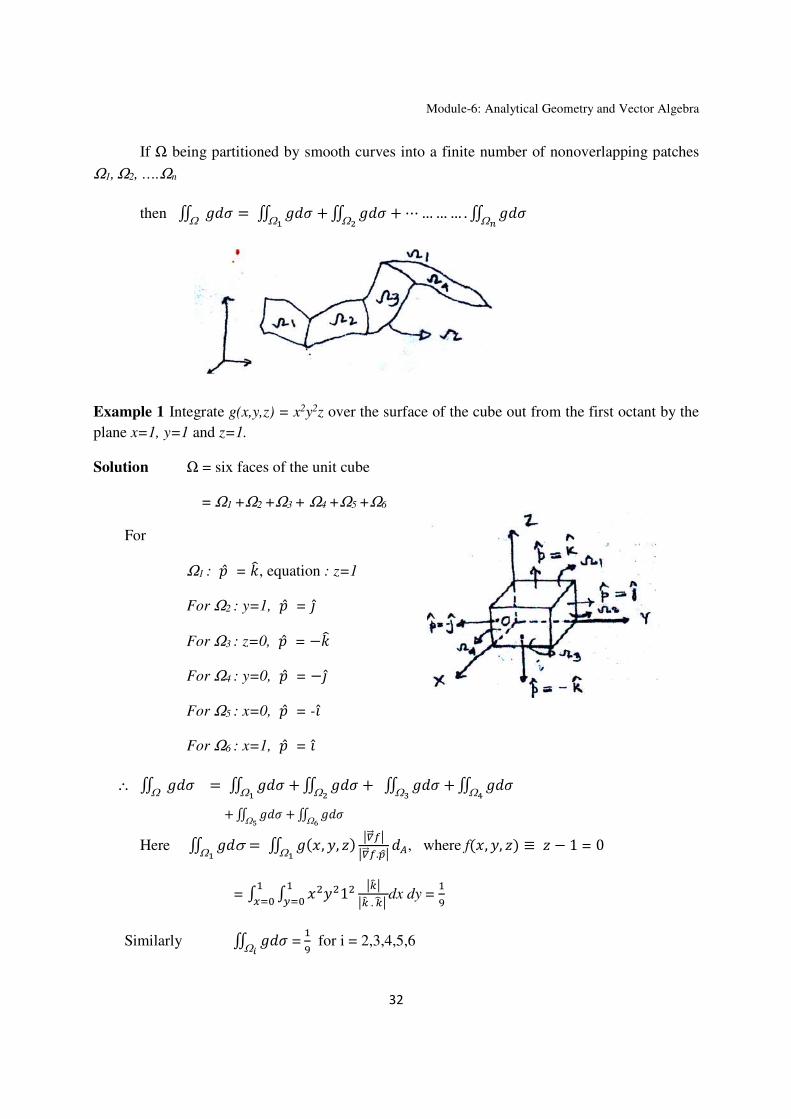
Module-6: Analytical Geometry and Vector Algebra
32
If Ω being partitioned by smooth curves into a finite number of nonoverlapping patches
Ω1, Ω2, ….Ωn
then ∬ /ìΩ
= ∬ /ì +Ω~ ∬ /ì + ⋯ … … … . ∬ /ì
ΩïΩ
Example 1 Integrate g(x,y,z) = x2y2z over the surface of the cube out from the first octant by the
plane x=1, y=1 and z=1.
Solution Ω = six faces of the unit cube
= Ω1 +Ω2 +Ω3 + Ω4 +Ω5 +Ω6
For
Ω1 : ± = 5, equation : z=1
For Ω2 : y=1, ± = w For Ω3 : z=0, ± = −5
For Ω4 : y=0, ± = −w For Ω5 : x=0, ± = -v For Ω6 : x=1, ± = v
∴ ∬ /ìΩ
= ∬ /ì +Ω~ ∬ /ì + ∬ /ì +
Ωl ∬ /ìΩÆΩ
+ ∬ /ì +Ωð ∬ /ì
Ω·
Here ∬ /σΩ~ = ∬ /, , #
Ω~|è<<=||è<<=.éu| , where f, , # ≡ # − 1 = 0
= 1GO"G" |d ||d . dÍ | dx dy =
GÃ
Similarly ∬ /ìΩò = GÃ for i = 2,3,4,5,6

Module-6: Analytical Geometry and Vector Algebra
33
∴ ∬ /ì Ω
= HÃ = .
Example 2 Find the surface area of the surface cut from the cylinder y2 + z2 =1,
z ≥ 0 by the planes x = 0 and x = 1.
Solution The required surface area
= ∬ ìΩ
, Ω ∶ * + # = 1, # ≥ 00≤ ≤ 1
= ∬ |è<<=||è<<=. éu| ¶ ,
where , , # = y2 + z2-1 = 0,
z ≥ 0 & ± = 5
= |Otid ||COtid E.d |GOGG" dxdy
= O i ||GOGG" dxdy
Mathematically this
= ó GGO
GOG ôG" dx shadow region is
= 7,-GGGG" dx õ: * 0≤ ≤ 11≤ ≤ 1
= 2 sin-1 1 sq. unit
References
1. Apostol, T., Mathematical Analysis, Addison-Wesley, 2nd Edition, 1974
2. Thomas, George Brinton, Maurice D. Weir, Joel Hass, and Frank R. Giordano.
Thomas' calculus. Addison-Wesley, 2005.
3. Kreyszig, Erwin, Advanced engineering mathematics, 12th Edition, Wiley.
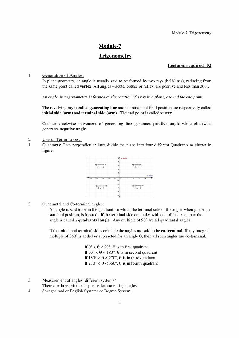
Module-7: Trigonometry
1
Module-7
Trigonometry
Lectures required -02
1. Generation of Angles:
In plane geometry, an angle is usually said to be formed by two rays (half-lines), radiating from
the same point called vertex. All angles – acute, obtuse or reflex, are positive and less than 360°.
An angle, in trigonometry, is formed by the rotation of a ray in a plane, around the end point.
The revolving ray is called generating line and its initial and final position are respectively called
initial side (arm) and terminal side (arm). The end point is called vertex.
Counter clockwise movement of generating line generates positive angle while clockwise
generates negative angle.
2. Useful Terminology:
1. Quadrants: Two perpendicular lines divide the plane into four different Quadrants as shown in
figure.
2. Quadrantal and Co-terminal angles:
An angle is said to be in the quadrant, in which the terminal side of the angle, when placed in
standard position, is located. If the terminal side coincides with one of the axes, then the
angle is called a quadrantal angle. Any multiple of 90° are all quadrantal angles.
If the initial and terminal sides coincide the angles are said to be co-terminal. If any integral
multiple of 360° is added or subtracted for an angle Ɵ, then all such angles are co-terminal.
If 0° < Ɵ < 90°, Ɵ is in first quadrant
If 90° < Ɵ < 180°, Ɵ is in second quadrant
If 180° < Ɵ < 270°, Ɵ is in third quadrant
If 270° < Ɵ < 360°, Ɵ is in fourth quadrant
3. Measurement of angles: different systems°
There are three principal systems for measuring angles:
4. Sexagesimal or English Systems or Degree System:

Module-7: Trigonometry
2
Most commonly used system of measuring angle.
5. Circular System or Radian Measure (or system):
In advanced mathematics, the most convenient system for the measurement of angles is the
circular or radian measures.
1. Definition of π:
For any circle, the ratio of the circumference to its diameter is the same, i.e., this ratio
is independent of the size of the circle.
circumferenceofcircle
diameterofcircle
2. Numerical value of :
Approximate value is 22/7. This is correct to 2 decimal places. The fraction 355/113
is correct to 6 decimal places. Approximate value of π, correct upto 10 decimal
places, is 3.1415926536.
A radian is the measure of an angle at the center of a circle subtended by an arc equal in length to
the radius of the circle.
Radian is a constant angle. One radian = °
One radian is denoted by 1. Thus stands for π radian. Generally, π radian is just denoted by
π.
180° = π, 90° =
, 45° =
, 60° =
, etc.
1 radian = °
= 180° x 0.31831 = 57.2958° = 57° 17’ 44.81’’ approx. = 206265 seconds
approx.
3. Relation between three systems:
For the same angle let the measure be D in degree, G in grades and C in radian.
180° = π radians.
D degrees =
radian …. (i)
100 grades = 1 right angle = 90° =

Module-7: Trigonometry
3
1 grade =
radian, G grades =
….(ii)
From equation (i) and (ii),
=
= C
Hence, !
" =
#
=
$%
Magnitudeofangleincircularmeasure )*+,-./01/22*34/+56+,721
275683
Ɵ )
:
Examples:
Q1) Express 73°25’30’’ in centesimal measure.
Solution: 25’30’’ = ;.;°
= = 0.425°,
Hence, 73° 25’30’’ = 73.425° = >.;°
" rt angles = 81.5833B = 81B 58’33’’
Q2) The angles of a triangle are in AP and the ratio of number of radian in the greatest angle is to the
number of degree in the least one as π : 60. Find the angles in degree.
Solution: Let the number of degree in the angle be A-B, A, A+B, then A= 60°
Again the greatest angle = (A+B)° = (A+B) *
The least angle = (A-B)°
Hence,
(DEF)H
IJK =
=
A+B = 3(A-B), A= 2B
B= 30°. Hence, 30°, 60° and 90°.
TRIGNOMETRICAL RATIO and FUNCTION
A class of real functions defined in terms of ratios of sides of a right angled triangle are known as
trigonometrical function. Sign of trigonometrical ratios of an angle with reference to a right angled
triangle will depend on the quadrant in which the terminal side is located.

Module-7: Trigonometry
4
Some Basic Identities:
1. Definition of Trigonometrical Function unit Circle:
The trigonometrical ratio can be represented through a unit circle.
Take any point on the circle at a arc length of Ɵ.
∟DOB = = L
M =
Ɵ = Ɵ(in radian)
OD = 1, OA = x , AD = y.
sinƟ = NO
PQ =
R
= y
cosƟ = PQ
P =
S
= x
tanƟ = R
S , cotƟ =
S
R , cosecƟ =
R and secƟ =
S
From the diagram, x2 + y2 = 1, all equation in section 1 can be derived from this.
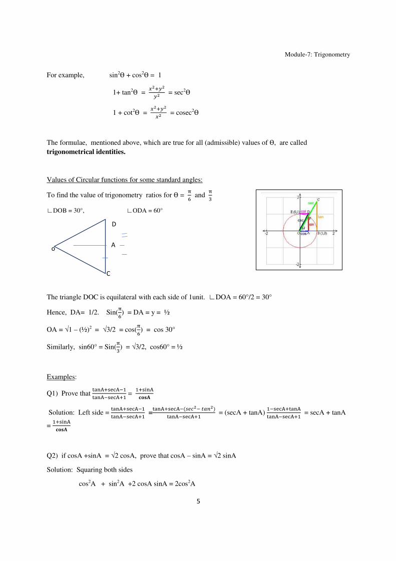
Module-7: Trigonometry
5
For example, sin2Ɵ + cos2
Ɵ = 1
1+ tan2Ɵ =
TUVWU
WU = sec2
Ɵ
1 + cot2Ɵ =
TUVWU
TU = cosec2
Ɵ
The formulae, mentioned above, which are true for all (admissible) values of Ɵ, are called
trigonometrical identities.
Values of Circular functions for some standard angles:
To find the value of trigonometry ratios for Ɵ =
X and
∟DOB = 30°, ∟ODA = 60°
The triangle DOC is equilateral with each side of 1unit. ∟DOA = 60°/2 = 30°
Hence, DA= 1/2. Sin(
X) = DA = y = ½
OA = √1 – (½)2 = √3/2 = cos(
X) = cos 30°
Similarly, sin60° = Sin(
) = √3/2, cos60° = ½
Examples:
Q1) Prove that YZ[QV\]^QJ
YZ[QJ\]^QV =
V\_[Q
1/3I
Solution: Left side = YZ[QV\]^QJ
YZ[QJ\]^QV =
YZ[QV\]^QJ(`aUJbcdU)
YZ[QJ\]^QV = (secA + tanA)
J\]^QVYZ[Q
YZ[QJ\]^QV = secA + tanA
= V\_[Q
1/3I
Q2) if cosA +sinA = √2 cosA, prove that cosA – sinA = √2 sinA
Solution: Squaring both sides
cos2A + sin2A +2 cosA sinA = 2cos2A
C
o
A
D
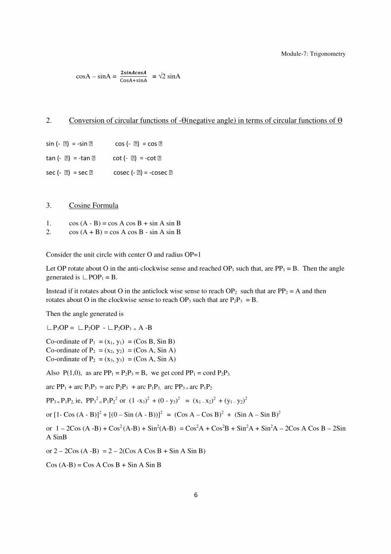
Module-7: Trigonometry
6
cosA – sinA = $efghijeh
kl\QV\_[Q = √2 sinA
2. Conversion of circular functions of -Ɵ(negative angle) in terms of circular functions of Ɵ
sin (- Ɵ) = -sin Ɵ cos (- Ɵ) = cos Ɵ
tan (- Ɵ) = -tan Ɵ cot (- Ɵ) = -cot Ɵ
sec (- Ɵ) = sec Ɵ cosec (- Ɵ) = -cosec Ɵ
3. Cosine Formula
1. cos (A - B) = cos A cos B + sin A sin B
2. cos (A + B) = cos A cos B - sin A sin B
Consider the unit circle with center O and radius OP=1
Let OP rotate about O in the anti-clockwise sense and reached OP1 such that, are PP1 = B. Then the angle
generated is ∟POP1 = B.
Instead if it rotates about O in the anticlock wise sense to reach OP2 such that are PP2 = A and then
rotates about O in the clockwise sense to reach OP3 such that are P2P3 = B.
Then the angle generated is
∟P3OP = ∟P2OP - ∟P2OP3 = A -B
Co-ordinate of P1 = (x1, y1) = (Cos B, Sin B)
Co-ordinate of P2 = (x2, y2) = (Cos A, Sin A)
Co-ordinate of P2 = (x3, y3) = (Cos A, Sin A)
Also P(1,0), as are PP1 = P2P3 = B, we get cord PP1 = cord P2P3.
arc PP1 + arc P1P3 = arc P2P3 + arc P1P3, arc PP3 = arc P1P2
PP3 = P1P2, ie, PP32 = P1P2
2 or (1 -x3)2 + (0 - y3)
2 = (x1 – x2)2 + (y1 – y2)
2
or [1- Cos (A - B)]2 + [(0 – Sin (A - B))]2 = (Cos A – Cos B)2 + (Sin A – Sin B)2
or 1 – 2Cos (A -B) + Cos2 (A-B) + Sin2(A-B) = Cos2A + Cos2B + Sin2A + Sin2A – 2Cos A Cos B – 2Sin
A SinB
or 2 – 2Cos (A -B) = 2 – 2(Cos A Cos B + Sin A Sin B)
Cos (A-B) = Cos A Cos B + Sin A Sin B
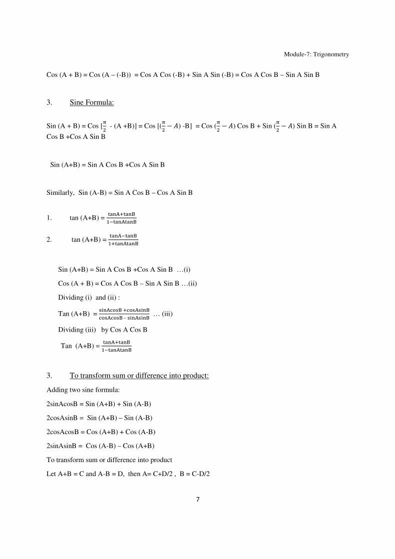
Module-7: Trigonometry
7
Cos (A + B) = Cos (A – (-B)) = Cos A Cos (-B) + Sin A Sin (-B) = Cos A Cos B – Sin A Sin B
3. Sine Formula:
Sin (A + B) = Cos [
- (A +B)] = Cos [(
− n) -B] = Cos (
−n) Cos B + Sin (
− n) Sin B = Sin A
Cos B +Cos A Sin B
Sin (A+B) = Sin A Cos B +Cos A Sin B
Similarly, Sin (A-B) = Sin A Cos B – Cos A Sin B
1. tan (A+B) = YZ[QVYZ[o
JYZ[QYZ[o
2. tan (A+B) = YZ[QJYZ[o
VYZ[QYZ[o
Sin (A+B) = Sin A Cos B +Cos A Sin B …(i)
Cos (A + B) = Cos A Cos B – Sin A Sin B …(ii)
Dividing (i) and (ii) :
Tan (A+B) = \_[Q^l\o V^l\Q\_[o^l\Q^l\o – \_[Q\_[o … (iii)
Dividing (iii) by Cos A Cos B
Tan (A+B) = YZ[QVYZ[o
JYZ[QYZ[o
3. To transform sum or difference into product:
Adding two sine formula:
2sinAcosB = Sin (A+B) + Sin (A-B)
2cosAsinB = Sin (A+B) – Sin (A-B)
2cosAcosB = Cos (A+B) + Cos (A-B)
2sinAsinB = Cos (A-B) – Cos (A+B)
To transform sum or difference into product
Let A+B = C and A-B = D, then A= C+D/2 , B = C-D/2

Module-7: Trigonometry
8
Replacing these values in 1, 2, 3 and 4 above
Sin C + Sin D = 2 Sin (kV
) Cos (kJ
)
Sin C – Sin D = 2 Cos (kV
) Sin (kJ
)
Cos C + Cos D = 2 Cos (kV
) Cos (kJ
)
Cos C – Cos D = 2 Sin (kV
) Sin (Jk
)
4. Graph of trigonometry ratio:
Examples:
Q1) Prove that, YZ[ CQVoGVYZ[ CQJoG
JYZ[ CQJoGYZ[ CQVoG = tan2A
Solution: Let A+B = C and A-B = D
Left side YZ[ kVYZ[
JYZ[ kYZ[ = tan(C+D) = tan (A+B +A -B) = tan2A
Q2) If A+B+C = π and cos A = cos B.cosC, Prove that
tanA = tanB+tanC
Solution: Right side = tan B + tanC =\_[o^l\o +
\_[k^l\k =
\_[o^l\kV\_[k^l\o^l\o^l\k =
\_[ CoVkG^l\Q =
\_[ CJoG^l\Q =
tanA
Formulae on multiple angles :

Module-7: Trigonometry
9
Question 1 sin (A + B) = sin A cos B + cos A sin B
Taking B = A, we get
sin 2A = 2 sin A cos A
= 2 \_[ Q^l\ Q cos2A
= YZ[ Q\]^UQ = =
YZ[ QVYZ[UQ
Question 2 cos (A + B) = cos A cos B - sin A sin B
taking B = A, we get
cos 2A = cos2A - sin2A
= cos2A-(1- cos2A) = (1- sin2A) - sin2A
= 2 cos2A-1 = 1- 2sin2A
= cos2Aq1 − \_[UQ^l\UQr
= JYZ[U QVYZ[UQ
Question 3 tan 2A = \_[ Q^l\ Q =
YZ[ QJYZ[UQ
Formulae on submultiple angles:
Again considering 2A = θ, we get the following formulae for submultiple angles
sin θ = 2 sin θ
cos θ
= YZ[ θU
VYZ[UθU
cos θ = cos θ
− sin θ
= 2 cos θ
− 1
= 1−2 sin θ
= JYZ[Uθ
UVYZ[Uθ
U
tan θ = YZ[ θU
VYZ[UθU
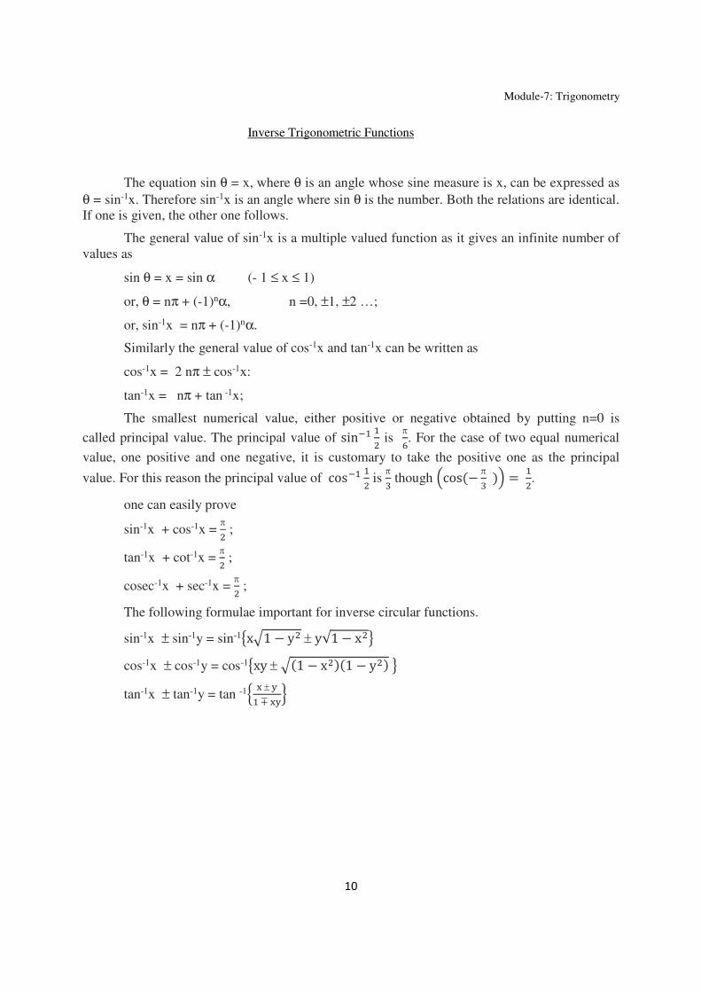
Module-7: Trigonometry
10
Inverse Trigonometric Functions
The equation sin θ = x, where θ is an angle whose sine measure is x, can be expressed as
θ = sin-1x. Therefore sin-1x is an angle where sin θ is the number. Both the relations are identical.
If one is given, the other one follows.
The general value of sin-1x is a multiple valued function as it gives an infinite number of
values as
sin θ = x = sin α (- 1 ≤ x ≤ 1)
or, θ = nπ + (-1)nα, n =0, ±1, ±2 …;
or, sin-1x = nπ + (-1)nα.
Similarly the general value of cos-1x and tan-1x can be written as
cos-1x = 2 nπ ± cos-1x:
tan-1x = nπ + tan -1x;
The smallest numerical value, either positive or negative obtained by putting n=0 is
called principal value. The principal value of sinJ is
π
X. For the case of two equal numerical
value, one positive and one negative, it is customary to take the positive one as the principal
value. For this reason the principal value of cosJ is
π
though qcos C− π
Gr = .
one can easily prove
sin-1x + cos-1x = π
;
tan-1x + cot-1x = π
;
cosec-1x + sec-1x = π
;
The following formulae important for inverse circular functions.
sin-1x ± sin-1y = sin-1txv1 − y ± y√1 − xy
cos-1x ± cos-1y = cos-1txy ± vC1 − xGC1 − yG y
tan-1x ± tan-1y = tan -1z S ± R ∓ SR|
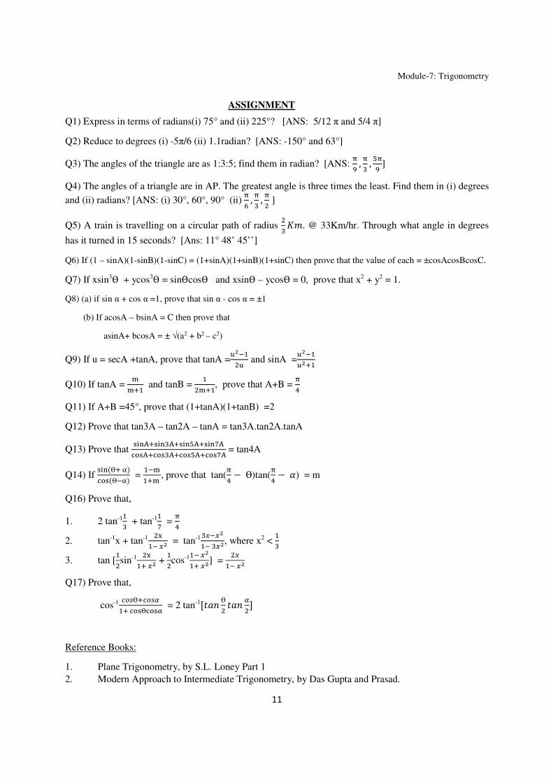
Module-7: Trigonometry
11
ASSIGNMENT
Q1) Express in terms of radians(i) 75° and (ii) 225°? [ANS: 5/12 π and 5/4 π]
Q2) Reduce to degrees (i) -5π/6 (ii) 1.1radian? [ANS: -150° and 63°]
Q3) The angles of the triangle are as 1:3:5; find them in radian? [ANS: ,
, ; ]
Q4) The angles of a triangle are in AP. The greatest angle is three times the least. Find them in (i) degrees
and (ii) radians? [ANS: (i) 30°, 60°, 90° (ii) X , ,
]
Q5) A train is travelling on a circular path of radius . @ 33Km/hr. Through what angle in degrees
has it turned in 15 seconds? [Ans: 11° 48’ 45’’]
Q6) If (1 – sinA)(1-sinB)(1-sinC) = (1+sinA)(1+sinB)(1+sinC) then prove that the value of each = ±cosAcosBcosC.
Q7) If xsin3Ɵ + ycos3
Ɵ = sinƟcosƟ and xsinƟ – ycosƟ = 0, prove that x2 + y2 = 1.
Q8) (a) if sin α + cos α =1, prove that sin α - cos α = ±1
(b) If acosA – bsinA = C then prove that
asinA+ bcosA = ± √(a2 + b2 – c2)
Q9) If u = secA +tanA, prove that tanA =UJ
and sinA =
UJ
UV
Q10) If tanA =
V and tanB =
V, prove that A+B =
Q11) If A+B =45°, prove that (1+tanA)(1+tanB) =2
Q12) Prove that tan3A – tan2A – tanA = tan3A.tan2A.tanA
Q13) Prove that \_[QV\_[QV\_[;QV\_[>Q
^l\QV^l\QV^l\;QV^l\>Q = tan4A
Q14) If \_[ CƟV G^l\ CƟJ) =
J
V , prove that tan( − Ɵ)tan(
− ) = m
Q16) Prove that,
1. 2 tan-1 + tan-1
> =
2. tan-1x + tan-1 SJ TU = tan-1TJTU
J TU, where x2 <
3. tan [sin-1 S
V TU + cos-1J TU
V TU] = T
J TU
Q17) Prove that,
cos-1 `ƟV`V ^l\Ɵ^l\ = 2 tan-1[
Ɵ
]
Reference Books:
1. Plane Trigonometry, by S.L. Loney Part 1
2. Modern Approach to Intermediate Trigonometry, by Das Gupta and Prasad.

Module-8: Probability
1
Module-8
Probability
Lectures required -02
Probability theory deals with the rules governing the chances of occurrence of
phenomena, which are random in nature. To introduce probability, certain basic terms are
needed, we first discuss those terms.
Random experiment:
A random experiment is an experiment which can be repeated under identical
conditions, the set of all possible outcomes is known but before any particular performance of
the experiment, we cannot predict which outcome will occur. For example, tossing of a coin,
rolling of a die etc. Any particular performance of a random experiment is called a trial.
Sample space:
The set S of all possible outcomes of a random experiment is called the sample space
associated with that random experiment. For example, in tossing of a coin, = , where H
and T resp. denote getting a head and tail. In rolling of a die, = , , , , , where
denotes the outcome in which appears at the uppermost face, = 1, 2, 3, 4, 5, 6 .
Event:
An event in a random experiment is defined as any subset of the sample space S.
Singleton subsets are called elementary events, ∅ is called the impossible event and S is called
the certain event, e.g., in rolling of a die , , is an event which is precisely ‘getting an
odd number’.
If for any two events A and B, ∈ ∪ we say that at least one of the events A or B
occurs. If ∈ ∩ , then we say that both A and B have occurred. If ∉ , then we say that
the complementary event ′ has occurred.
Favourable outcomes to an event:
An outcome is said to be favourable to an event A if it entails the happening of that
event. The outcomes favourable to an event A are precisely the outcomes which belong to A.
Equally likely outcomes:
Two outcomes are said to be equally likely if there is no reason to expect any one of
them more than the other. For example, if a coin in unbiased, then getting a head or tail will be
equally likely but if the coin is biased then getting a head or tail will not be equally likely.
Module-8: Probability
2
Mutually exclusive events:
Two events A and B are said to be mutually exclusive if ∩ = ∅, i.e, there is no
outcome favourable to both the events simultaneously.
Classical definition of probability:
If in a random experiment, the sample space consists of a finite number n of equally
likely outcomes and m of them are favourable to an event A, then probability of an event A,
denoted by !(), is defined as $%
It is easy to see that
I. 0 ≤ !() ≤ 1
II. !(∅) = 0, !() = 1
III. !(() = 1 − !()
Example 1: An urn contains 8 white balls and 3 red balls. If two balls are drawn at random, find
the probability that (i), both are white, (ii) both are red, (iii) one is white and one is red.
Solution. These are 11*+mutually exclusive, equally likely and exhaustive ways to draw two
balls out of 11 balls.
(i) The no. of ways in which two while balls can be drawn from 8 while balls, is 8*+.
Hence the required probability is ./+/+
= .
(ii) The probability of getting 2 red balls = /+/+
=
(iii) The probability of getting one white and one red ball= .×/+
=
The classical definition of probability has some defects:
(i) It involves the term “equally likely” outcomes. It cannot be applied if the outcomes are
not equally likely.
(ii) It is assumed that the number of possible outcomes is finite. If the number of possible
outcomes is infinite, the classical definition is not applicable.
To overcome these shortcomings, the following definition was introduced.
Statistical (or Empirical or Frequency) definition of probability:

Module-8: Probability
3
Let a random experiment be repeated N times under uniform conditions in which an
event A occurs 1 () times, then 1 () is called the absolute frequency of A. The ratio 2 (3)
2 is
called the relative frequency or the frequency ratio. The probability of the event A, denoted by
! (), is defined as lim%→72 (3)
2 , assuming that this limit is finite.
Later on, another approach to introduce probability was developed which is called the
axiomatic development of the probability. In this approach, probability is defined as a function
‘P’ which associates a real number P (A) to each event A, which satisfies the following three
axioms:
(i) !() ≥ 0, for each A (ii) !() = 1 (iii)If , , , … are a countable number of events such that
∩ I = ∅ for ≠ K, then !(⋃ 7M ) = ∑ !(7M ). Now we mention two basic laws of probability which are stated in the form of two theorems as
follows:
Additive Law of probability (Theorem of total probability):
For any two events A and B,
!( ∪ ) = !() + !() − !( ∩ )
In particular if and are mutually exclusive then !( ∪ ) = !() + !(), since in this case
∪ = ∅ => !( ∩ ) = 0
If there are N mutually exclusive events A, A, A, … … … … … … AR then
!( ∪ … … … … … … . .∪ %) = !() + !() + ⋯ + !(%) ,
Next we define conditional probability.
Definition:
The probability of occurrence of an event B on the hypothesis that the event A has already
occurred, is called the conditional probability of , given , denoted by !(|), is defined as
follows:
!(|) = [(3∪\)[(\) provided !() ≠ 0
Similarly, !(|) = !(∩)!() , provided !() ≠ 0

Module-8: Probability
4
Thus if !() ≠ 0, !() ≠ 0 then
!( ∩ ) = !(). !((|)) = !(). !](|)^
Definition:
Two events A and B are said to be independent if !( ∩ ) = !(). !()
For any two independent events A and B, the following statements are equivalent:
(i) !( ∩ ) = !(). !()
(ii) !(|) = !() if !() > 0
(iii) !(|) = !() if !() > 0
Example 2: An urn contains 10 white and 8 black balls. Two balls are drawn at random. Find
the probability that they are of the same colour.
Solution: The total no. of ways of drawing two balls is18*+ . The balls drawn will be of the same
colour if either both are while or both are black.
The required probability = 10`218`2
+ 8`218`2
= a.
= b
Example 3. A can solve 75% of the problems of a book and B can solve 70%. What is the
probability that either A or B can solve a problem chosen at random from the book?
Solution. The required probability
=!() + !() − !( ∩ )
= !() + !() − !(). !()
= + bc −
. bc = b
c Example 4. A bag contains 4 red balls and 3 black balls. Two drawings of two balls are made.
Find the chance that the first drawing gives 2 red balls and the second drawing gives two blue
balls:
(i) If the balls are returned to the bag after the first draw,
(ii) If the balls are not returned.
Solution. (i) The total no. of ways in which two balls are drawn out of 7 balls, is 7*+. The
total no. of ways of drawing 2 red balls out of 4, is 4*+. Hence in the first draw the probability

Module-8: Probability
5
of drawing two red balls is 4`27`2
. In the second draw, the probability of drawing 2 blue balls
is /+b/+
. The required probability is
/+b/+
× /+b/+
= b ×
b = e
(ii) In this case the probability of drawing 2 red balls in the first draw is /+b/+
in the
second draw, the probability of drawing 2 blue balls is 3`25`2.
Hence the required probability 4`27`2× 3`25`2
= b ×
c =
In the following theorem we state Bayes’ formula.
Theorem: If , , , … … … … … … % are given set of mutually exclusive and
exhaustive events such that
A=⋃ %M and ∩ I = ∅ for ≠ K, then for any event A,
(i) P(A) = ∑ !(%M ). !(|)
(ii) Bayes’ Formula: P(f|) = g(3h) g]fi^g(j) , provided !() ≠ 0.
= P(f) P(f|)∑ !(%M ). !((|)
lmnopqr. s The contents of three boxes are as follows:
Box 1: 1 white and 2 black balls
Box 2: 2 white and 1 black balls
Box 3: 2 white and 2 black balls
One of these boxes are selected at random and one ball is drawn at random from it.
What is the probability that the third box was chosen?

Module-8: Probability
6
Solution: Let denote the event that the ball is drawn from the th box, =1, 2, 3. Then the
events , , are mutually exclusive and exhaustive and
P() = P() = P() =
Let A denote the event of drawing a white ball then
P(|) = , P(|) =
, P(|) =
Using Bayes(formula, we get
P(|) = [(3v).[]i^∑ [(3wvwxy ).[]i^ = / ×/
yv×y
vayv×y
vayv×y
+
= / ×/yv(y
va+vay
+)=
====================================================================
Module-8: Probability
7
Random Variables and Probability Distributions
Random Variable:
A real valued function X defined on a sample space is called a random variable. The
range of the function X is called the spectrum of the random variable. The random variable
X is called discrete or continuous according as the spectrum is discrete or continuous.
Discrete Probability Distribution:
Let x be a discrete random variable and suppose its possible values are , ,, … . . , % … … , then the function | defined as follows:
|() = !( = f), when = f
= 0 ~| ≠ f . is called the probability function or the probability mass function of x. The
probability function always satisfies:
(i) |() ≥ 0 for each
(ii) ∑ |(f7M ) = 1
Mean and variance of a discrete probability distribution are defined as follows.
Mean (x) = =∑ f|(f7fM )
Var (x) = = ∑ (f − 7fM )2 |(f)
= ∑ f |(f) − 7fM 2
Positive square root of the variance is called the standard deviation of .

Module-8: Probability
8
lmnopqr. Find the mean and variance of a random variable X where X denotes the number
appeared at the uppermost face in a throw of an unbiased die.
Solution.
X: 1 2 3 4 5 6
P(X):
Mean(X): ∑ !(M ) = 1 × + 2 ×
+ 3 × + 4 ×
+ 5 × + 6 ×
= 16 (1+2+3+4+5+6)
= = b
Var()= ∑ ( − M )2 !() = ∑ !(M ) −
= 1 + 2 + 3 + 4 + 5 + 6 − e
e
= b .
Distribution function:
The distribution function (also called cumulative distribution function) ‘F’ of a random
variable is a function of real variable defined as follows:
() = !(−∞ < ≤ )
The distribution function () satisfies the following properties:
(i) () is non − decreasing, . , for ≤ , () ≤ ()
(ii) (−∞) = 0, (∞) = 1
(iii) F is continuous from the right, i.e. , lim→ca ( + ℎ) = () for each .
For a discrete probability distribution () = ∑ |(f h )

Module-8: Probability
9
Example 2. Suppose an unbiased coin is tossed two times so that the sample space is =, , , . Let X represent the number of heads obtained. Then for each sample point,
we associate a number X as follows:
Sample point: HH HT TH TT
X: 2 1 1 0
Then X is a discrete random variable with the probabilities given by:
!( = 0) = !() = !(). !() = .
=
!( = 1) = !( ∪ ) = !() + !() = +
=
!( = 2) = !() = !(). !() =
The corresponding cumulative distribution function is gives as follows:
() = 0, −∞ < < 0
= , 0 ≤ < 1
= +
= , 1 ≤ < 2
= 1 , 2≤ < ∞
Now we consider probability distribution of a continuous random variable.
If X is a continuous random variable, it can assume values on a continuous scale.
In this case, the probability that X takes a value on the interval ≤ ≤ is defined as ∶
!( ≤ ≤ ) = |()
where | is an integrable function defined for all values of the random variable with which we are
concerned, satisfying the following conditions:

Module-8: Probability
10
(1) |() ≥ 0 for all within the domain of |. (2) |() 7
7 =1
Here | is called the probability density function of . The cumulative distribution function F of a continuous random variable , is given by:
() = |() 7
It follows that
!( ≤ ≤ ) = (−∞ < ≤ ) − (−∞ < ≤ )
= () − |() = |()
According to the fundamental theorem of integral calculus:
() = |()
where the derivative exists. In continuous probability distribution mean and variance are defined as follows:
Mean () = |() 77 =
Var () = 7
7( − )|() =
7
7|() −
lmnopqr : Find the constant such that the following function becomes a probability
density function:
|() = 1/ , ≤ ≤
= 0 otherwise. Determine the mean, variance of the distribution and the cumulative distribution function.
Solution: For |() to be a probability density function:

Module-8: Probability
11
(i) |() ≥0, for all and (ii) |() 77 = 1
which gives f = 1
=> = ( − )
Mean () = |() = 77
() =
]++^
() = ( + )
Var () = 7
7( − )|() =
( − ) − 14
( + )
= (vv)
() − ( + )
= ( − ). (+aa+)() −
( + )
= ( + + ) – ( + + 2)
= +a+ − (
− )
= +a+ −
= +a+
= ( − )
Cumulative distribution function:
() = |() 7 = 0, |= ≤
= |() 7 + |() =
if < <
= |() 7 + |() +
|() = 1 if ≥
Binomial Probability Distribution:
Suppose a trial is repeated times. Let us call the occurrence of an event a ‘success’ and its
non-occurrence’, a ‘failure’ we assume that ‘’ is the probability of a success and ‘¡’ is the
probability of a failure. So + ¡ = 1. There are two assumptions: (i) all the trials are
independent and (ii) The probability p of a success remains the same in each trial. Let x denote
the number of successes obtained in a series of n trials. Then the probability of getting = £
successes is given by
Module-8: Probability
12
!( = £) = ¤¥ ¥ ¡%¥ , £ = 0, 1, 2, … … … … … . (1)
We have ∑ !( = £)%¥Mc = ∑ ¤¥ ¥ ¡%¥ = 1%¥Mc
Hence (i) defines a discrete probability distribution, called as a binomial probability distribution.
Mean and variance of this distribution are given by:
Mean () = and variance () = ¡. Example 3:
The incidence of occupational disease in an industry is such that the workers have a 20%
chance of suffering from it. What is the probability that out of six workers, 4 or more will catch
the disease?
Solution.
Here = 6, = 0.2, ¡ = 0.8. The required probability = 6¤(0.2)(0.8) + 6¤ (0.2)(0.8) + (0.8)
Example 4.
Suppose the probability of a new born baby being a boy, is 0.51. In a family of 8
children, calculate the probability that there are 4 or 5 boys.
Solution.
Here = 8, = 0.51, ¡ = 0.49
The required probability is 8¤(0.51) (0.49) + 8¤ (0.51) (0.49)

Module-8: Probability
13
ASSIGNMENT
1. If and are two independent events, show that (i) and ′ are independent, (ii) ′ and ′are
independent. (Here (, ′ denote respectively the complementary events of and ).
2. When two perfect dice are thrown, find the probability that the sum of the numbers obtained is 6
and 7. (Ans. )
3. and alternately throw a pair of dice, , starting the game. wins if he throws six before
throws 7 and wins if he throw 7 before throws 6. What is the probability of ’s winning?
(Ans. c)
4. There are three persons aged 50 years, 60 years and 70 years respectively. The probability to
live 10 years more is for a 50 years old,
for a 60 years old and
for a 70 years old person.
Find the probability that at least two of them will survive 10 years more. (Ans. )
5. Two urns contain respectively 2 white and 1 black ball, and 1 white and 5 black balls. One ball
is transferred from the first urn to the second urn, and then a ball is drawn from the second urn.
What is the probability that the ball drawn is white? . (Ans. )
6. In a factory manufacturing bulbs, machines 1, 2, 3 manufacture respectively 20, 45, and 35% of
the total output, of this 3, 5 and 4% respectively are defective. A bulb is drawn at random from
the total output and found to be defective. Find the probability that it was manufactured by
machine number 1. (Ans.0.14)
7. If 10 % bolts produced by a machine are defective, determine the probability that out of 10 bolts
chosen at random, (i) one, (ii) none, (iii) at most two bolts will be defective.
(Ans. (i) 0.3874, (ii) 0.3487, (iii) 0.9298)
8. Compute the mean, median and made for the following frequency distribution.
Table: Frequency distribution of I.Q. for 309 six-years-old children.
I.Q. 160-169 150-159 140-149 130-139 120-129 110-119 100-109
frequency 2 3 7 19 37 79 69

Module-8: Probability
14
Ans.108.48, 108.41, 111.42
9. For a set of 250 observations on a certain variable , the mean and s. d. are respectively 65.7
and 4.4. However, on scrutining the data it is found that two observations, which should be
correctly read as 71 and 83, had been wrongly recorded as 91 and 80. Obtain the correct
value of mean and s. d. (Ans. = 65.6, = 4.2
References:
(i) Mathematical Statistics, J. N. Kapur & H. C. Saxena.
(ii) Probability and Statistics for Engineers, Irwin Miller & John E. Freund.
(iii) Elements of Probability and Statistics, A. P. Baisnab & M. Jas.
(iv) Statistics, Schaum’s Outlines, M. R. Spiegel & L. J. Stephens.
(v) Probability and Statistics, Schaum’s Outlines, M. R. Spiegel, J. J. Schiller, R. A.
Srinivasan.
I.Q 90-99 80-89 70-79 60-69 50-59 40-49 Total
frequency 65 17 5 3 2 1 309

Module-9 Statistics
1
Module-9 Statistics
Measures of Central Tendency
The primary purpose of statistical methods is to summarize the information contained in any set of
collected data. The purpose is served by classifying the data in form of a frequency distribution and
using various graphs, viz., line diagrams, bar diagrams, pictorial diagrams, representation of
percentages, statistical maps. When the data related to a variable, the process of summarization can be
taken a long step further by using certain descriptive measures. The aim is to focus on certain features
of the data which will describe the general nature of the data. The two most important features are
Central tendency and Dispersion.
Central Tendency:
Let us consider the following table.
Table 1: Yield per plant for 12 tomato plants of a particular verifies:
Plant No. Yield (gm.) Plant No. Yield (gm.)
1. 1,216 7. 1,202
2. 1,374 8. 1,372
3. 1,167 9. 1,278
4. 1,232 10. 1,141
5. 1,407 11. 1,221
6. 1,453 12. 1,329
From Table 1, it is clearly evident that the figures seem to cluster around some point between 1,200 gm.
and 1,300 gm. However, we need a single value, the central value, to represent the whole set of figures.
Such a representative or typical value of a variable is called the measure of central tendency or an
average.
Three commonly used measures of central tendency are
I. Arithmetic mean
II. Median
III. Mode
Arithmetic Mean:
Let us denote the variable by , and the corresponding values of the variable by , , … … . . For example, let represents the height of students and the corresponding heights are represented by
, , … … . . Then the arithmetic mean (. ) of is given by,

Module-9 Statistics
2
∑ (1.1)
Example 1. For the data given in Table 1. . is … ..
1,216 1,374 ⋯ 1,329 12
= ,
= 1,282.67 gm.
Example 2.
Let us consider the following table
Table 2. Frequency distribution of number of peas per pod for 198 pods.
No. of Peas
1.
2.
3.
4.
5.
6.
7.
Total
Frequency
4
33
76
50
26
8
1
198 =∑ !"
In the above table, the value 1 occurs 4 times, value 2 occurs 33 times, and so on.
Therefore, if in the above example represents the no. of peas per pod and the corresponding value of , i.e., (#=1, 2, …. . …198) represents the no. of peas in it pod, then…
$ %
11 & 4 2 & 33 3 & 76 4 & 50 5 & 26 6 & 8 7 & 1
= 683.
Hence, . of is given by….
11 & 4 2 & 33 3 & 76 4 & 50 5 & 26 6 & 8 7 & 1198
= *%% =20.697
Module-9 Statistics
3
Therefore, if the numbers occur +_1, +_2, … … … … . . + times, respectively (i.e., occur with
frequencies+, +, … … … … . + the arithmetic mean is given by
∑ -. /.01 2. ∑ 2./.01
3 ∑ + (1.2)
Where N= ∑ + is the total frequency.
When we have a frequency table which represents the frequencies in the different classes, then also we
will use the formula (1.2) for calculating the arithmetic mean. However, in this case xi will represent the
mid value of width class interval. But in this case (1.2) will give only an approximate value of the mean.
The error of approximation will be negligible provided the range of x is very large compared to the
width of the clan-intervals.
Example 3.
(a.) Find the arithmetic mean of the following frequency distribution
: 1 2 3 4 5 6 7
+ : 5 9 12 17 14 10 6
(b.) Calculate the arithmetic mean of the marks from the following table:
Marks: 0-10 10-20 20-30 30-40 40-50 50-60
No. of
students. 12 18 27 20 17 6
Solution:
(A) 4 4
. 1 5 5
2 9 18
3 12 36
4 17 68
5 14 70
6 10 60
7 6 42
Total 73 299

Module-9 Statistics
4
5 ∑ -.2. ∑ 2.
= 6 = 4.0959
(b) :
Marks Mid Points No. of Students 4
4
0-10 5 12 60
10-20 15 18 270
20-30 25 27 675
30-40 35 20 700
40-50 45 17 765
50-60 55 6 330
100 2800
Arithmetic mean (A.M) = ∑ -.2. ∑ 2.
= %7777 = 28.
Average marks of the students are 28.
It may be noted here that if the values of 4’9 (and) or ′; are large, the calculation of mean by formula
(1.2) is quite time-consuming and tedious.
Let < 4 – , # 1, 2, … … … .
+ < $ + 4 > + > + , # 1, 2, … .
3 ∑ + ?
3 ∑ + > ... @ ∑ +## 1
= > .
(1.3)
where A is any arbitrary point.
A 1 @ $ +
?

Module-9 Statistics
5
Let us verify frequency distribution.
Let ?= -.BC
D , # 1,2, … … … … …
A is an arbitrary point
E is the common magnitude of class interval
Now E ?# # >
∑ E ? + ∑ + > ∑ +
D3 ∑ ? + 5 >
(1.4)
Example 4.
Calculate the simple mean/arithmetic mean/ mean for the following frequency distribution.
Class interval: 0-8 8-16 16-24 24-32 32-40 40-48
Frequency: 8 7 16 24 15 7
Solution:
Class interval Mid Value4 Frequency < 4BFG <
0-8 4 8 -3 -24
8-16 12 7 -2 -14
16-24 20 16 -1 -16
24-32 28(=A) 24 0 0
32-40 36 15 1 15
40-48 44 7 2 14
Total 77(=N) -25
A E @ $ ?
+
Module-9 Statistics
6
Let us consider A=28 & h=8
A D
3 ∑ + ? 28 %66 >25
=25.404
The Weighted Arithmetic Mean:
In calculating arithmetic mean we assume that all the items in the distribution have equal importance.
But in practice this may not be so. If same items in a distribution are more important than others, then
this point must be considered in calculating the average. In such cases, proper weights must be given to
various items. The weights attached to each item being proportional to the importance of the item in the
distribution.
For example, let H be the weight attached to the item
, #= 1, 2, . . . .………… then we define:
Weighted arithmetic mean (or weighted mean)
=∑ H / ∑ H (1.5)
Example 5:
If a final examination in a course is weighted 3 times as much as a quiz and a student has a final
examination grade of 85 and quiz grades of and 90, then the mean grade is.
5 &67J&7J&% JJ =415/5=83.
Median:
Median of a distribution is the value of the variable which divides the entire set of values into two equal
parts. The median is thus a positional average.
In case of ungrouped data, if the number of observations is odd then median is the middle value
after the values have been arranged in ascending or descending order of magnitude. In case of even
number of observations, there are two middle terms and median is obtained by taking the arithmetic
mean of the middle terms.

Module-9 Statistics
7
For example, the median of the values 25, 20, 15, 10, 5, 21, 7, i.e. 5, 7, 10, 15, 20, 21, 25 is 15.
And the median of 8, 16, 12, 1, 2, 9, 15, 30, 25, 4 i.e. 1, 2, 4, 8, 9, 12, 15, 16, 25, 30 is
= 9 12 10.5
Remark: In case of even number of observation, in fact any value lying between the two middle values
can be taken as median but conventionally we take it to be the mean of the middle term.
In case of discrete frequency distribution median is obtained by considering the cumulative frequencies.
The steps for calculating median are given below:
I. Find @, where @ ∑ +
II. see the (less then) cumulative frequency(c.f.) just greater than @.
III. The corresponding value of is median.
Example 6.
Obtain the median for the following frequency distribution:
: 1 2 3 4 5 6 7 8 9
+ : 8 10 11 16 20 25 15 9 6
Solution: 4 O. . 1 8 8
2 10 18
3 11 29
4 16 45
5 20 65
6 25 90
7 15 105
8 9 114
9 6 120 (=N)
∴ @ 7
60
∴ The cumulative frequency just greater then @/2 is 65 and the corresponding value of is 5.

Module-9 Statistics
8
∴ Median is 5.
Median for continuous frequency distribution:
In case of continuous frequency distribution, the class corresponding to the (less than) cumulative
frequency just greater than @ is called the median class and the value of median is obtained by the
following formula.
Median = Q+D2 3
> R (1.6)
Where, Q is the lower limit of the median class.
+ is the frequency of the median class. E is the length of the median class. R is the c. f. of the class preceding the median class.
Example. 7
Find the median wage of the following distribution
Wages (in Rs.): 2000-3000 3000-4000 4000-5000 5000-6000 6000-7000
No. of workers: 3 5 20 10 5
Solution:
cdef;g h;. ij. j kjlmfl; O.
2000-3000 3 3
3000-4000 5 8
4000-5000 20 28
5000-6000 10 38
6000-7000 5 43
N=43, => 3 21.5
Module-9 Statistics
9
Cumulative frequency just greater than 21.5 is 28 and the corresponding class is 4000-5000.
Thus the median class is 4000-5000.
These median wages is Rs 4,675
Mode:
Made is the value which occurs most frequently in a set of observations. In other words, made is the
value of the variable which is predominant in the series. For example, in the following frequency
distribution
: 1 2 3 4 5 6 7 8 + : 4 9 16 25 22 15 7 3
Value of corresponding to the maximum frequency, n#o, 25 are 4. Hence, mode is 4.

Module-9 Statistics
10
Mode for continuous frequency distribution: In case of continuous frequency distribution, made is given by the formula:
Mode Q D21B2p 21B2p B2qB21
= Q D21B2p 21B2pB2q (1.7)
Where, Q is lower limit of the modal class.
h is length/magnitude of the modal class.
+ is frequency of the class preceding the modal class.
+ is Frequency of the class succeeding the modal class.
In modal class is the class with maximum frequency.
Example 8.
Find the mode for the following distribution
Class-interval: 0-10 10-20 20-30 30-40 40-50 50-60 60-70 70-80
Frequency: 5 8 7 12 28 20 10 10
Solution: Maximum frequency is 28
∴ The modal class is 40-50
∴Mode = 10 1028>12 2&28>12>20 = 40+6.666=46.67
DISPERSION
Average or measures of central tendency give us an idea of the concentration of the observations about
the central part of the distribution.
Let us consider the following three set of data
I. : 7, 8, 9, 10, 11 => ∑ 45 & 9 II. : 3, 6, 9, 12, 15 => ∑ 45 & 9
III. : 1, 5, 9, 13, 17 => ∑ 45 & 9

Module-9 Statistics
11
In all the above cases we have 5 observations with mean 9. If we have given that the mean of 5
observations is 9 we cannot form an idea as to whether it is the average of 1st set of data or 3rd set of data
or some other set of data. Whose sum is 45.
Thus we see that the measures of central tendency are inadequate to give us a complete idea of the
distribution. They must be supported and supplemented by some other measures. One such
measure is dispersion.
Literal meaning of dispersion is “scatteredness” Dispersion gives us an idea about the
homogeneity or heterogeneity of the distribution.
Measures of Dispersion:
Various measures of dispersion are as follows:
I. Range. II. Mean deviation.
III. Standard deviation. Range:
The simplest measure of the dispersion of a variable is its range, which is defined as the difference
between the highest (maximum) and the lowest (minimum) Values of the observation/variable.
Let us consider an example here. Suppose two students, A and B of a college received the following
marks in eight monthly examinations in a particular subject:
Marks obtained Marks obtained
by A by B
63 61
47 54
56 56
44 57
66 60
65 59
80 55
43 62
In this example, average score of both the student A & B is same, i. e., 58. In this example, the range of
the marks obtained by A is 80-43=37 and that of B is 62-54=8.

Module-9 Statistics
12
Mean deviation:
Let C be the chosen average value of the variable x, then > C is the deviation of the #tD given value
of from the average. Clearly the higher the deviations
> C, > C, ………….. > C
In magnitude, the higher is the dispersion of x. One may therefore, consider some way of combining the
deviations to get a measure of dispersion. It is headily seen that the simple arithmetic mean of the
deviations, viz. ∑ > C , cannot serve this purpose, as the sum of the deviation and proportionally
the arithmetic mean may be quite small even when the individual deviations are large, positive and
negative deviations almost cancelling each other. In fact, if C is considered to the arithmetic mean of x,
then the sum of the deviation vanishes, whatever the deviations are individually. This difficulty may be
overcome by considering, their absolute values instead of the deviations in which the magnitude of the
deviations (and not their sign) will be considered. The arithmetic mean of the absolute deviations of
from C is the required measure of dispersion and is referred to as the mean deviation of about C,
denoted by uC and given by-
uC= ∑ +| > C| (2.1)
It can be shown that uC is least when measure about median. Let us consider the same example as
discussed above.
Marks obtained 4" > 4B" Marks obtained 4
w > 4Bw By F4" by F4w
63 5 61 3
47 -11 54 -4
56 -2 56 -2
44 -14 57 -1
66 8 60 2
65 7 59 1
80 22 55 -3
43 -15 62 4
Let
4B" = 4Bw = 5= 58 = C (Arithmetic Mean)
∴ ∑ x > Cx% =5+11+2+14+8+7+22+15=84

Module-9 Statistics
13
∴ 18 ∑ |# > |8# 1 =
%y% 10.5
∑ x > Cx% =3+4+2+1+2+1+3+4=20
∴ % ∑ x
> Cx% =7% 2.5
∴ Mean deviation of the marks obtained by the students A and B about the arithmetic mean 58 are 10.5
and 2.5, respectively.
If ( , +), #=1, 2, ……………… be the frequency distribution of a variable , the mean deviation of
about the average C (may be mean, median or mode) is given by…
uC= 3 ∑ +| > C| ; ∑ + @ (2.2)
Example 9.
Calculate the mean deviation from mean (A.M) for the following data:
Marks: 0-10 10-20 20-30 30-40 40-50 50-60 60-70
No. of Students: 6 5 8 15 7 6 3
Marks Mid Points No. of students <=4BF
G < |4 > 45| (4) () |4 > zz. |
0-10 5 6 -3 -18 28.4
10-20 15 5 -2 -10 18.4
20-30 25 8 -1 --8 8.4
30-40 35(=A) 15 0 0 1.6
40-50 45 7 1 7 11.6
50-60 55 6 2 12 21.6
60-70 65 3 3 9 31.6
50 (=N) 8
@ $ + 50
|~ 35 & E 10

Module-9 Statistics
14
. .= D ∑ +?6 35 7
7 >8
=35-1.6 = 33.4 = 45
u- 1@ $ +| > |
6
=
7 6 & 28.4 5 & 18.4 8 & 8.4 15 & 1.6 7 & 11.6 6 & 21.6 3 & 31.6
= .w
=13.184

Module-9 Statistics
15
Standard deviation and Root mean square deviation:
Standard deviation, usually denoted by the Greek letter small sigma (), is the positive square root of the
arithmetic mean of the squares of the deviations of the given values from their arithmetic mean. For the
frequency distribution + # 1, 2, … … … … … .
For the arithmetic mean of distribution
∑ > 2 (2.3)
For the frequency distribution 4 , , i =1, 2, … … … … … . . ,
s. d. of the variable x is given by
3 ∑ + > 2 , @= ∑ + 2.4
The square of the standard deviation (s. d.) is called the variance and is given by
σ2= ∑ > 2 (2.5)
Or, 2= 3 ∑ > 2 (2.6)
Root mean square deviation, denoted “9” is given by:
s ∑ + > 2 , N= ∑ + (2.7)
or, 9 ∑ > 2 , (2.8)
where A is an arbitrary number s2 is called the mean square deviation.
Relation between and s:
By definition
s2= 3 ∑ + > 2
= 3 ∑ + > 5 > 2
= 3 ∑ + > 5 2+ ( > 2+2 > ) >
= 3 ∑ + > 5 2+ +( > 2 +2 >
3 ∑ + >

Module-9 Statistics
16
= 3 ∑ + > 5 2+ +( > 2 +0 ∴ ∑ + > =0
∴ s2 = σ2+? , Where ?= > .
∴ s2≥σ2
s2 will be least when ? 0, i.e. 5 , hence, we can conclude that mean square deviation and
consequently root mean square deviation is least when the deviation are taken about A= , i.e., standard
deviation is the least value of root mean square deviation.
Result1.
- ∑ > 2 =
∑ > 2
= ∑ > 2
(2.9)
Result.2
- = 3 ∑ + > 2 =
3 ∑ + > 2
= 3 ∑ + > 2
3 ∑ + + 5
= 3 ∑ + > 2
3 ∑ + > (2.10)
Variance of the combined series:
Let us suppose that we have two series of data of sizes and , with mean and , and standard
deviations σand σ, respectively. Then the standard deviation σ of the combined series of data of
size , is given by
σ2=
1/q
σ d σ d (2.11)
where, d > , d > , ? 1-1Jq-q1/q
, #9 ~E + ~E R#? 9#9. Proof: Let ; # 1, 2, … … … … . , and ; 1, 2, … … … …
be two series of data, then
- = "g ∑ 4w > 45g" 2

Module-9 Statistics
17
1
∑ 1 and σ 1
∑ > 1
q∑ q σ
q∑ > q 2
Then the mean of the combined series is given by
= 1/q
∑ 1 + ∑ q ) = 1-1Jq -q
1/q,
The variance σ2 of the combined series of data is given by
σ2 =
1/q∑ B1 ) 2+ ∑ q > ) 2]
Now ∑ B1 ) 2=∑ B1 > ) 2
=∑ B1 ) 2+ > 2+2( > )∑ B1 )
=σ > 2+0 : ∑ B1 ) =0
=σ d2, Where d >
Similarly, we get
∑ q > ) 2 = σ22 d2,2 , where d >
Hence, σ2=
1/qσ d σ d
Variance and consequently standard deviation is independent of change of origin
Let ? > , #9 #~ nQ 1 $ +?
1
$ + >
1
$ + >
? >
∴ ? > ? > > > >
σ- 3 ∑ + > ) 2 =
3 ∑ +? > ?) 2
¡4w ¡<w (2.12)
Or, σ- ∑ + > ) 2 = ∑ ? > ?) 2=σ¢

Module-9 Statistics
18
Variance is independent of change of origin.
Let d£ ¤¥B¦
§ => x£ A h d£
∴ x A §© ∑ f£ª£ d£ A h d
∴ x£ > x = h (d£ > d)
∴ σ- ∑ + > ) 2 = §q
© ∑ ? > ?) 2= h σ«
or
(2.13)
=> Variance is independent of change of change of origin but not of scale.
Example 10: Calculate the mean and standard deviation for the following table giving the age
distribution of 542 members.
Age (in years): 20-30 30-40 40-50 50-60 60-70 70-80 80-90
No. of members: 3 61 132 153 140 51 2
Age Mid No. of Group Values Members <
4BF G < <2
4 ) ()
20-30 25 3 -3 -9 27
30-40 35 61 -2 -122 244
40-50 45 132 -1 -132 132
50-60 55(=A) 153 0 0 0
60-70 65 140 1 140 140
70-80 75 51 2 102 204
80-90 85 2 3 6 18
Total 542 0 -15 765
σ¤ h σ«

Module-9 Statistics
19
D3 ∑ +? =
J7&B y 55 > 0.28
=54.72 (years). ≅ 55
∴ σ- E σ¢ = E 3 ∑ +? >
3 +? ®
=1006*y > B
y ®= 141.07.
∴ Standard deviation (σ- = √141.07 years = 11.80 years
Example 11.
Calculate the s. d. of the marks obtained by two students A and B of a college in eight monthly
examinations in a particular subject.
Marks obtained by A: 63 47 56 44 66 65 80 43
Marks obtained by B: 61 54 56 57 60 59 55 62
Solution: Let us consider series I ( ) as marks obtained by A and series II ( ) as the marks
obtained by B.
4" <" 4
" > 45 <") 2 4w
<w 4
w > 45 <w
) 2
63 5 25 61 3 9
47 -11 121 54 -4 16
56 -2 4 56 -2 4
44 -14 196 57 -1 1
66 8 64 60 2 4
65 7 49 59 1 1
80 22 484 55 -3 9
43 -15 225 62 4 16
Total 0 1168 464 0 6
∴ 58
∴ Arithmetic mean of the marks obtained by both the students A and B are same, i.e., 58.
Module-9 Statistics
20
σ-1 σ¢1 1 $?
> 1 $ ?
=% & 1168 > °
% & 0± 146
= σ-1 √146 =12.08
σ-q σ¢q 1 $?
> 1 $ ?
=% & 60 > °
% & 0± 7.5
∴ σ 2.739
Hence, it is observed that though 58 , but σ-1 > σ-q .
Marks obtained by the student B is consistent and remain near about 58 throughout, whereas A
received as high score as so and as low score as 43.
Thus arithmetic mean of the marks obtained by A and B gives an overall idea about the nature of
the marks obtained by B is all eight examination where as it fails to give an idea about the nature
of the marks obtained by A as ³. u. of the marks obtained by B is very- very less in compare to
that of A. Hence, . . can be a good approximation of the marks obtained by B whereas it will
not be a good approximation for the less of marks obtained by A.
References:
(i) Mathematical Statistics, J. N. Kapur & H. C. Saxena.
(ii) Probability and Statistics for Engineers, Irwin Miller & John E. Freund.
(iii) Elements of Probability and Statistics, A. P. Baisnab & M. Jas.
(iv) Statistics, Schaum’s Outlines, M. R. Spiegel & L. J. Stephens.
(v) Probability and Statistics, Schaum’s Outlines, M. R. Spiegel, J. J. Schiller, R. A. Srinivasan.