Embed Size (px)
Citation preview

Dr. Teresa D. Golden
University of North Texas
Department of Chemistry
LECTURE 9

Quantitative Methods
Broadening Effects
Causes of line broadening:
Small crystallite size
Microstrain
Non-uniform Lattice Distortions
Faulting (stacking)
Dislocations
Antiphase Domain Boundaries
Grain Surface Relaxation
Solid Solution Inhomogeneity
Temperature Factors

Quantitative Methods
Residual Stress and Strain
Types of strain in a material:
-macrostress or macrostrain
-microstrain or microstress
Quantitative Methods
Stress Measurements
Macrostress – when stress is uniformly
compressive or tensile to cause the distance
within the unit cell to become smaller or larger.
This type of stress is manifested as a shift in the
location of the diffraction peaks.

Quantitative Methods
Stress Measurements
Microstrain – produces a distribution of both tensile and
compressive forces in the material.
This type of stress causes the diffraction peak to broaden
around the original position (no shift).
Sources of microstress:
-dislocations
-vacancies
-defects
-shear planes
-thermal expansion or contractions

Quantitative Methods
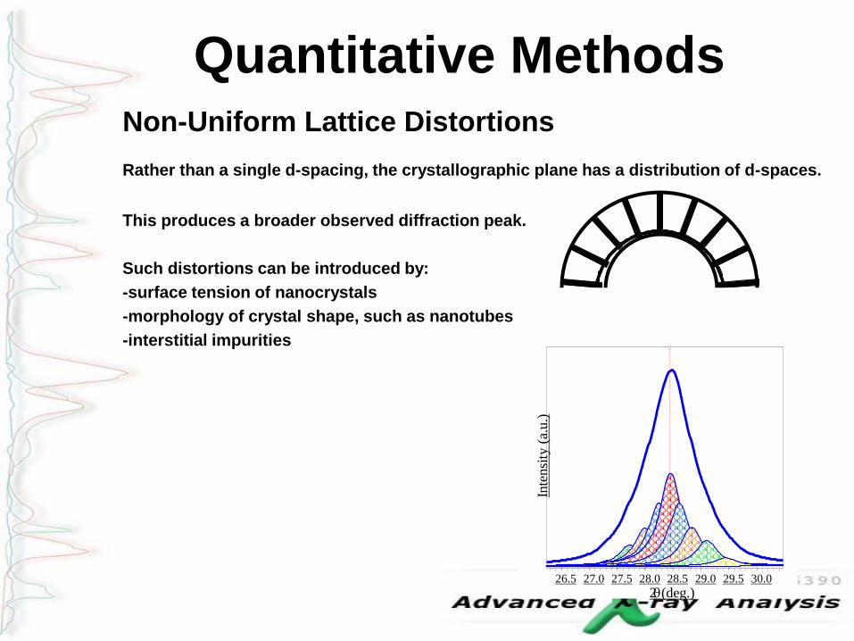
Quantitative MethodsNon-Uniform Lattice Distortions
Rather than a single d-spacing, the crystallographic plane has a distribution of d-spaces.
This produces a broader observed diffraction peak.
Such distortions can be introduced by:
-surface tension of nanocrystals
-morphology of crystal shape, such as nanotubes
-interstitial impurities
26.5 27.0 27.5 28.0 28.5 29.0 29.5 30.0
2q(deg.)
Inte
nsi
ty (
a.u.)

Quantitative MethodsAntiphase Domain Boundaries
Formed during the ordering of a material that goes through an order-disorder
transformation
The fundamental peaks are not affected
the superstructure peaks are broadened
The broadening of superstructure peaks varies with hkl
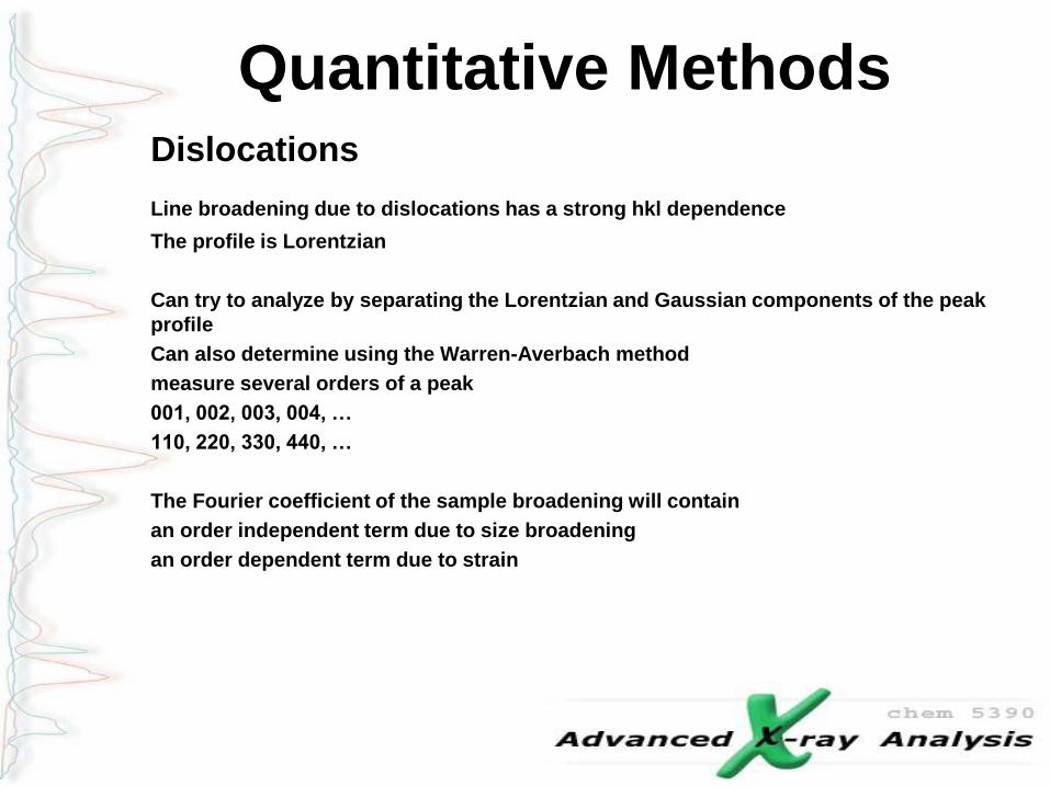
Quantitative MethodsDislocations
Line broadening due to dislocations has a strong hkl dependence
The profile is Lorentzian
Can try to analyze by separating the Lorentzian and Gaussian components of the peak
profile
Can also determine using the Warren-Averbach method
measure several orders of a peak
001, 002, 003, 004, …
110, 220, 330, 440, …
The Fourier coefficient of the sample broadening will contain
an order independent term due to size broadening
an order dependent term due to strain

Quantitative MethodsFaulting
Broadening due to deformation faulting and twin faulting will convolute with the particle
size Fourier coefficient
The particle size coefficient determined by Warren-Averbach analysis actually contains
contributions from the crystallite size and faulting
-the fault contribution is hkl dependent, while the size contribution should be hkl
independent (assuming isotropic crystallite shape)
-the faulting contribution varies as a function of hkl dependent on the crystal structure of
the material (fcc vs bcc vs hcp)
See Warren, 1969, for methods to separate the contributions from deformation and twin faulting

Quantitative MethodsSolid Solution Inhomogeneity
Variation in the composition of a solid solution can create a distribution of d-spacing for a
crystallographic plane
Similar to the d-spacing distribution created from microstrain due to non-uniform lattice
distortions
CeO2
19 nm
45 46 47 48 49 50 51 52
2q(deg.)
Inte
nsi
ty (
a.u
.)
ZrO2
46nmCexZr1-xO2
0<x<1

Quantitative MethodsTemperature Factor
The Debye-Waller temperature factor describes the oscillation of an atom around its
average position in the crystal structure
The thermal agitation results in intensity from the peak maxima being redistributed into the
peak tails
-it does not broaden the FWHM of the diffraction peak, but it does broaden the
integral breadth of the diffraction peak
The temperature factor increases with 2Theta
The temperature factor must be convoluted with the structure factor for each peak
-different atoms in the crystal may have different temperature factors
-each peak contains a different contribution from the atoms in the crystal
MfF exp
2
2 3/2
d
XM

Quantitative Methods
Stress Measurements
Broadening of a diffraction line due to stress can
be represented by:
be = 4etanq
where,
e – residual strain (also represented as h)
be – (radians) – broadening of observed
diffraction peak.

Quantitative Methods
Particle Size Measurements
Grain size in materials has an effect on the
material’s properties, i.e., strength, hardness,
etc…
When size of the individual crystals is less than
~ 0.1 mm (1000 Å) the term “particle size” or
“crystallite size” is used.

Quantitative Methods
Particle Size Measurements
Broadening of the diffraction lines due to small particle size can
be used to determine crystallite sizes of less than 1 mm.
Peak broadening is related to the mean crystallite size by the
Scherrer equation:
t = Kl/btcosqb
K – shape factor (usually 0.9)
bt – line broadening as FWHM for 2q due to small crystallites
(must be in radians)
t – crystallite size (diameter) (also represented as L or t)
bt = (b – binst) b – FWHM of observed diffraction line
binst – instrumental broadening
Quantitative Methods
Particle Size Measurements
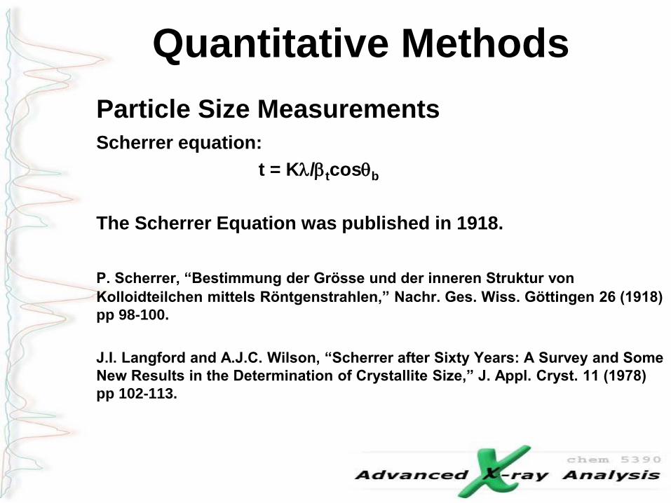
Scherrer equation:
t = Kl/btcosqb
The Scherrer Equation was published in 1918.
P. Scherrer, “Bestimmung der Grösse und der inneren Struktur von
Kolloidteilchen mittels Röntgenstrahlen,” Nachr. Ges. Wiss. Göttingen 26 (1918)
pp 98-100.
J.I. Langford and A.J.C. Wilson, “Scherrer after Sixty Years: A Survey and Some
New Results in the Determination of Crystallite Size,” J. Appl. Cryst. 11 (1978)
pp 102-113.

Quantitative Methods
Particle Size Measurements
Scherrer equation:
t = Kl/btcosqb
The constant of proportionality, K (the Scherrer constant) depends on the how
the width is determined, the shape of the crystal, and the size distribution
the most common values for K are:
0.94 for FWHM of spherical crystals with cubic symmetry
0.89 for integral breadth of spherical crystals w/ cubic symmetry
1, because 0.94 and 0.89 both round up to 1
K actually varies from 0.62 to 2.08
For an excellent discussion of K, refer to JI Langford and AJC Wilson, “Scherrer after sixty years: A
survey and some new results in the determination of crystallite size,” J. Appl. Cryst. 11 (1978) p102-113.

Quantitative Methods
Particle Size Measurements
Scherrer equation:
t = Kl/btcosqb
Though the shape of crystallites is usually irregular, can often approximate
shape as:
sphere, cube, tetrahedra, or octahedra
parallelepipeds such as needles or plates
prisms or cylinders
Most applications of Scherrer analysis assume spherical crystallite shapes
If we know the average crystallite shape from another analysis, we can select
the proper value for the Scherrer constant K

Quantitative Methods
Particle Size Measurements
In order to analyze crystallite size, we must deconvolute:
Instrumental Broadening from Sample Broadening
We must then separate the different contributions to sample
broadening:
Crystallite size and microstrain broadening of diffraction peaks

Quantitative Methods
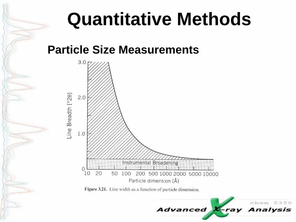
Particle Size Measurements
The peak width varies with 2q as cos q
The crystallite size broadening is most pronounced at large angles 2Theta
However, the instrumental profile width and microstrain broadening are also
largest at large angles 2theta
Peak intensity is usually weakest at larger angles 2theta
If using a single peak, often get better results from using diffraction peaks
between 30 and 50 deg 2theta
below 30deg 2theta, peak asymmetry compromises profile analysis
Quantitative Methods
Particle Size Measurements

Quantitative Methods
Instrumental FWHM Calibration Curve
• Standard should share characteristics with the nanocrystalline
specimen
– similar mass absorption coefficient
– similar atomic weight
– similar packing density
• The standard should not contribute to the diffraction peak profile
– macrocrystalline: crystallite size larger than 500 nm
– particle size less than 10 microns
– defect and strain free
• There are several calibration techniques
– Internal Standard
– External Standard of same composition
– External Standard of different composition

Quantitative Methods
Internal Standard Method for Calibration
Mix a standard in with your nanocrystalline specimen
a NIST certified standard is preferred
(use a standard with similar mass absorption coefficient)– NIST 640c Si
– NIST 660a LaB6
– NIST 674b CeO2
– NIST 675 Mica
Standard should have few, and preferably no, overlapping peaks with
the specimen– overlapping peaks will greatly compromise accuracy of analysis
Quantitative Methods
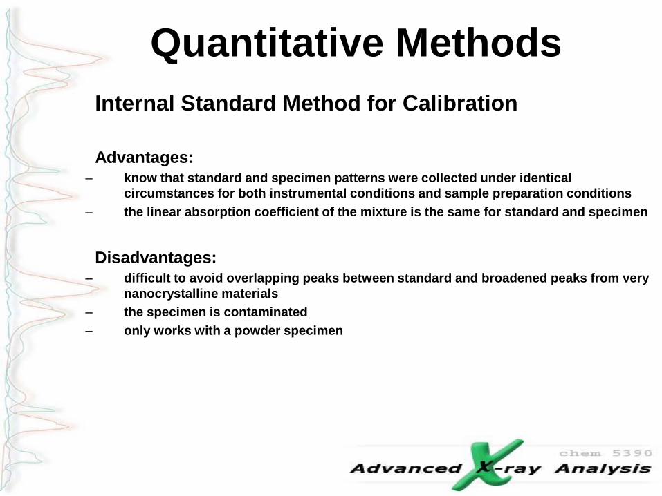
Internal Standard Method for Calibration
Advantages:– know that standard and specimen patterns were collected under identical
circumstances for both instrumental conditions and sample preparation conditions
– the linear absorption coefficient of the mixture is the same for standard and specimen
Disadvantages: – difficult to avoid overlapping peaks between standard and broadened peaks from very
nanocrystalline materials
– the specimen is contaminated
– only works with a powder specimen

Quantitative Methods
External Standard Method for Calibration
If internal calibration is not an option, then use external calibration
Run calibration standard separately from specimen, keeping as many
parameters identical as is possible
The best external standard is a macrocrystalline specimen of the same
phase as your nanocrystalline specimen
How can you be sure that macrocrystalline specimen does not
contribute to peak broadening?

Quantitative Methods
Qualifying your Macrocrystalline Standard
How can you be sure that macrocrystalline specimen does not
contribute to peak broadening?
select powder for your potential macrocrystalline standard
-if not already done, possibly anneal it to allow crystallites to grow and to
allow defects to heal
use internal calibration to validate that macrocrystalline specimen is
an appropriate standard
-mix macrocrystalline standard with appropriate NIST SRM
-compare FWHM curves for macrocrystalline specimen and NIST
standard
-if the macrocrystalline FWHM curve is similar to that from the NIST
standard, than the macrocrystalline specimen is suitable
-collect the XRD pattern from pure sample of you macrocrystalline
specimen
do not use the FHWM curve from the mixture with the NIST SRM

Quantitative Methods
Disadvantages/Advantages of External Calibration
with a Standard of the Same Composition
Advantages:
-will produce better calibration curve because mass absorption coefficient,
density, molecular weight are the same as your specimen of interest
-can duplicate a mixture in your nanocrystalline specimen
-might be able to make a macrocrystalline standard for thin film samples
Disadvantages:
-time consuming
-desire a different calibration standard for every different nanocrystalline phase
and mixture
-macrocrystalline standard may be hard/impossible to produce
-calibration curve will not compensate for discrepancies in instrumental
conditions or sample preparation conditions between the standard and the
specimen

Quantitative Methods
External Standard Method of Calibration using a
NIST standard
Use an external standard of a composition that is different than your
nanocrystalline specimen
This is actually the most common method used
Also the least accurate method
Use a certified NIST standard to produce instrumental FWHM
calibration curve

Quantitative Methods
Advantages and Disadvantages of using NIST
standard for External Calibration
Advantages:
-only need to build one calibration curve for each instrumental configuration
-know that the standard is high quality if from NIST
-neither standard nor specimen are contaminated
Disadvantages:
-The standard may behave significantly different in diffractometer than your
specimen
-different mass absorption coefficient
-different depth of penetration of X-rays
-NIST standards are expensive
-cannot duplicate exact conditions for thin films

Quantitative Methods

Quantitative Methods
0
50
100
150
200
(511)(422)
(331)(400)
(222)
(311)
(220)
(200)
(111)
Inte
nsit
y (
cp
s)
Inte
nsit
y (
cp
s)
a
Inte
nsit
y (
cp
s)
0
100
200
300
400
Ab
0
500
1000
1500
2000
2500
c
0
500
1000
1500
2000
2500
d
20 40 60 80 100
0
500
1000
1500
2000
2500
3000
3500
e
2q (degrees)
20 40 60 80 100
0
1000
2000
3000
4000 f
2q (degrees)
0 200 400 600 800 1000 1200
0
100
200
300
400
500
B
Gra
in S
ize (
nm
)
Sintering Temperature (oC)

Quantitative Methods
Broadening Effects
Since broadening by stress follows a tanq
function and broadening by crystallite size has a
1/cosq dependence, both effects can be
separated out during analysis.
Contributions can be separated if the peaks are
Lorenztian or Gaussian-shaped.

Quantitative Methods
Broadening Effects
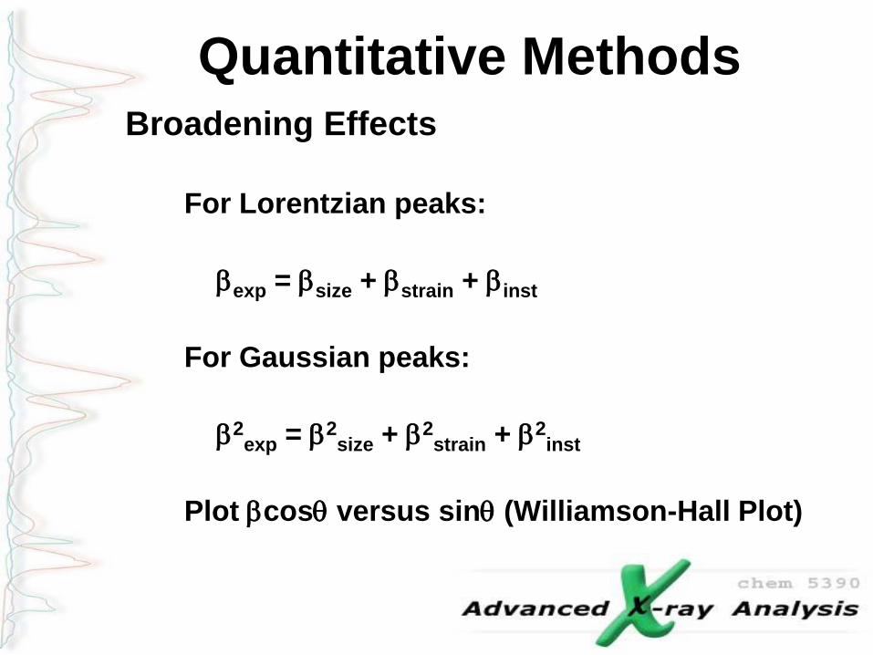
Quantitative MethodsBroadening Effects
For Lorentzian peaks:
bexp = bsize + bstrain + binst
For Gaussian peaks:
b2exp = b2
size + b2strain + b2
inst
Plot bcosq versus sinq (Williamson-Hall Plot)

Quantitative Methods

Quantitative Methods

Quantitative Methods
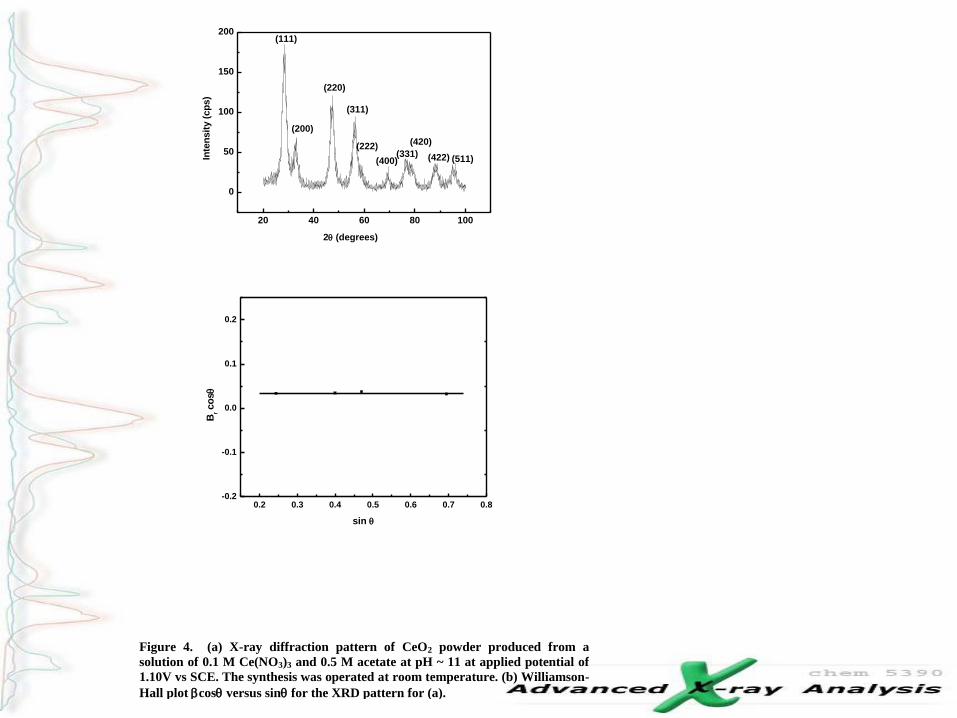
Broadening Effects – Ex: CeO2
Contributions of crystallite size and strain are given
by the following equation:
where
l is the wavelength of the x-rays,
q is the diffraction angle,
h is the strain,
L is the crystallite size,
k is a constant (0.94 for gaussian line profiles and small cubic
crystals of uniform size)
br is the corrected full width at half maximum of the peak
qhl
qb sincos L
kr

Quantitative Methods
Broadening Effects
br is the corrected full width at half maximum of the
peak given by,
where
bm is the experimental measured half width
bs is half width of a silicon powder standard with
peaks corresponding to the same 2q region.
222
smr bbb

Quantitative Methods
Broadening Effects – Williamson-Hall Plot
0.2 0.3 0.4 0.5 0.6 0.70.00
0.01
0.02
0.03
0.04
0.05
brc
osq
sinq
20 40 60 80 100
0
50
100
150
200
(511)
(420)(222)
(422)(331)(400)
(311)
(220)
(200)
(111)
Inte
nsit
y (
cp
s)
2q (degrees)
0.2 0.3 0.4 0.5 0.6 0.7 0.8-0.2
-0.1
0.0
0.1
0.2
Br c
osq
sin q
Figure 4. (a) X-ray diffraction pattern of CeO2 powder produced from a
solution of 0.1 M Ce(NO3)3 and 0.5 M acetate at pH ~ 11 at applied potential of
1.10V vs SCE. The synthesis was operated at room temperature. (b) Williamson-
Hall plot bcosq versus sinq for the XRD pattern for (a).


Reading Assignment:
Read Chapter 5, 6, and 7 from:
-Introduction to X-ray powder
Diffractometry by Jenkins and Synder
Read Chapter 13 from:
-Introduction to X-ray powder
Diffractometry by Jenkins and Synder
Read Chapter 13 and 14 from:
-Elements of X-ray Diffraction, 3rd edition, by Cullity and Stock
Lab 4: Precise Lattice Parameters
Tuesday, Oct. 30th 8:00 am
Group 1
Tuesday, Oct. 30th 8:30 am
Group 2
Thursday, Nov. 1st 8:00 am
Group 3
Thursday, Nov. 1st 8:30 am
Group 4
Take Home Test II – Pick up Nov 1st by 8:30 am.


![Rosetta Langmuir probe performance - DiVA portal680862/FULLTEXT01.pdf1.3.1 Debye shielding and Debye length Debye shielding [1] is an innate ability of the plasma to shield out local](https://img.pdfslide.us/doc/110x75/60ffba69c4d405429359b4af/rosetta-langmuir-probe-performance-diva-680862fulltext01pdf-131-debye-shielding.jpg)