Lecture 8 - IIR Filters (II) - Home - Walter Scott, Jr. … Lecture 8 Outline Introduction IIR Filter Design Overview Method: Impulse Invariance for IIR FIlters Approximation of Derivatives

Colorado State University Dept of Electrical and Computer Engineering ECE423 – 1 / 27

Lecture 8 - IIR Filters (II)

James Barnes ([email protected])

Spring 2009

Lecture 8 Outline


Introduction

Digital Filter Design by Analog → Digital Conversion

(Probably next lecture) ”All Digital” Design Algorithms

(Next lecture) Conversion of Filter Types by Frequency Transformation

Introduction

Lecture 8 Outline

Introduction IIR Filter DesignOverview

Method: ImpulseInvariance for IIR FIlters

Approximation ofDerivatives

Bilinear Transform

Matched Z-Transform


IIR Filter Design Overview


Methods which start from analog design

Impulse Invariance

Approximation of Derivatives

Bilinear Transform

Matched Z-transform

All are different methods of mapping the s-plane onto the z-plane

Methods which are ”all digital”

Least-squares

McClellan-Parks

Method: Impulse Invariance for IIR FIlters

Lecture 8 Outline

Introduction


Impulse Invariance

Impulse Invariance (2)



Impulse InvarianceProcedure Impulse InvarianceExample

Impulse InvarianceExample (2)


Bilinear Transform

Matched Z-Transform


Impulse Invariance


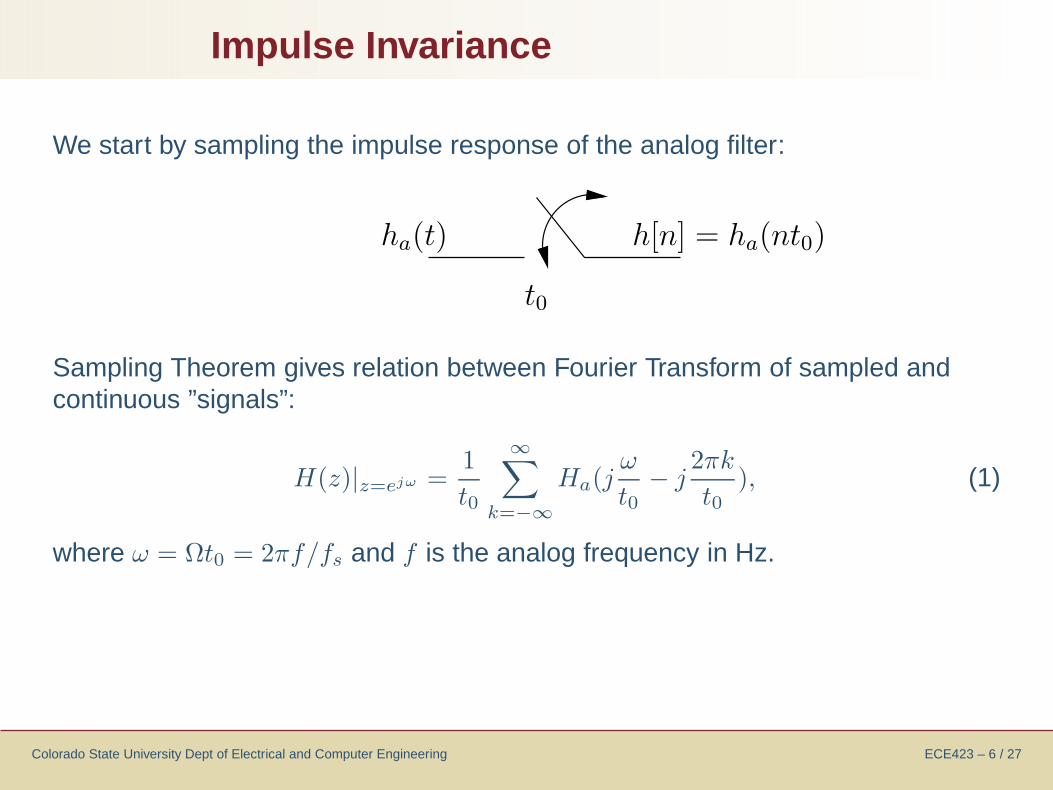
We start by sampling the impulse response of the analog filter:

ha(t) h[n] = h

a(nt0)

t0

Sampling Theorem gives relation between Fourier Transform of sampled andcontinuous ”signals”:

H(z)|z=ejω =1

t0

∞∑k=−∞

Ha(jω

t0− j

2πk

t0), (1)

where ω = Ωt0 = 2πf/fs and f is the analog frequency in Hz.



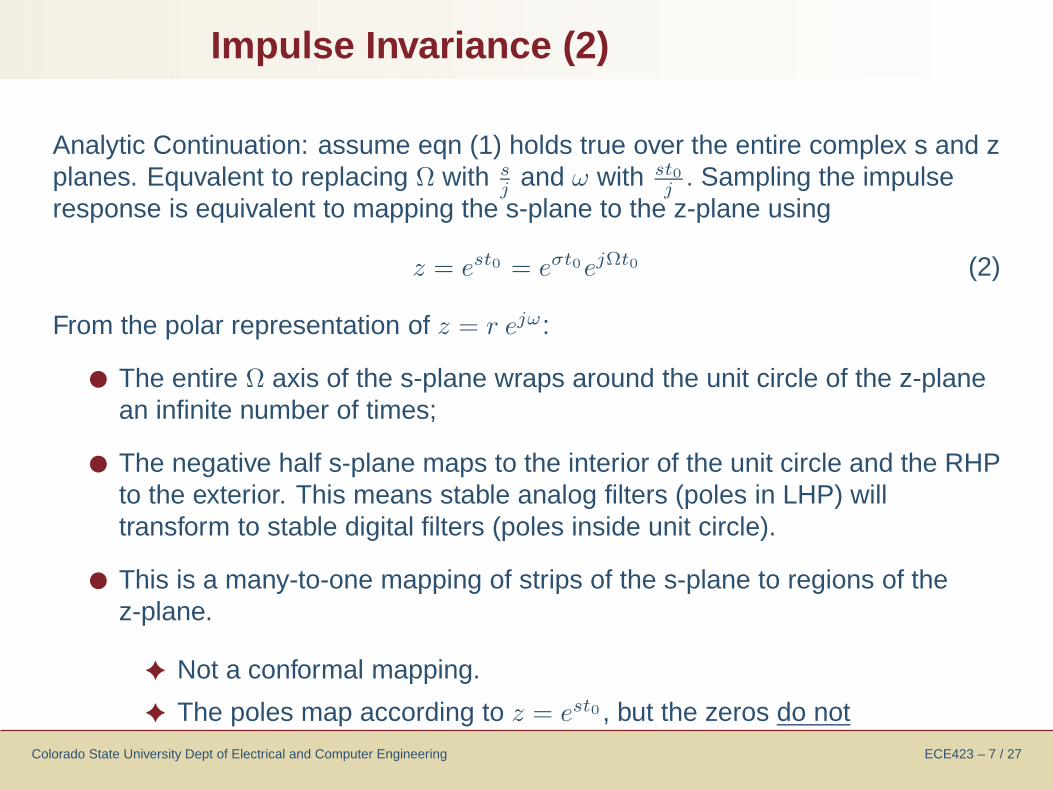
Analytic Continuation: assume eqn (1) holds true over the entire complex s and zplanes. Equvalent to replacing Ω with s

jand ω with st0

j. Sampling the impulse

response is equivalent to mapping the s-plane to the z-plane using

z = est0 = eσt0ejΩt0 (2)

From the polar representation of z = r ejω:

The entire Ω axis of the s-plane wraps around the unit circle of the z-planean infinite number of times;

The negative half s-plane maps to the interior of the unit circle and the RHPto the exterior. This means stable analog filters (poles in LHP) willtransform to stable digital filters (poles inside unit circle).

This is a many-to-one mapping of strips of the s-plane to regions of thez-plane.

Not a conformal mapping.

The poles map according to z = est0 , but the zeros do not



Mapping

jΩ

σ

. . .

. . .

πt0

s-plane

3 πt0

- πt0

1+j0

z-plane



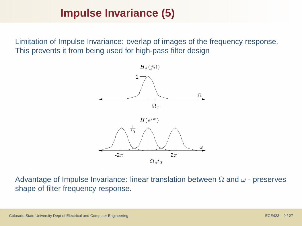
Limitation of Impulse Invariance: overlap of images of the frequency response.This prevents it from being used for high-pass filter design

2π

ω

H(ejω)

-2π

Ω

Ωct0

Ωc

Ha(jΩ)

1t0

1

Advantage of Impulse Invariance: linear translation between Ω and ω - preservesshape of filter frequency response.

Impulse Invariance Procedure


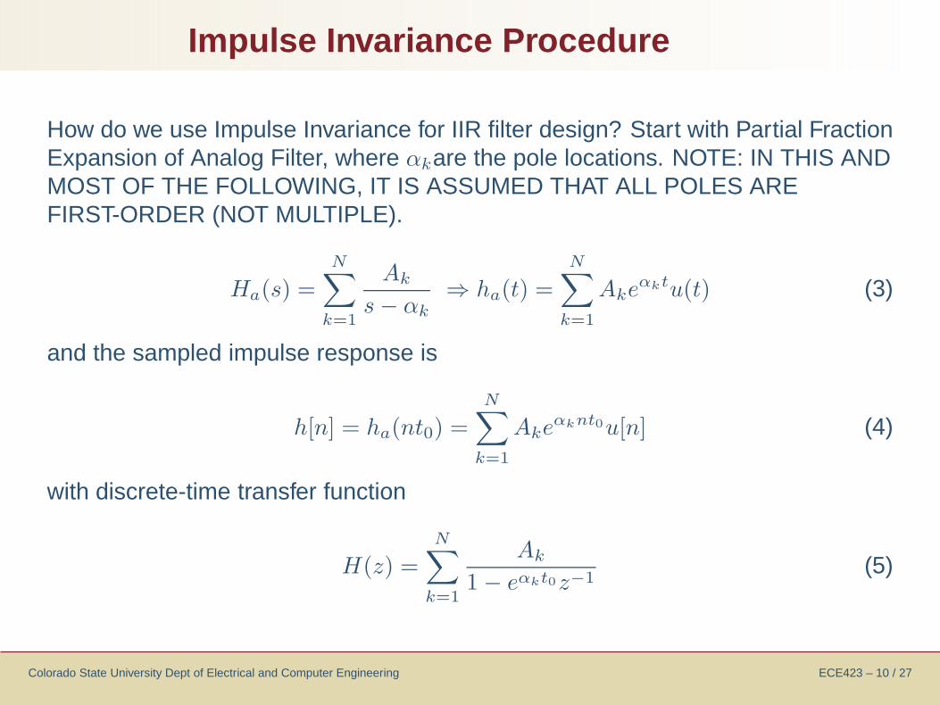
How do we use Impulse Invariance for IIR filter design? Start with Partial FractionExpansion of Analog Filter, where αkare the pole locations. NOTE: IN THIS ANDMOST OF THE FOLLOWING, IT IS ASSUMED THAT ALL POLES AREFIRST-ORDER (NOT MULTIPLE).

Ha(s) =

N∑k=1

Ak

s − αk

⇒ ha(t) =

N∑k=1

Akeαktu(t) (3)

and the sampled impulse response is

h[n] = ha(nt0) =N∑

k=1

Akeαknt0u[n] (4)

with discrete-time transfer function

H(z) =N∑

k=1

Ak

1 − eαkt0z−1(5)

Impulse Invariance Example


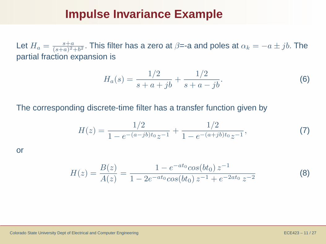
Let Ha = s+a(s+a)2+b2

. This filter has a zero at β=-a and poles at αk = −a ± jb. Thepartial fraction expansion is

Ha(s) =1/2

s + a + jb+

1/2

s + a − jb. (6)

The corresponding discrete-time filter has a transfer function given by

H(z) =1/2

1 − e−(a−jb)t0z−1+

1/2

1 − e−(a+jb)t0z−1, (7)

or

H(z) =B(z)

A(z)=

1 − e−at0cos(bt0) z−1

1 − 2e−at0cos(bt0) z−1 + e−2at0 z−2(8)

Impulse Invariance Example (2)


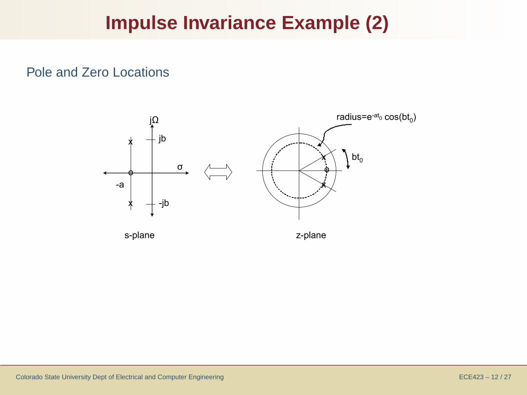
Pole and Zero Locations

Approximation of Derivatives

Lecture 8 Outline

Introduction


Approximation ofDerivatives Method:Approximation ofDerivatives Approximation ofDerivatives (2)

Approximation ofDerivatives (3)

Bilinear Transform

Matched Z-Transform


Method: Approximation of Derivatives


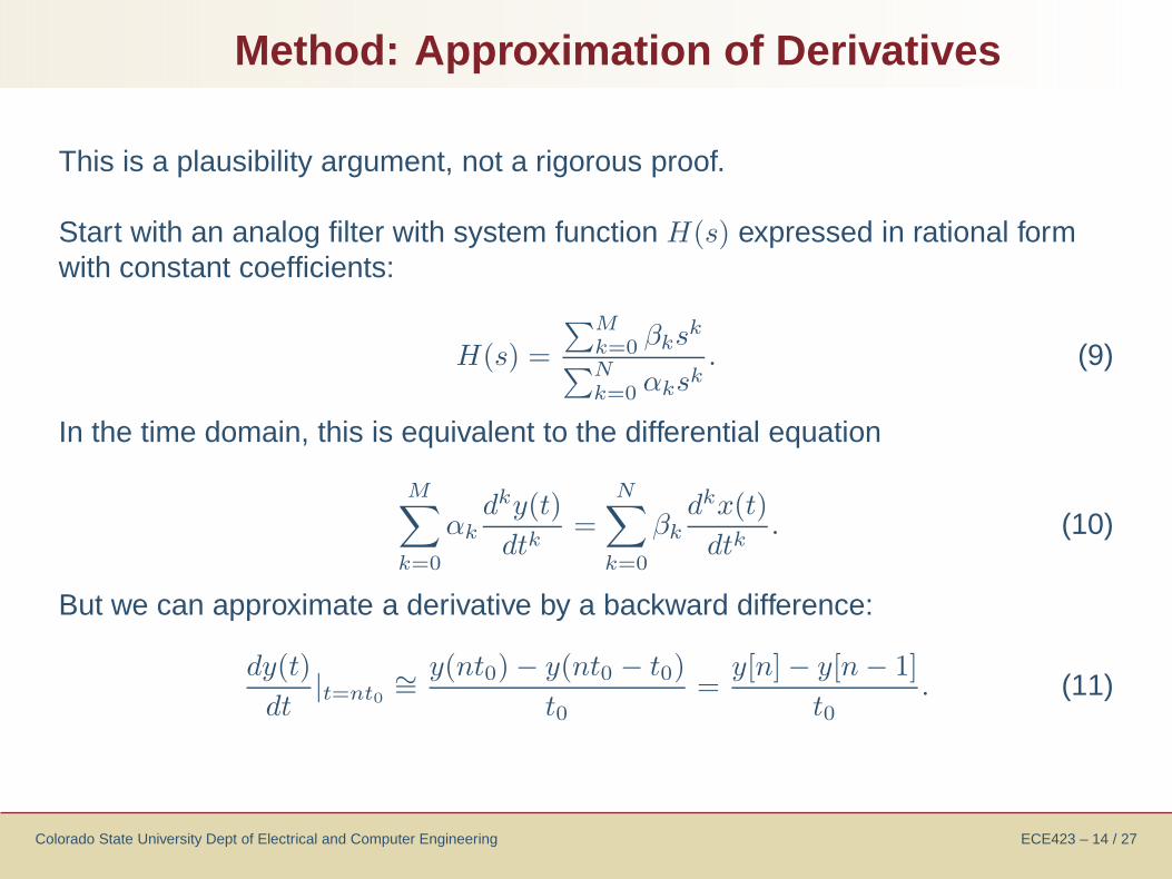
This is a plausibility argument, not a rigorous proof.

Start with an analog filter with system function H(s) expressed in rational formwith constant coefficients:

H(s) =

∑M

k=0 βksk

∑N

k=0 αksk. (9)

In the time domain, this is equivalent to the differential equation

M∑k=0

αk

dky(t)

dtk=

N∑k=0

βk

dkx(t)

dtk. (10)

But we can approximate a derivative by a backward difference:

dy(t)

dt|t=nt0

∼=y(nt0) − y(nt0 − t0)

t0=

y[n] − y[n − 1]

t0. (11)

Approximation of Derivatives (2)


The left hand and right hand sides of eqn(11) represent a continuous time anddiscrete time system which are supposed to be equivalent:

y[n]−y[n−1]t0

dydt

y(t)

y[n]H(z) =

1−z−1

t0

H(s) = s

For both systems to be equivalent, we must have the following mapping:

s =1 − z−1

t0. (12)

This relationship between s and z holds for all orders of the derivative, with sreplaced by skand the first order difference replaced by the k-th order difference.Hence it holds for the system described by eqn (10).

Approximation of Derivatives (3)


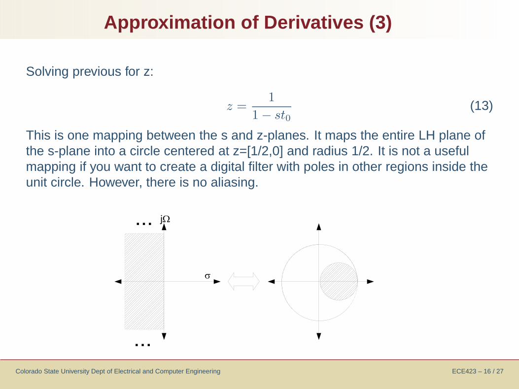
Solving previous for z:

z =1

1 − st0(13)

This is one mapping between the s and z-planes. It maps the entire LH plane ofthe s-plane into a circle centered at z=[1/2,0] and radius 1/2. It is not a usefulmapping if you want to create a digital filter with poles in other regions inside theunit circle. However, there is no aliasing.

Bilinear Transform

Lecture 8 Outline

Introduction



Bilinear Transform Method: BilinearTransform

Bilinear Transform (2)

Bilinear Transform -Pre-warping

Bilinear Transform -Pre-warping (2)

Design Example forSecond Order Section Second-order Section(2)

Second-order Section(3)

Matched Z-Transform


Method: Bilinear Transform


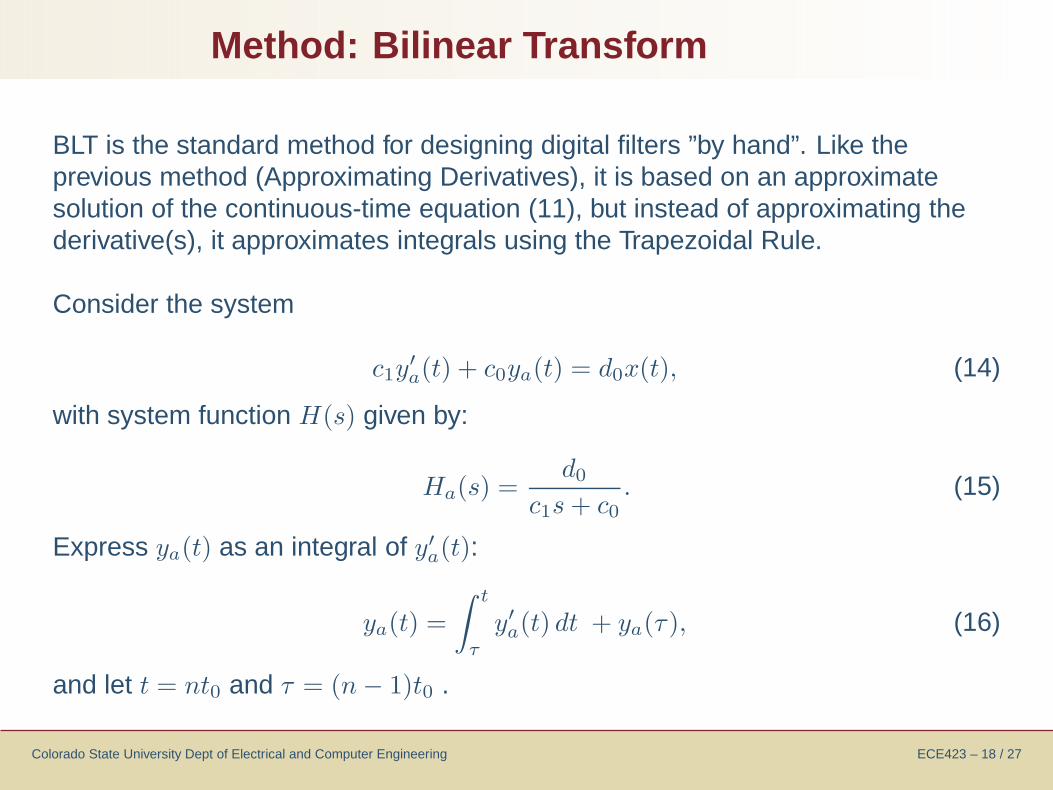
BLT is the standard method for designing digital filters ”by hand”. Like theprevious method (Approximating Derivatives), it is based on an approximatesolution of the continuous-time equation (11), but instead of approximating thederivative(s), it approximates integrals using the Trapezoidal Rule.

Consider the system

c1y′

a(t) + c0ya(t) = d0x(t), (14)

with system function H(s) given by:

Ha(s) =d0

c1s + c0. (15)

Express ya(t) as an integral of y′

a(t):

ya(t) =

∫ t

τ

y′

a(t) dt + ya(τ ), (16)

and let t = nt0 and τ = (n − 1)t0 .

Bilinear Transform (2)


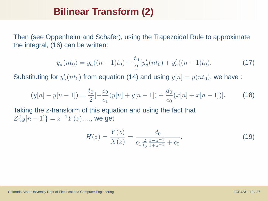
Then (see Oppenheim and Schafer), using the Trapezoidal Rule to approximatethe integral, (16) can be written:

ya(nt0) = ya((n − 1)t0) +t02

[y′

a(nt0) + y′

a((n − 1)t0). (17)

Substituting for y′

a(nt0) from equation (14) and using y[n] = y(nt0), we have :

(y[n] − y[n − 1]) =t02

[−c0

c1(y[n] + y[n − 1]) +

d0

c0(x[n] + x[n − 1])]. (18)

Taking the z-transform of this equation and using the fact thatZy[n − 1] = z−1Y (z), ..., we get

H(z) =Y (z)

X(z)=

d0

c12t0

1−z−1

1+z−1 + c0

. (19)

Bilinear Transform - Pre-warping


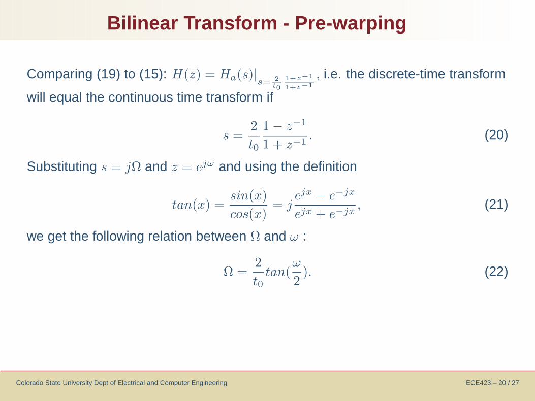
Comparing (19) to (15): H(z) = Ha(s)|s= 2

t0

1−z−1

1+z−1

, i.e. the discrete-time transform

will equal the continuous time transform if

s =2

t0

1 − z−1

1 + z−1. (20)

Substituting s = jΩ and z = ejω and using the definition

tan(x) =sin(x)

cos(x)= j

ejx − e−jx

ejx + e−jx, (21)

we get the following relation between Ω and ω :

Ω =2

t0tan(

ω

2). (22)

Bilinear Transform - Pre-warping (2)


The relation between Ω and ω and the mapping between s- and z-planes areshown below:

Note that the bilinear transform maps the entire left-hand s-plane to the interior ofthe unit circle of the z-plane, and that higher frequencies along the jΩ axis arecompressed compared with frequencies near 0.

Design Example for Second Order Section


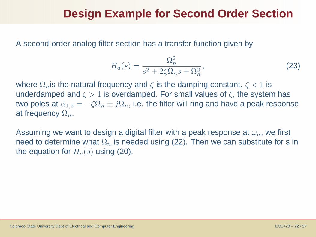
A second-order analog filter section has a transfer function given by

Ha(s) =Ω2

n

s2 + 2ζΩns + Ω2n

, (23)

where Ωnis the natural frequency and ζ is the damping constant. ζ < 1 isunderdamped and ζ > 1 is overdamped. For small values of ζ, the system hastwo poles at α1,2 = −ζΩn ± jΩn, i.e. the filter will ring and have a peak responseat frequency Ωn.

Assuming we want to design a digital filter with a peak response at ωn, we firstneed to determine what Ωn is needed using (22). Then we can substitute for s inthe equation for Ha(s) using (20).

Second-order Section (2)


One solution direct solution (messy, not as pretty as the next one):

H(z) = GB(z)

A(z)=

Γ2

Γ2 + 4Γζ + 4

1 + 2z−1 + z−2

1 + 2 (Γ2−4)Γ2+4Γζ+4z−1 + Γ2−4Γζ+4

Γ2+4Γζ+4z−2, (24)

Where Γ = Ωnt0 and G is the ”gain factor”. This solution doesn’t explicitly showthe pole locations (and probably could be simplified), but it is in the form suchthat a filter section could be implemented.

Second-order Section (3)


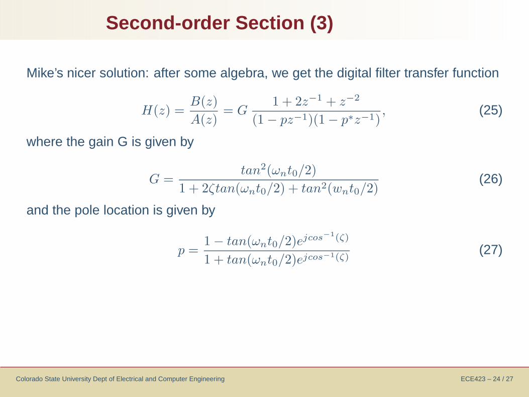
Mike’s nicer solution: after some algebra, we get the digital filter transfer function

H(z) =B(z)

A(z)= G

1 + 2z−1 + z−2

(1 − pz−1)(1 − p∗z−1), (25)

where the gain G is given by

G =tan2(ωnt0/2)

1 + 2ζtan(ωnt0/2) + tan2(wnt0/2)(26)

and the pole location is given by

p =1 − tan(ωnt0/2)ejcos−1(ζ)

1 + tan(ωnt0/2)ejcos−1(ζ)(27)

Matched Z-Transform

Lecture 8 Outline

Introduction



Bilinear Transform

Matched Z-Transform Method: MatchedZ-Transform Summary of Analog→ DigitalTransformation


Method: Matched Z-Transform


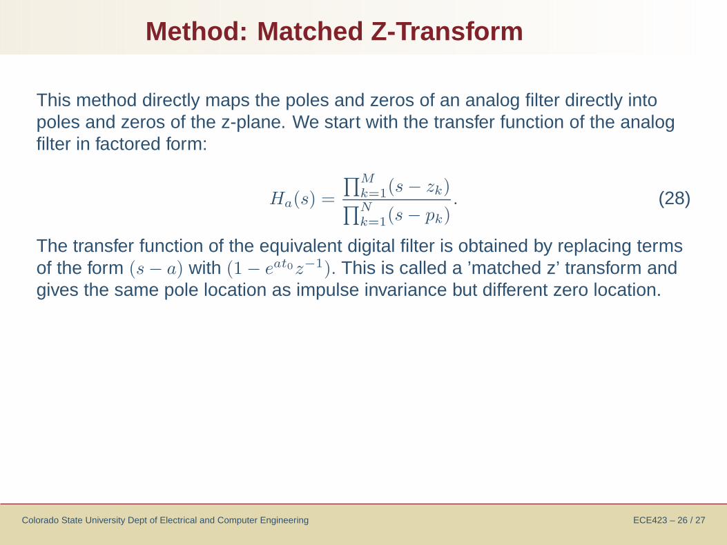
This method directly maps the poles and zeros of an analog filter directly intopoles and zeros of the z-plane. We start with the transfer function of the analogfilter in factored form:

Ha(s) =

∏M

k=1(s − zk)∏N

k=1(s − pk). (28)

The transfer function of the equivalent digital filter is obtained by replacing termsof the form (s − a) with (1 − eat0z−1). This is called a ’matched z’ transform andgives the same pole location as impulse invariance but different zero location.

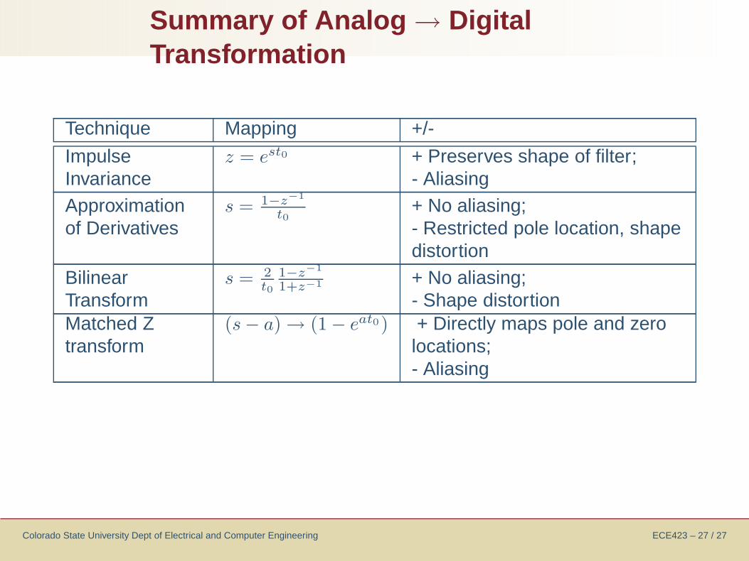
Summary of Analog → DigitalTransformation


Technique Mapping +/-

ImpulseInvariance

z = est0 + Preserves shape of filter;- Aliasing

Approximationof Derivatives

s = 1−z−1

t0+ No aliasing;- Restricted pole location, shapedistortion

BilinearTransform

s = 2t0

1−z−1

1+z−1 + No aliasing;- Shape distortion

Matched Ztransform

(s − a) → (1 − eat0) + Directly maps pole and zerolocations;- Aliasing

Documents

Lecture 8 - IIR Filters (II) - Home - Walter Scott, Jr. … Lecture 8 Outline Introduction IIR Filter Design Overview Method: Impulse Invariance for IIR FIlters Approximation of Derivatives