Embed Size (px)
Citation preview
Structural Mechanics 2.080 Lecture 8 Semester Yr
Lecture 8: Energy Methods in Elasticity
The energy methods provide a powerful tool for deriving exact and approximate solutions
to many structural problems.
8.1 The Concept of Potential Energy
From high school physics you must recall two equations
E =1
2Mv2 kinematic energy (8.1a)
W = mgH potential energy (8.1b)
where H is the hight of a mass m from a certain reference level Ho, and g stands for the
earth acceleration. The reference level could be the center of the earth, the sea level or any
surface from which H is measured.
H
m
F = mg
x
Ho
Ho
H
F
x
Figure 8.1: Gravitational potential energy.
We seldom measure H from the center of earth. Therefore what we can easily measure
is the change of the potential energy
∆W = (mg)(H −Ho) (8.2)
The energy is always positive. It can e zero but it cannot be negative. The gravity force
F = mg is directed towards the center of earth. Therefore there is a need for the negative
sign in Eq. (8.2)). In the coordinate system of Fig. (8.1), the gravity force is negative
(opposite to the sense of coordinate x). The force F is acting in the sense of x but the
difference H −Ho is negative.
Extending the concept of the potential energy to the beam, the force is F = q dx and
the w = H −Ho is the beam deflection.
W ≡ +
∫ l
0qw dx (8.3)
An analogous expression for plates is
W ≡ +
∫Spw ds (8.4)
8-1

Structural Mechanics 2.080 Lecture 8 Semester Yr
q
z dx
w
x
z
w
H Ho
q(x)
Figure 8.2: Potential energy of a beam element and the entire beam.
In the above definition W is negative.
The concept of the energy stored elastically U has been introduced earlier. For a 3-D
body
U =
∫V
1
2σijεij dv (8.5)
and for a beam
U =
∫ l
0
1
2MK dx+
∫ l
0
1
2Nε◦ dx (8.6)
For plates, the bending and membrane energies are given by Eqs. (4.73), (4.74) and (4.86),
(4.87).
The total potential energy Π is a new concept, and it is defined as the sum of the drain
energy and potential energy
Π = U + (−W ) = U −W (8.7)
Consider for a while that the material is rigid, for which U ≡ 0. Imagine a rigid ball
being displaced by an infinitesimal amount on a flat (θ = 0) and inclined (θ 6= 0) surface,
Fig. (8.3).
x
x θ δu
δu
H δH
Figure 8.3: Test if an infinitesimal displacement δu causes the potential energy to change.
We have H = u sin θ and δH = δu sin θ. The total potential energy and its change is
Π = −W = −Fu sin θ (8.8a)
δΠ = −δW = −(F sin θ)δu (8.8b)
On the flat surface, θ = 0 and δΠ = 0, and the ball is in static (neutral) equilibrium. If
θ > 0, δΠ 6= 0 and the ball is not in static equilibrium. Note that if the d’Alambert inertia
8-2

Structural Mechanics 2.080 Lecture 8 Semester Yr
force in the direction of motion is added, the ball will still be in dynamic equilibrium. In
this lecture, only static equilibrium is considered. We can now extend the above test for
equilibrium and introduce the following principle:
The system is said to be in equilibrium, if an infinitesimal change of the argument a of
the total potential energy Π = Π(a) does not change the total potential energy
δΠ(a) =∂Π
∂aδa = 0 (8.9)
Because δa 6= 0 (δa = 0 is a trivial case in which no test for equilibrium is performed), the
necessary and sufficient condition for stability is
∂Π
∂a= 0 (8.10)
In case when the functional Π is a function of many (say N) variables Π = Π(ai), the
increment
δΠ =∂Π
∂aiδai, i = 1, ..., N (8.11)
The system is in equilibrium if the derivative of Π with respect to each variable at a time
vanishes∂Π(ai)
∂ai= 0, i = 1, ..., N (8.12)
The meaning of the argument(s) ai, or independent variables will be explained next.
8.2 Equivalence of the Minimum Potential Energy and Prin-
ciple of Virtual Work
The concept of virtual displacement δui is the backbone of the energy methods in mechanics.
The virtual displacement is a small hypothetical displacement which satisfy the kinematic
boundary condition. The virtual strains δεij are obtained from the virtual displacement by
δεij =1
2(δui,j + δuj,i) (8.13)
The increment of stress δσij corresponding to the increment of strain is obtained from the
elasticity law
σij = Cijklεkl (8.14a)
δσij = Cijklδεkl (8.14b)
Therefore, by eliminating Cijklσijδεij = εijδσij (8.15)
The total strain energy of the elastic system Π is the sum of the elastic strain energy stored
and the work of external forces
Π =
∫V
1
2σijεij dv −
∫STiui ds (8.16)
8-3
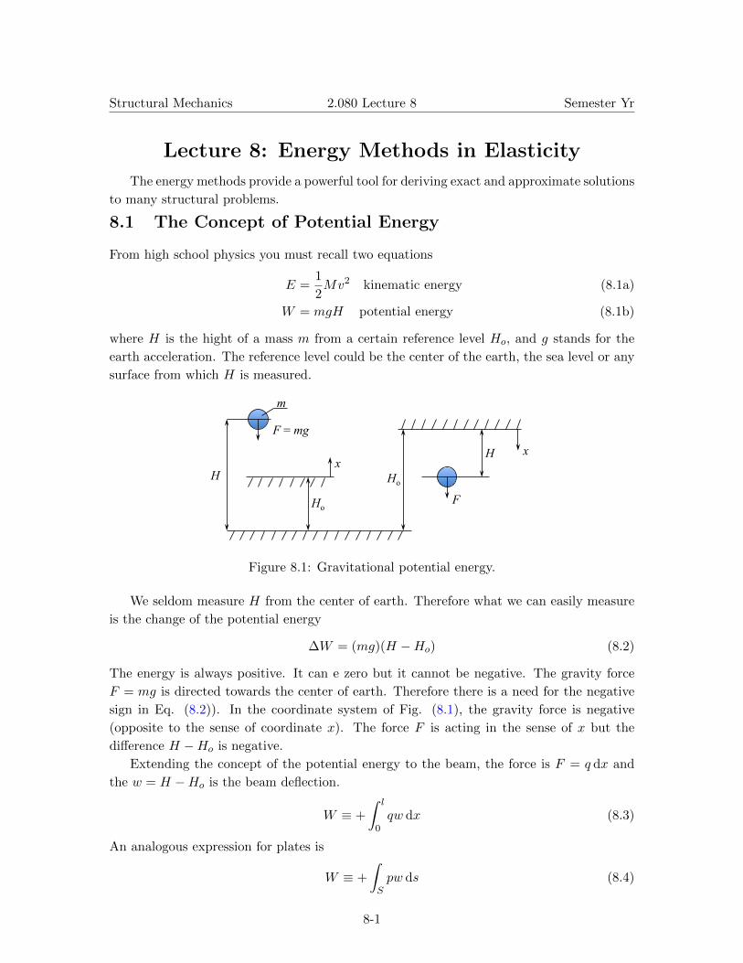
Structural Mechanics 2.080 Lecture 8 Semester Yr
σ
ε
δσ
δε ε
σ
Figure 8.4: Equivalence of the strain energy and complementary strain energy.
In the above equation the surface traction are given and considered to be constant.
The stresses σij are not considered to be constant because they are related to the variable
strains. For equilibrium the potential energy must be stationary, δΠ = 0 or
δ
∫V
1
2σijεij dv − δ
∫STiui ds
=1
2
∫Vδ(σijεij) dv −
∫STiδui ds
=1
2
∫V
(δσijεij + σijδεij) dv −∫STiδui ds = 0
(8.17)
The two terms in the integrand of the volume integral are equal in view of Eq. (8.15).
Therefore, Eq. (8.17) can be written in the equivalent form∫Vσijδεij dv =
∫STiδui ds (8.18)
which is precisely the principle of virtual work. The above proof goes also in the opposite
direction. Assuming the principle of virtual work one can show that the stationarity of the
total potential energy holds.
8.3 Two Formulations for Beams
In the bending theory of beams, the total potential energy is
Π =
∫ l
0
1
2Mκ dx−
∫ l
0q(x)w dx (8.19)
Using the moment curvature relation M = EIκ, either M or κ can be eliminated from Eq.
(8.18), leading to
U =
∫ l
0
1
2Mκ dx =
∫ l
0
EI
2κ2 dx displacement formulation∫ l
0
1
2EIM2 dx stress formulation
(8.20)
8-4

Structural Mechanics 2.080 Lecture 8 Semester Yr
In statically determined problems the bending moments can be expressed in terms of
the prescribed line load or point load. In the latter case the M = M(P ) and the total
potential energy takes the form
Π = U(P )− Pw (8.21)
The above representation will lead to the Castigliano theorem which will be covered later
in this lecture.
The more general displacement formulation will be covered next. The curvature is
proportional to the second derivative of the displacement. The expression of the total
potential energy becomes
Π =
∫ l
0
EI
2(w′′)2 dx−
∫ l
0q(x)w dx (8.22)
The problem is reduced to express the displacement field in terms of a finite number of free
parameters w(x, ai) and then use the stationary condition, Eq. (8.12) to determine these
unknown parameters. This could be done in three different ways:
(i) Polinomial representation or Taylor series expansion
(ii) Fourier series expansion
(iii) FInite element or finite difference method
Each of the above procedure will be explained separately.
8.4 Fourier Series Expansion and the Ritz Method
Consider a symetrically loaded simply supported plate by the point force at the center. The
total potential energy of the system is
Π =
∫ l
0
EI
2(w′′)2 dx− Pw (8.23)
The objective is to find the amplitude and shape of the deflection function that is in equi-
librium with the prescribed load P . In other words we will be looking the deflection and
shape that will make the total potential energy stationary.
Assume the solution as a Fourier expansion function
w(x) =N∑n=1
anφn(x) (8.24)
where φn(x) is a complete system of coordinate function satisfying kinematic boundary
conditions. In the rectangular coordinate system this system consists of hormonic functions,
8-5

Structural Mechanics 2.080 Lecture 8 Semester Yr
in the polar coordinate system these are Bessel function, and in the spherical coordinate
system this role is taken by the Legender functions. In our case
φn(x) = sinnπx
l(8.25)
The kinematic boundary conditions φn(x = 0) = φn(x = l) are identically satisfied. Further-
more, because of the symmetry of the problem, only the symmetric function will contribute
to the solution.
n = 2
n = 4
n = 1
n = 3
Figure 8.5: Asymmetric modes do not satisfy boundary condition w′(x =l
2) = 0 at the
center of the beam.
The solution is then represented as
w(x) = a1 sinπx
l+ a3 sin
3πx
l+ · · · (8.26)
Consider first one-term approximation
w(x) = a1 sinπx
l(8.27a)
w′(x) = a1
(πl
)cos
πx
l(8.27b)
w′′(x) = −a1(πl
)2sin
πx
l(8.27c)
The expression for the total potential energy is
Π =1
2EI(πl
)4a21
∫ l
0sin
πx
ldx− Pa1 (8.28)
where the integral is simply l/2. Eq. (8.26) reduces then to
Π =1
4EI
π4
l3a21 − Pa1 (8.29)
For equilibriumdΠ
da1= 0, which yields
1
2EI
π4
l3a1 − P = 0 (8.30)
8-6

Structural Mechanics 2.080 Lecture 8 Semester Yr
The load-displacement relation is finally given by
(a1)opt =Pl3
π4
2 EI=
Pl3
48.7EI(8.31)
The numerical coefficient in the exact solution of this problem is 48. The error of the
approximate solution is 1.4%. Such a good accuracy of just one-term approximation can be
explained by making the Taylor series expansion of the sign function
sinπx
l=πx
l− 1
6
(πxl
)3+ · · · (8.32)
The two term expansion has a linear and cubic terms in x, the same as the exact solution.
Let’s examine next the stationary property of the functional Π. Defining the normalized
total potential energy as Π̄ =Π
Pwo, one gets
Π̄ =1
2
a1wo
(a1wo− 2
)(8.33)
where a1 is the amplitude of the trial function Eq. (8.25) and wo is the exact amplitude.
The plot of the function Π̄(a1) is shown in Fig. (8.6).
⇧̄
a1
wo2.0 1.0 0
�1
2 Stationary point
Figure 8.6: By varying the amplitude arounda1wo
= 1, Π̄ does not change.
The function Π̄(a1) is a parabola with a stationary point at a1 = wo. The stationary
point is at the same time the minimum. The negative value of the minimum (actual) value
of the total potential energy comes from the choice of the reference level of the potential
energy. In mechanics, the reference level is the position of the undeformed axis of the beam.
Upon loading, the beam is loosing the potential energy and the second term in Eq. (8.21)
is negative and larger than the first term of the stored elastic energy.
Even though the accuracy of one term approximation in the Fourier series expansion, Eq.
(8.22) gave a very good approximation (1.4% error), the solution can be further improved
by considering the next term in the expansion, according to Eq. (8.24). In this case the
8-7

Structural Mechanics 2.080 Lecture 8 Semester Yr
total potential energy is the function of two unknown amplitudes, Π = Π(a1, a3) and the
solution is obtained from two algebraic equations
∂Π
∂a1= 0,
∂Π
∂a3= 0 (8.34)
8.5 Solution by Taylor expansion
Consider the same sample problem of the cantilever beam under the tip point force. Assume
the solution as a power series
w(x) =N∑n=1
anxn (8.35)
For illustration, truncate the series by taking the four first terms
w(x) = a0 + a1x+ a2x2 + a3x
3 (8.36)
The kinematic boundary conditions are
w(x = 0) = 0; w′(x = 0) = 0 (8.37)
It is easy to see that displacement boundary conditions are met if ao = a1 = 0. The
displacements, slopes and curvature become
w(x) = a2x2 + a3x
3 (8.38a)
w′(x) = 2a2x+ 3a3x2 (8.38b)
w′′(x) = 2a2 + 6a3x (8.38c)
The tip displacement is
w(x = l) = wo = a2l2 + a3l
3 (8.39)
The expression for the total potential energy is
Π =EI
2
∫ l
0(2a+ 6a3x)2 dx− P (a2l
2 + a3l3) (8.40)
or after integration
Π =EI
2(4a22l + 12a2a3l
2 + 12a23l3)− P (a2l
2 + a3l3) (8.41)
The stationary of Π(a2, a3) implies that
∂Π
∂a2= 0,
∂Π
∂a3= 0 (8.42)
which leads to two linear algebraic equations for a2, a3
4a2 + 6a3l =Pl
EI(8.43a)
6a2 + 12a3l =Pl
EI(8.43b)
8-8

Structural Mechanics 2.080 Lecture 8 Semester Yr
where solution is
a2 =Pl
2EI, a3 = − P
6EI(8.44)
The deflection of the beam is then
w(x) =P
EI
(lx2
2− x3
6
)(8.45)
The tip deflection is obtained
wo = w(x = l) =Pl3
3EI(8.46)
This is the exact solution of the problem. The exact solution was obtained in this case
because the first four terms of the Taylor expansion contained the actual deflected shape.
Note that the exact solution was obtained by the Ritz method without imposing the static
boundary conditions at the tip V = −P and M = 0. The graphical interpretation of the
stationary condition with two degrees of freedom is obtained by plotting Eq. (8.35) in the
space (Π, a2, a3), Fig. (8.7).
Π
a2
a3 0
Figure 8.7: The potential energy as a paraboloid.
8.6 Castigliano Theorem
This theorem applies to statically determined structures and system subjected to concen-
trated forces or moments. The distribution of bending moments can be uniquely determined
from global equilibrium as function of the forces, U = U(P ). The total potential energy is
Π = U(P )− Pwo (8.47)
8-9

Structural Mechanics 2.080 Lecture 8 Semester Yr
For a given deflection amplitude wo, the magnitude of the load adjust itself so as to
make the total potential energy stationary. Mathematically
δ[Π(P )] = δ[U(P )− Pwo] =dU
dPδP − woδP =
[dU(P )
dP− wo
]δP = 0 (8.48)
We have proved that the displacement under the force in the direction of the force is
equal to the derivative of the elastic energy stored with respect to the force.
In order to interpret the stationary property of Π, consider a cantilever beam with the
force P at its tip. The bending moment distribution is M(x) = P (l − x). Let’s choose the
force formulation of the total potential energy, Eq. (??). The total potential energy is
Π =P 2
2EI
∫ l
0(l − x)2dx− Pwo (8.49)
After integration
Π(P ) = P
(Pl3
6EI− wo
)(8.50)
The plot of this function is shown in Fig (8.8).
0
Π(P)
P 6EIwo
l3
3EIwo
l3
Figure 8.8: Parabolic variation of the total potential energy with the force P for a given
central deflection.
The parabola has two roots at P1 = 0 and at P2 =6EIwol3
. The stationary point is at
P =3EIwol3
(8.51)
which is the exact solution of the problem.
As an illustration, consider two simple structural systems. The first system of two beams
is shown in Fig. (8.9).
This problem was solved earlier using displacements and slope continuity. A much simple
solution follows. The bending moment distributions are
Beam (A) M(x) = −Px 0 < x < l
Beam (B) M(x) = 12Px 0 < x < l
Beam (C) M(x) = −12Px 0 < x < l
(8.52)
8-10

Structural Mechanics 2.080 Lecture 8 Semester Yr
B
C A
A C
B l
l
l P
x
x
x
P
Figure 8.9: Statically determined system and bending moment distribution.
The bending strain energy is
U(P ) =
∫ l
0
1
2EI
[P 2 +
(P
2
)2
+
(P
2
)2]x2 dx =
3
2P 2 l
3
3=
1
2P 2l3 (8.53)
From the relative contributions of the three beams in Eq. (8.44), it is seen that the
horizontal cantilever contributes twice to the tip deflection compared to the vertical beam.
l
l
B
A
P wB wA
wo
Figure 8.10: two welded beams forming an elbow.
The second system consists of an elbow. From Fig. (8.10), the bending moment distri-
bution is
Beam (A) M(x) = Px
Beam (B) M(x) = Pl(8.54)
The elastic bending energy of the system is
U(P ) =1
2EI
∫ l
0(Px)2 dx+
1
2EI
∫ l
0(Pl)2 dx =
P 2
2EI
4l3
3(8.55)
8-11

Structural Mechanics 2.080 Lecture 8 Semester Yr
The total deflection in the direction of the force is
wo =dU
dP=
4
3
Pl3
EI(8.56)
Proof of the Castigliano Theorem for a system of point loads, Pi
The corresponding displacements are denoted by wi, see Fig. (8.11).
P1 P2
w1 w2
Figure 8.11: An elastic body (structure) loaded by a system of concentrated forces.
The work of external forces is
W =∑i
Piwi = Piwi (8.57)
It is assumed that the energy stored can be expressed in terms of all the point forces,
U = U(Pi). Let’s keep all point forces at fixed values and vary only one, say Pk. For
equilibrium, the total potential energy of the system should be stationary with respect to
this change. Thus,
δΠ = δ(U −W ) =dU
dPkδPk − wkδPk
=
(dU
dPk− wk
)δPk = 0
(8.58)
The extended Castigliano theorem is
wk =∂U(Pi)
∂Pk(8.59)
For example, if there are two point loads applied,
w2 =∂U(P1, P2)
∂P2(8.60)
Usually the Castigliano theorem gives only deflection at a given point but not the
deflected shape. The extended theorem ca be used to predict the deflected shape.
8-12

Structural Mechanics 2.080 Lecture 8 Semester Yr
P P1
η
l x
w1 w
A B
Figure 8.12: Cantilever beam loaded b two point forces.
Illustration
Consider a cantilever beam loaded by two point forces. One force P is applied at the tip
and the other force P1 acts at a distance η from the support.
The bending moment distribution is
MA(x) = P (l − x) + P1(η − x) for 0 < x < η
MB(x) = P (l − x) for η < x < l(8.61)
The bending strain energy is
U(P, P1) =1
2EI
∫ η
0M2A dx+
1
2EI
∫ l
ηM2B dx (8.62)
According to Eq. (8.49), the deflection under the point load P1 is
w1 =∂U(P, P1)
∂P1=
1
EI
∫ η
0MA
∂MA
∂P1dx+
1
EI
∫ l
ηMB
∂MB
∂P1dx (8.63)
The derivatives of the bending moments are
∂MA
∂P1= η − x (8.64a)
∂MB
∂P1= 0 (8.64b)
Substituting Eqs. (8.51) and (??) into (??), one gets
w1 =1
EI
∫ η
0[P (l − x) + P1(η − x)](η − x) dx (8.65)
This equation is valid for any combination of P and P1. We can therefore assume that
P1 is a “dummy” force and can be set equal to zero. Then, Eq. (??) reduces to
w1 =1
EI
∫ η
0P (l − x)(η − x) dx (8.66)
8-13

Structural Mechanics 2.080 Lecture 8 Semester Yr
which gives, after integration,
w1(η) =Pl3
3EI
[3
2
(ηl
)2− 1
2
(ηl
)3](8.67)
In the above solution η is an arbitrary position along the beam and w1(η) is the correspond-
ing deflection. By changing the variables
η → x
w1(η) = w(x)(8.68)
we can recover the exact deflected shape of the cantilever beam
w(x) =Pl3
3EI
[3
2
(xl
)2− 1
2
(xl
)3](8.69)
The above example illustrated a great flexibility of the Castigliano method in solving stat-
ically determined problems.
8-14

MIT OpenCourseWarehttp://ocw.mit.edu
2.080J / 1.573J Structural MechanicsFall 2013
For information about citing these materials or our Terms of Use, visit: http://ocw.mit.edu/terms.