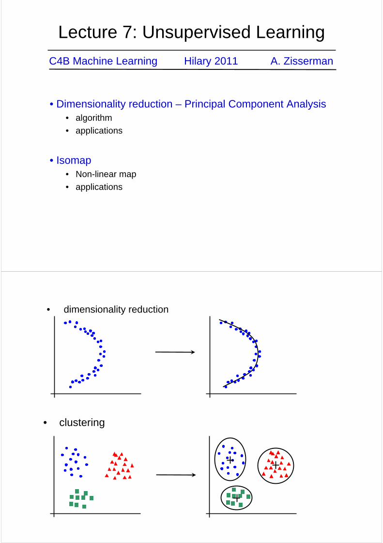
Lecture 7: Unsupervised Learning

C4B Machine Learning Hilary 2011 A. Zisserman

• Dimensionality reduction – Principal Component Analysis• algorithm

• applications

• Isomap• Non-linear map

• applications

• clustering

• dimensionality reduction

Dimensionality Reduction

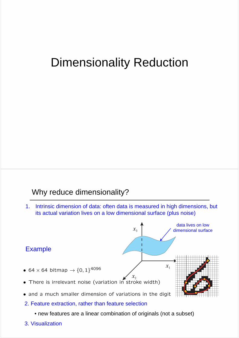
Why reduce dimensionality?

1. Intrinsic dimension of data: often data is measured in high dimensions, but its actual variation lives on a low dimensional surface (plus noise)

Example

x1

x1

x3

x3

x2

x2

data lives on low dimensional surface

• 64× 64 bitmap → {0,1}4096

• There is irrelevant noise (variation in stroke width)

• and a much smaller dimension of variations in the digit2. Feature extraction, rather than feature selection

• new features are a linear combination of originals (not a subset)

3. Visualization

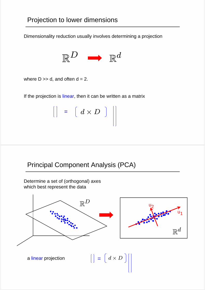
Projection to lower dimensions

Dimensionality reduction usually involves determining a projection

where D >> d, and often d = 2.

If the projection is linear, then it can be written as a matrix

RD Rd

d×D=

Principal Component Analysis (PCA)

Determine a set of (orthogonal) axes which best represent the data

u1

u2RD

Rd

a linear projection d×D=

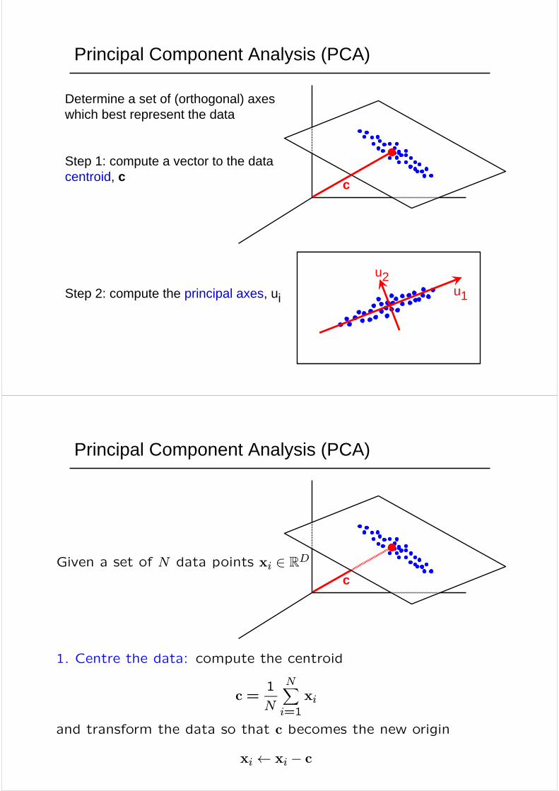
Principal Component Analysis (PCA)

Determine a set of (orthogonal) axes which best represent the data

Step 1: compute a vector to the data centroid, c

Step 2: compute the principal axes, ui

c

u1

u2

Principal Component Analysis (PCA)

cGiven a set of N data points xi ∈ RD

1. Centre the data: compute the centroid

c =1

N

NXi=1

xi

and transform the data so that c becomes the new origin

xi ← xi − c

Principal Component Analysis (PCA)

u

u

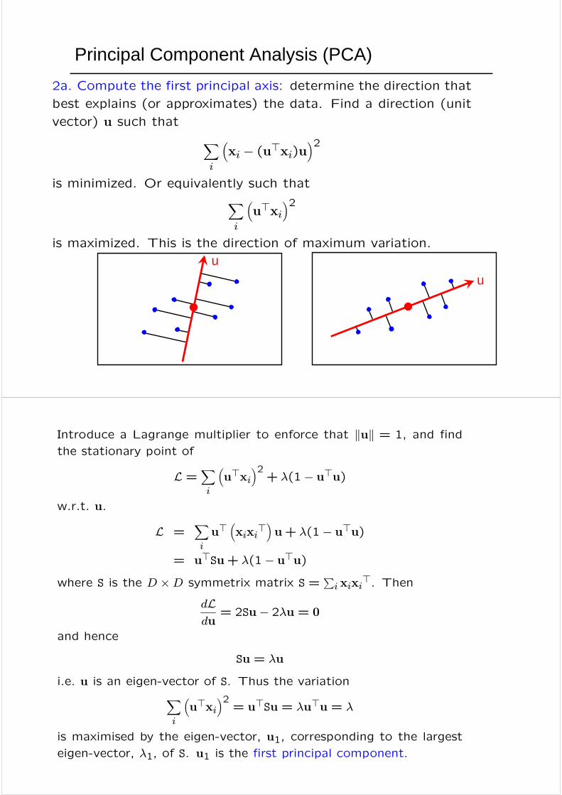
2a. Compute the first principal axis: determine the direction that

best explains (or approximates) the data. Find a direction (unit

vector) u such that Xi

³xi − (u>xi)u

´2is minimized. Or equivalently such thatX

i

³u>xi

´2is maximized. This is the direction of maximum variation.

Introduce a Lagrange multiplier to enforce that kuk = 1, and find

the stationary point of

L =Xi

³u>xi

´2+ λ(1− u>u)

w.r.t. u.

L =Xi

u>³xixi

>´u+ λ(1− u>u)

= u>Su+ λ(1− u>u)where S is the D ×D symmetrix matrix S =

Pi xixi

>. Then

dLdu

= 2Su− 2λu = 0

and hence

Su = λu

i.e. u is an eigen-vector of S. Thus the variationXi

³u>xi

´2= u>Su = λu>u = λ

is maximised by the eigen-vector, u1, corresponding to the largest

eigen-vector, λ1, of S. u1 is the first principal component.

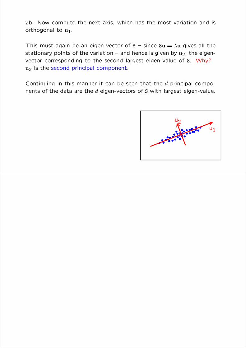
2b. Now compute the next axis, which has the most variation and is

orthogonal to u1.

This must again be an eigen-vector of S — since Su = λu gives all the

stationary points of the variation — and hence is given by u2, the eigen-

vector corresponding to the second largest eigen-value of S. Why?

u2 is the second principal component.

Continuing in this manner it can be seen that the d principal compo-

nents of the data are the d eigen-vectors of S with largest eigen-value.

u1

u2

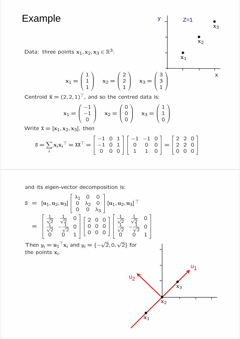
Example

Data: three points x1,x2,x3 ∈ R3:

x1 =

⎛⎜⎝ 111

⎞⎟⎠ x2 =

⎛⎜⎝ 221

⎞⎟⎠ x3 =

⎛⎜⎝ 331

⎞⎟⎠Centroid x̄ = (2,2,1)>, and so the centred data is:

x1 =

⎛⎜⎝ −1−10

⎞⎟⎠ x2 =

⎛⎜⎝ 000

⎞⎟⎠ x3 =

⎛⎜⎝ 110

⎞⎟⎠Write X = [x1,x2,x3], then

S =Xi

xixi> = XX> =

⎡⎢⎣ −1 0 1−1 0 10 0 0

⎤⎥⎦⎡⎢⎣ −1 −1 00 0 01 1 0

⎤⎥⎦ =⎡⎢⎣ 2 2 02 2 00 0 0

⎤⎥⎦

x1

x2

x3

x

y Z=1

and its eigen-vector decomposition is:

S = [u1,u2,u3]

⎡⎢⎣ λ1 0 00 λ2 00 0 λ3

⎤⎥⎦ [u1,u2,u3]>

=

⎡⎢⎢⎢⎣1√2

1√2

0

1√2− 1√

20

0 0 1

⎤⎥⎥⎥⎦⎡⎢⎣ 2 0 00 0 00 0 0

⎤⎥⎦⎡⎢⎢⎢⎣

1√2

1√2

0

1√2− 1√

20

0 0 1

⎤⎥⎥⎥⎦Then yi = u1

>xi and yi = {−√2,0,

√2} for

the points xi.

x1

x2

x3

u1

u2

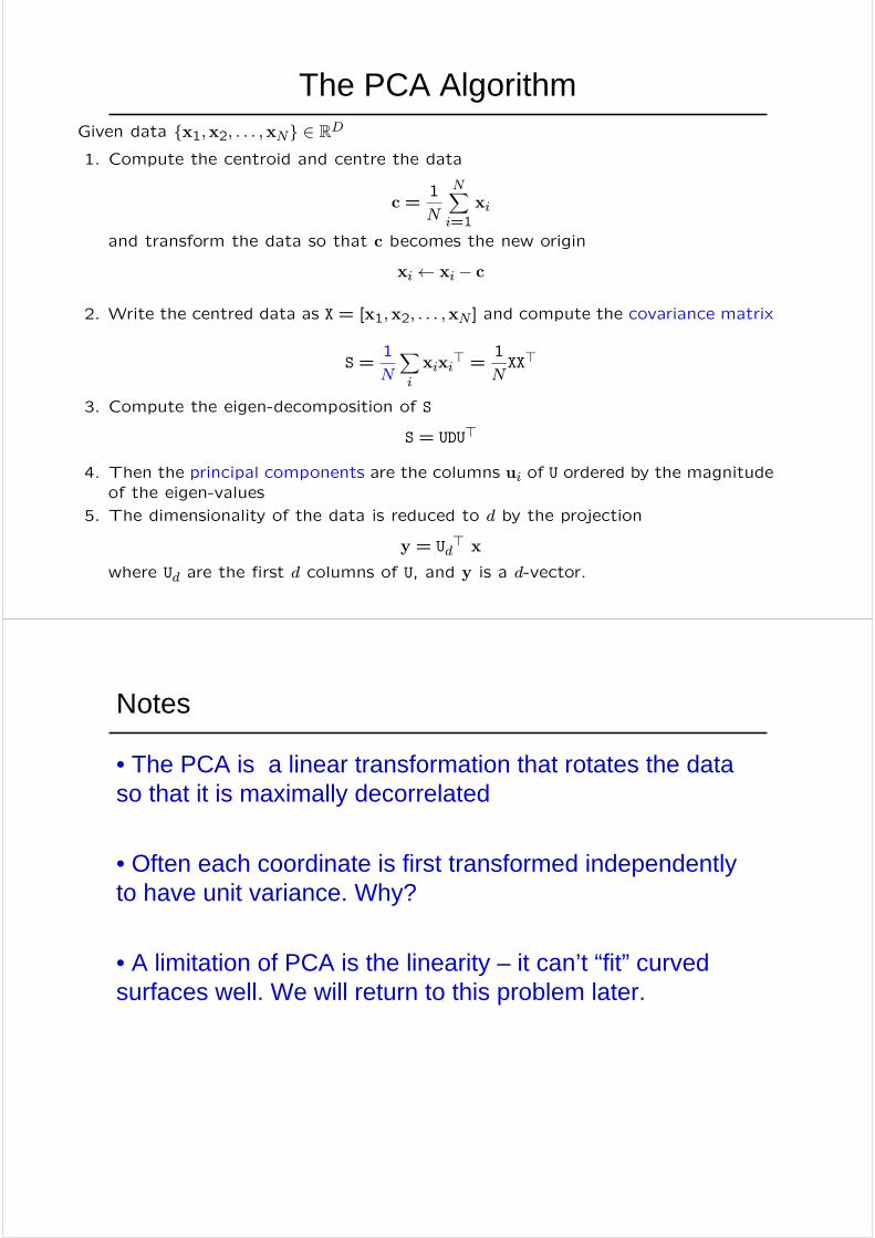
Given data {x1,x2, . . . ,xN} ∈ RD

1. Compute the centroid and centre the data

c =1

N

NXi=1

xi

and transform the data so that c becomes the new origin

xi ← xi − c

2. Write the centred data as X = [x1,x2, . . . ,xN ] and compute the covariance matrix

S =1

N

Xi

xixi> =

1

NXX>

3. Compute the eigen-decomposition of S

S = UDU>

4. Then the principal components are the columns ui of U ordered by the magnitudeof the eigen-values

5. The dimensionality of the data is reduced to d by the projection

y = Ud> x

where Ud are the first d columns of U, and y is a d-vector.

The PCA Algorithm

Notes

• The PCA is a linear transformation that rotates the data so that it is maximally decorrelated

• Often each coordinate is first transformed independently to have unit variance. Why?

• A limitation of PCA is the linearity – it can’t “fit” curved surfaces well. We will return to this problem later.

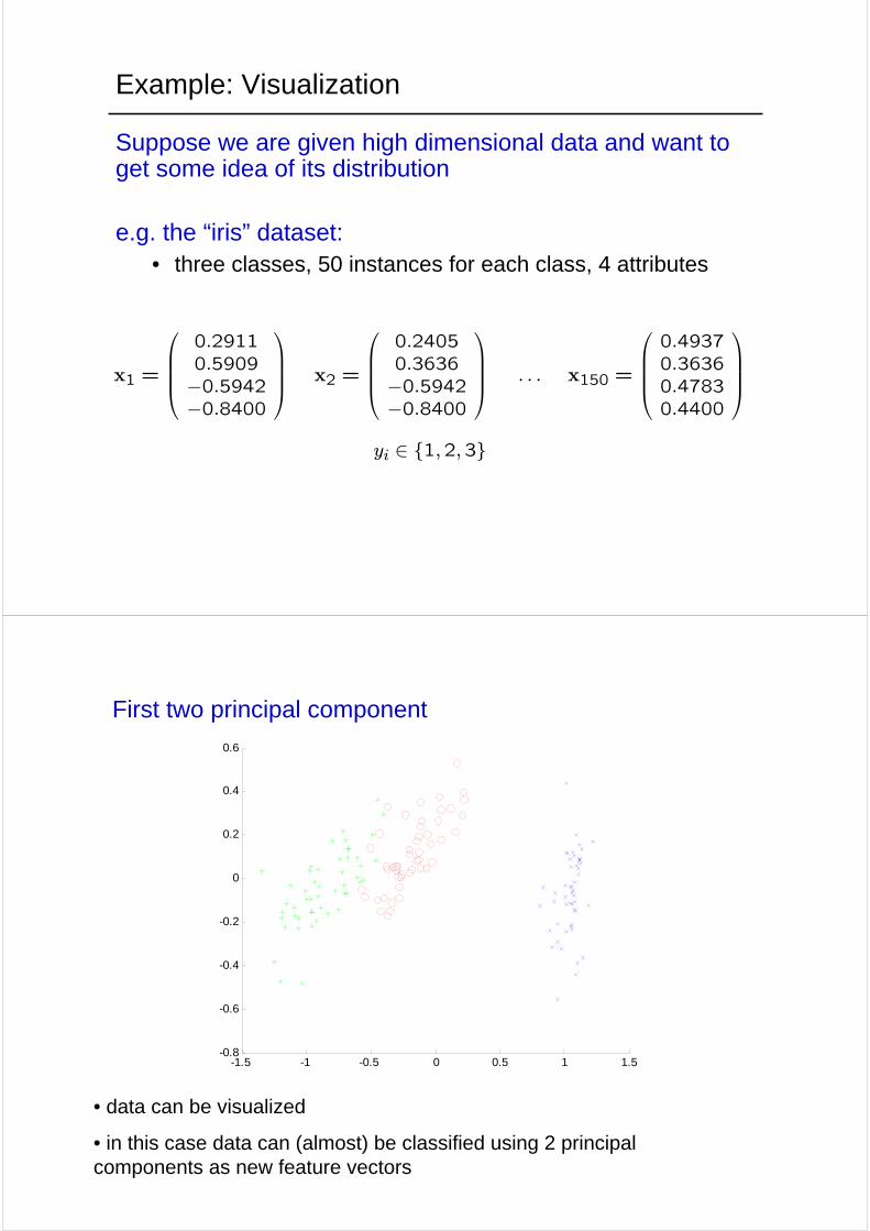
Example: Visualization

Suppose we are given high dimensional data and want to get some idea of its distribution

e.g. the “iris” dataset: • three classes, 50 instances for each class, 4 attributes

x1 =

⎛⎜⎜⎜⎝0.29110.5909−0.5942−0.8400

⎞⎟⎟⎟⎠ x2 =

⎛⎜⎜⎜⎝0.24050.3636−0.5942−0.8400

⎞⎟⎟⎟⎠ . . . x150 =

⎛⎜⎜⎜⎝0.49370.36360.47830.4400

⎞⎟⎟⎟⎠yi ∈ {1,2,3}

-1.5 -1 -0.5 0 0.5 1 1.5-0.8

-0.6

-0.4

-0.2

0

0.2

0.4

0.6

First two principal component

• data can be visualized

• in this case data can (almost) be classified using 2 principal components as new feature vectors

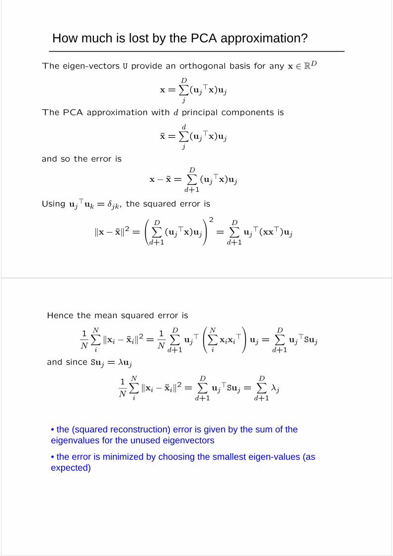
The eigen-vectors U provide an orthogonal basis for any x ∈ RD

x =DXj

(uj>x)uj

The PCA approximation with d principal components is

x̃ =dXj

(uj>x)uj

and so the error is

x− x̃ =DXd+1

(uj>x)uj

Using uj>uk = δjk, the squared error is

kx− x̃k2 =⎛⎝ DXd+1

(uj>x)uj

⎞⎠2 = DXd+1

uj>(xx>)uj

How much is lost by the PCA approximation?

Hence the mean squared error is

1

N

NXi

kxi − x̃ik2 =1

N

DXd+1

uj>⎛⎝ NXi

xixi>⎞⎠uj = DX

d+1

uj>Suj

and since Suj = λuj

1

N

NXi

kxi − x̃ik2 =DXd+1

uj>Suj =

DXd+1

λj

• the (squared reconstruction) error is given by the sum of the eigenvalues for the unused eigenvectors

• the error is minimized by choosing the smallest eigen-values (as expected)

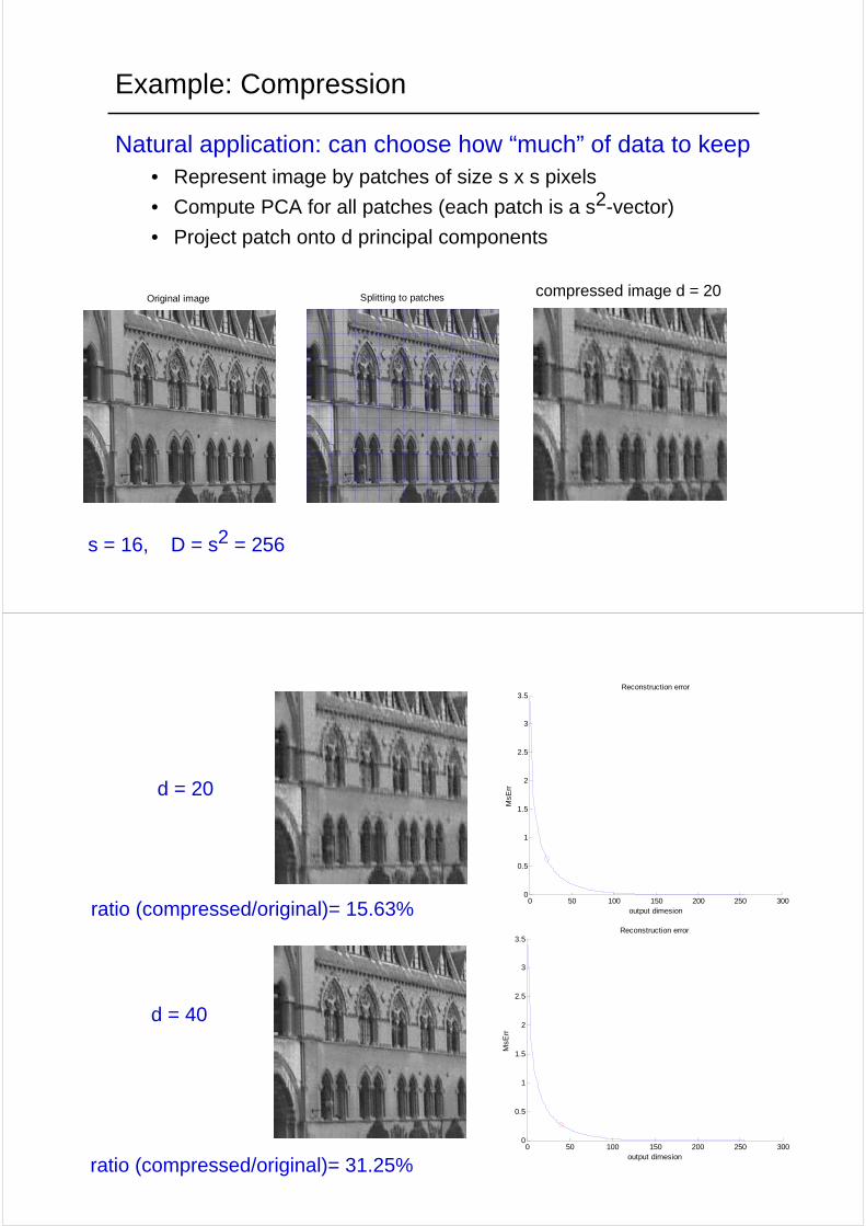
Example: Compression

Natural application: can choose how “much” of data to keep• Represent image by patches of size s x s pixels

• Compute PCA for all patches (each patch is a s2-vector)

• Project patch onto d principal components

Original image Splitting to patches

s = 16, D = s2 = 256

compressed image d = 20

0 50 100 150 200 250 3000

0.5

1

1.5

2

2.5

3

3.5Reconstruction error

output dimesion

MsE

rr

0 50 100 150 200 250 3000

0.5

1

1.5

2

2.5

3

3.5Reconstruction error

output dimesion

MsE

rr

ratio (compressed/original)= 31.25%

d = 40

ratio (compressed/original)= 15.63%

d = 20

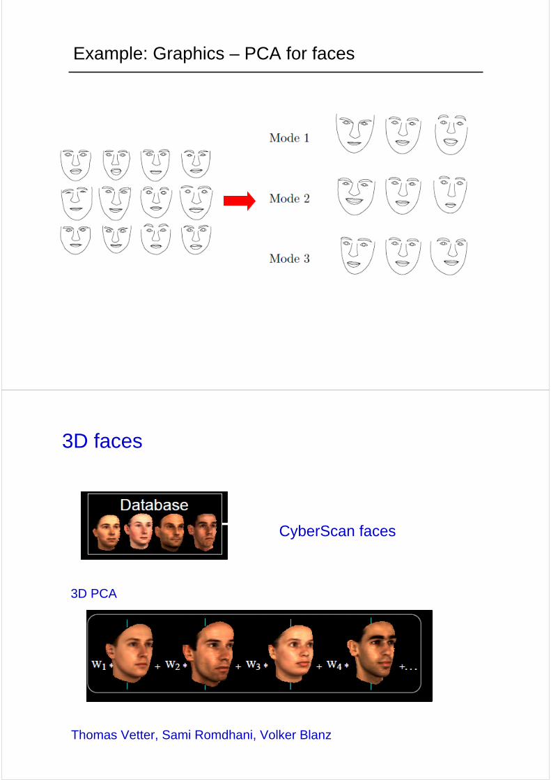
Example: Graphics – PCA for faces

3D PCA

3D faces

CyberScan faces

Thomas Vetter, Sami Romdhani, Volker Blanz

Example: 3D PCA for faces

Fitting to an image

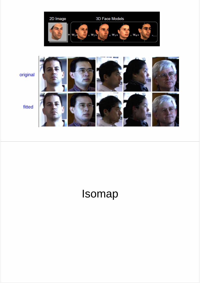
original

fitted

Isomap

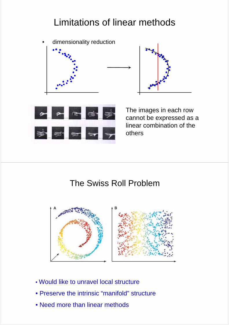
Limitations of linear methods

• dimensionality reduction

The images in each row cannot be expressed as a linear combination of the others

The Swiss Roll Problem

• Would like to unravel local structure

• Preserve the intrinsic “manifold” structure

• Need more than linear methods

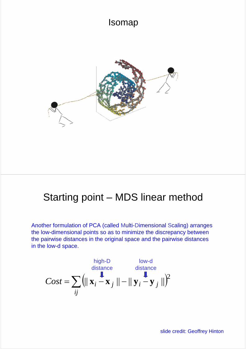
Isomap

Starting point – MDS linear method

Another formulation of PCA (called Multi-Dimensional Scaling) arranges the low-dimensional points so as to minimize the discrepancy between the pairwise distances in the original space and the pairwise distances in the low-d space.

( )2||||||||∑ −−−=ij

jijiCost yyxx

high-D distance

low-d distance

slide credit: Geoffrey Hinton

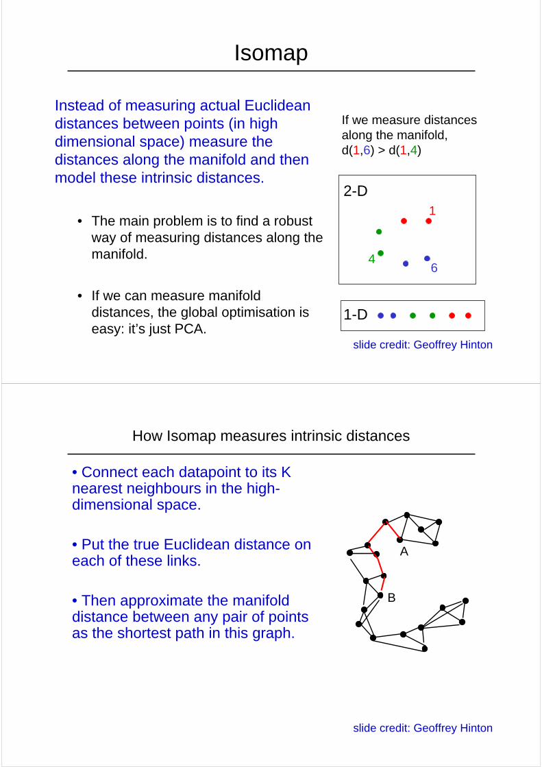
Isomap

Instead of measuring actual Euclidean distances between points (in high dimensional space) measure the distances along the manifold and then model these intrinsic distances.

• The main problem is to find a robust way of measuring distances along the manifold.

• If we can measure manifold distances, the global optimisation is easy: it’s just PCA.

2-D

1-D

If we measure distances along the manifold, d(1,6) > d(1,4)

1

46

slide credit: Geoffrey Hinton

How Isomap measures intrinsic distances

• Connect each datapoint to its K nearest neighbours in the high-dimensional space.

• Put the true Euclidean distance on each of these links.

• Then approximate the manifold distance between any pair of points as the shortest path in this graph.

A

B

slide credit: Geoffrey Hinton

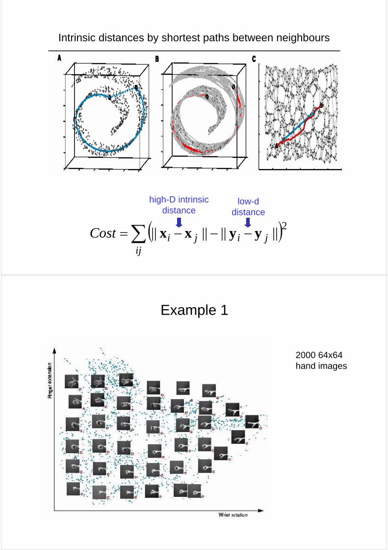
Intrinsic distances by shortest paths between neighbours

( )2||||||||∑ −−−=ij

jijiCost yyxx

high-D intrinsic distance

low-d distance

Example 1

2000 64x64 hand images

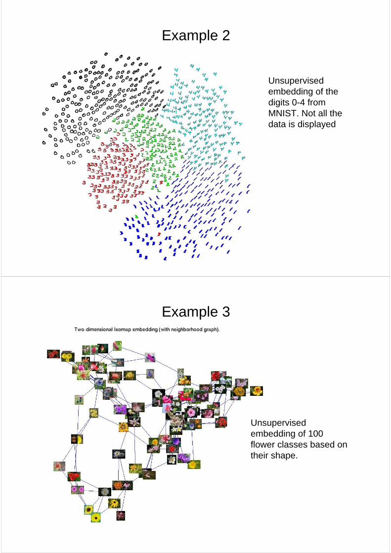
Example 2

Unsupervised embedding of the digits 0-4 from MNIST. Not all the data is displayed

Example 3

Unsupervised embedding of 100 flower classes based on their shape.

Background reading

• Bishop, chapter 12

• Other dimensionality reduction methods:

• Multi-dimensional scaling (MDS),

• Locally Linear Embedding (LLE)

• More on web page:

http://www.robots.ox.ac.uk/~az/lectures/ml