Lecture 7-Simple Linear Regression Model-Hypothesis

ACE 562, University of Illinois at Urbana-Champaign 7-1

ACE 562 Fall 2005

Lecture 7: The Simple Linear Regression Model:

Hypothesis Testing

by Professor Scott H. Irwin

Required Readings: Griffiths, Hill and Judge. "Statistical Inference II: Interval Estimation and Hypothesis Tests for the Mean of a Normal Population," Ch. 4 and "Hypothesis Testing," Section 7.2 in Learning and Practicing Econometrics


Overview Many economic problems require some basis for deciding whether a parameter of the statistical model is equal to a specified value Recall the model for household food expenditure and income,

1 2 1,...,t t ty x e t Tβ β= + + =

where yt is household food expenditure, xt is household income, and et is the error term

• An important question is whether 2 0β = or 2 0β ≠

• If 2 0β = , then there is no relationship between

household food expenditure and income, which would contradict the underlying economic model

• If 2 0β ≠ , then there is a relationship between

household food expenditure and income, presumably positive, which would be consistent with the underlying economic model


Hypothesis tests use the information about a population parameter that is contained in a sample of data to draw a conclusion about the hypothesis

• Hypothesis: statement, or conjecture, about a population parameter

• Information: least squares point estimate and

estimated standard error

• Example: Is the sample data on food expenditure and income from 40 households more consistent with 2 0β = or 2 0β ≠ ?

All hypothesis tests have four basic elements

1. A null hypothesis, H0 2. An alternative hypothesis, H1 3. A test statistic 4. A rejection region


It is helpful to consider the parallel between hypothesis testing and a jury trial, Statistical Hypothesis Test Jury Trial Null Hypothesis ⇒ Not Guilty Alternative Hypothesis ⇒

Guilty

Test Statistic ⇒ Evidence Presented in Court of Law

Rejection Region ⇒ Beyond a Reasonable Doubt

Questions:

• Why don't we conclude "Innocent" instead of "Not Guilty"?

• Why do we make "Not Guilty" the null

hypothesis in a jury trial instead of "Guilty"?

• Where is the element of chance in both procedures?

Hint: If hypothesis testing seems confusing, remembering the analogy to a jury trial may be helpful


Null Hypothesis

• Belief we maintain until convinced by the sample evidence that it is not true

• Denoted H0 ("h-naught")

Alternative Hypothesis

• Logical alternative to H0 that is accepted if the null hypothesis is rejected

• Denoted H1 or Ha

Alternative Hypothesis Setups

Hill, Griffiths, Judge Conventional

0 2

1 2

: 0: 0

HH

ββ

=≠

0 2

1 2

: 0: 0

HH

ββ

=≠

0 2

1 2

: 0: 0

HH

ββ

=>

0 2

1 2

: 0: 0

HH

ββ

≤>

0 2

1 2

: 0: 0

HH

ββ

=<

0 2

1 2

: 0: 0

HH

ββ

≥<


Sampling Theory and Hypothesis Testing The estimator 2b has a sampling distribution with mean 2β and 2var( )b

• The estimate for a particular sample is generated by blindly reaching into this sampling distribution and selecting one value

If 0 2: 0H β = is true,

• Sampling theory implies that 2b can take on any value from to −∞ + ∞

If 0 2: 0H β = is not true,

• Sampling theory implies that 2b can take on any value from to −∞ + ∞

Implication: It will never be possible to conclude absolutely that one hypothesis is right and one is wrong, because every possible value of 2b is theoretically consistent with both hypotheses! Must resort to probabilistic reasoning


Test Statistic Sample information about the validity of the null hypothesis is embodied in the sample value of a test statistic

• Test statistic is a random variable

• Based on sample value of test statistic, will reject or not reject null hypothesis

In the previous section, we discussed the following standardized random variable,

2

2 2

2ˆvar( )bbt

bβ−

=

Assuming the linear statistical model is correct, the random variable

2bt captures the information necessary to conduct hypothesis tests

• 2b , the point estimate of 2β

• 2 2ˆ ˆvar( ) ( )b se b= , the estimated standard error of the sampling distribution of 2b


Two more important characteristics of a test statistic,

• The sampling distribution of the test statistic is "known" under the null hypothesis

• The sampling distribution of the test statistic

under the alternative hypothesis is "something else"

In the previous section, we derived the sampling distribution of

2bt ,

2

2 22

2

~ˆvar( )b T

bt tbβ

−−

=

Now consider the following hypotheses,

0 2

1 2

: 0: 0

HH

ββ

=≠

If the null hypothesis is true, and 2 0β = , then it must also be true that,

2

2 22

2 2

0 ~ˆ ˆvar( ) var( )b T

b bt tb b −

−= =



If the null hypothesis is not true, then 2

2ˆvar( )b

b

is not distributed as a t-distribution For example, what if 2 1β = is true, rather than

2 0β = ? In this case,

2

22

2

1 ~ˆvar( )b T

bt tb −

−=

and 2

2ˆvar( )b

b is not ~ tT-2

The reason is that in its formation, the numerator of the above equation is not standard normal, N(0,1)

• Numerator must be N(0,1) in order to derive the t-distribution

• Instead the numerator is N(1,1)

• See the derivation of

2bt in the previous section for the full details


Rejection Region Foundation of hypothesis testing is the sampling theory result that under the assumptions of the linear statistical model,

2

2 22

2

~ˆvar( )b T

bt tbβ

−−

=

We now ask whether a particular sample value of

2bt is more consistent with a sampling distribution centered at the null hypothesis value for 2β or the alternative hypothesis To do this, we set up a rejection region for the test statistic

2bt , • A set of test statistic values that have a low

probability of occurring when the null hypothesis is true

• If a sample value of

2bt falls in the rejection region we reject the null hypothesis

• If a sample value of

2bt does not fall in the rejection region we do not reject the null hypothesis


Consider again the following hypotheses,

0 2

1 2

: 0: 0

HH

ββ

=≠

If the null hypothesis is true, and 2 0β = , then we know that,

2

2 22

2 2

0 ~ˆ ˆvar( ) var( )b T

b bt tb b −

−= =

The null hypothesis will be rejected only if an unusually "small" or "large" value of

2bt is observed "Small" and "large" are determined by α

• Tail probabilities that correspond to "small" or "large" values of

2bt

• Level of significance of the test

• α typically set to 0.01, 0.05, or 0.10


Once α is set, the rejection region is found by generating critical values such that,

2 2[ ] [ ]2T c T cP t t P t t α

− − −≥ = ≤ =

or,

2 2[ ] [ ]T c T cP t t P t t α− − −≥ + ≤ =

and,

2[ ] 1c T cP t t t α− −≤ ≤ = − We can now state a formal set of rejection rules for "two-tailed" hypothesis tests,

• If the sample estimate of the test statistic falls in the rejection region,

2b ct t−≤ or 2b ct t≥ , reject the

null hypothesis and accept the alternative

• If the sample estimate of the test statistic falls in the non-rejection region,

2c b ct t t− < < , do not reject the null hypothesis and reject the alternative



Hypothesis Test in the Food Expenditure Example Again, the model for household food expenditure and income is,

1 2 1,...,t t ty x e t Tβ β= + + =

where yt is household food expenditure, xt is household income, and et is the error term Let's first consider the following null and alternative hypotheses,

0 2

1 2

: 0: 0

HH

ββ

=≠

To test these hypotheses, we will use the sample information summarized as follows,

ˆ 7.3832 0.2323(4.0080) (0.0553) ( . .)

t ty xs e

= +

Under the null hypothesis, the test statistic is,

2

22

2

~ˆvar( )b Tbt t

b −=


After the hypotheses and test statistic have been stated, the following steps are necessary,

1. Select the level of significance, in this example we will assume 0.05α =

• For 38 degrees of freedom (T-2), the critical t-

values at this level of significance are -2.024 and 2.024

2. Determine the rejection rule

• If the sample estimate of the test statistic falls in

the rejection region, 2

2.024bt ≤ − or 2

2.024bt ≥ , reject the null hypothesis and accept the alternative


the non-rejection region, 2

2.024 2.024bt− < < , do not reject the null hypothesis and reject the alternative

3. Compute the sample estimate of the test statistic

2

2

2

0.2323 4.200.055ˆvar( )b

btb

= = =


4. Compare the sample estimate of the test statistic to the rejection rules

• Since 2

( 4.20) ( 2.024)b ct t= > = , we reject the null hypothesis and accept the alternative hypothesis

• "Sample information indicates a statistically

significant relationship between food expenditure and income"



Sample Regression Output from Excel

SUMMARY OUTPUT

Regression StatisticsMultiple R 0.563096017R Square 0.317077125Adjusted R Square 0.29910547Standard Error 6.844922384Observations 40

ANOVAdf SS MS F Significance F

Regression 1 826.6352172 826.6352 17.64318 0.000155136Residual 38 1780.412573 46.85296Total 39 2607.04779

Coefficients Standard Error t Stat P-value Lower 95% Upper 95%Intercept 7.383217543 4.008356335 1.841956 0.073296 -0.731275911 15.497711X Variable 1 0.23225333 0.055293429 4.200378 0.000155 0.120317631 0.34418903


Up to this point, we have only considered hypotheses about the slope parameter The procedure for setting up and testing hypotheses about the intercept parameter closely parallel the procedure for the slope Consider the following null and alternative hypotheses,

0 1

1 1

: 0: 0

HH

ββ

=≠

To test these hypotheses, we again will use the sample information summarized as follows,

ˆ 7.3832 0.2323(4.0080) (0.0553) ( . .)

t ty xs e

= +

Under the null hypothesis, the test statistic is,

1

12

1

~ˆvar( )b Tbt t

b −=


After the hypotheses and test statistic have been stated, the following steps are necessary,

1. Select the level of significance, in this example we will assume 0.05α =

• For 38 degrees of freedom (T-2), the critical t-values at this level of significance are -2.024 and 2.024

2. Determine the rejection rule


the rejection region, 1

2.024bt ≤ − or 1

2.024bt ≥ , reject the null hypothesis and accept the alternative


the non-rejection region, 1

2.024 2.024bt− < < , do not reject the null hypothesis and reject the alternative

3. Compute the sample estimate of the test statistic

1

1

1

7.3832 1.844.0084ˆvar( )b

btb

= = =


4. Compare the sample estimate of the test statistic to the rejection rules

• Since 1

( 2.024) ( 1.84) ( 2.024)c b ct t t− = − < = < = , we do not reject the null hypothesis and reject the alternative hypothesis


insignificant intercept in the relationship between food expenditure and income"


Interpreting Hypothesis Test Results In the previous section, we rejected the null hypothesis that 2 0β = This can be interpreted in terms of the sample information and the data-generating process (statistical model)

• The null hypothesis is not compatible with the sample data and we go with our point estimate

2 0.2323b =

• The linear statistical model, 1 2t t ty x eβ β= + + , more appropriately describes the data-generating process than the constant mean model,

1t ty eβ= + In the previous section, we did not reject the null hypothesis that 1 0β =

• Notice that we did not say that we accept the null hypothesis that 1 0β =

• There is a subtle, but important distinction

between not rejecting and accepting a null hypothesis


To see this distinction, consider the following two sets of hypotheses about the intercept in the food expenditure statistical model,

0 1

1 1

: 0: 0

HH

ββ

=≠

0 1

1 1

: 1: 1

HH

ββ

=≠

When the null is 1 0β = ,

1

1

1

0 7.3832 1.844.0084ˆvar( )b

btb

−= = =

and we do not reject this null When the null is 1 1β = ,

1

1

1

1 6.3832 1.594.0084ˆvar( )b

btb

−= = =

and we do not reject this null either

Which null hypothesis is “true”?


The answer is that both null hypotheses are "true" in the sense that the sample information is consistent with both null hypotheses Basic precept of hypothesis testing

• Finding a value of the test statistic in the non-rejection region does not make the null hypothesis true

• When testing a null hypothesis we should

always be aware that another null hypothesis (particularly when the null values are close) may be equally compatible with the data

…just as a court pronounces a verdict as “not guilty” rather than “innocent,” so the conclusion of a statistical test is “do not reject” rather than “accept.”

---Jan Kmenta


Hypothesis Testing and Confidence Intervals It is possible to conduct two-tailed hypothesis tests using confidence intervals To see this, note that the non-rejection region for the hypothesis considered earlier is

2c b ct t t− < < which can be re-arranged as follows,

2 2

2ˆ ( )c cbt tse b

β−

−< <

2 2 2 2 2ˆ ˆ( ) ( )c cb t se b b t se bβ−− ⋅ < < + ⋅

The last result has the same endpoints as a (1 ) 100%α− ⋅ confidence interval estimate of 2β

• Fail to reject if the null hypothesis value, e.g. 2 0β = , is within the endpoints of the confidence

interval

• Reject if the null hypothesis value, e.g. 2 0β = , is outside the endpoints of the confidence interval


Food Expenditure Example Let's first consider the following null and alternative hypotheses,

0 2

1 2

: 0: 0

HH

ββ

=≠

As shown in Lecture 6, the 95% confidence interval estimate for 2β is,

0.2323 2.2024 0.00306± ⋅ or,

2(0.12 0.34)β≤ ≤ Since 2 0β = is outside the endpoints of the confidence interval, we reject the null hypothesis and accept the alternative hypothesis


significant relationship between food expenditure and income"

• Same conclusion as reached with “conventional”

hypothesis testing procedures


Type I and II Errors Whenever we reject or don't reject a null hypothesis, there is the chance of making a mistake For comparison, there are two ways of making a correct decision,

• The null hypothesis is false and we decide to reject it

• The null hypothesis is true and we decide not

to reject it There are two ways of making an incorrect decision,

• The null hypothesis is true and we decide to reject it (Type I error)

• The null hypothesis is false and we decide not

to reject it (Type II error)


Whenever we reject a null hypothesis we risk a Type I error

• The probability of a Type I error is α , the level of significance of the test

• We will reject a true null hypothesis with a

probability equal to α

• We control the probability of a Type I error by choosing the level of significance

• If a Type I error is costly, we will want to

make α small (e.g. 0.05, 0.01) We risk a Type II error whenever we do not reject a null hypothesis

• Probability of a Type II error is not a single value, as it depends on the true but unknown value of the parameter in question

• Probability of a Type II error is not under our

control





What do we know about Type II error?

• Probability of a Type II error varies inversely with the level of significance, α

• The closer the true value of the parameter to

the hypothesized parameter value under 0H , the higher the probability of a Type II error (see previous figure)

• For a given α , the probability of a Type II

error decreases as T increases


Hypothesis Testing: Putting It All Together The logic of hypothesis testing often can be difficult to understand and bewildering The key is to understand that there are four inter-related components that influence hypothesis test results

1. Sample size (T ): the number of observations available for the test

2. Significance level (α ): the probability that the

observed test result is due to chance

3. Power (1 δ− ): The probability that a true non-zero relationship will be detected

4. Magnitude ( 2β ): the size of the relationship

relative to the noise in the test There is a relationship between the four components:

In fact, given values for three of the components, it is possible to compute the fourth!


The goal in conducting hypothesis tests is to balance the four components in order to maximize our ability to detect a relationship if one exists, given data, financial, logistical, legal or other constraints For a given test, some components will be easier to manipulate than others

• Sample size may be fixed due to data availability

• Economic magnitude of a relationship may be small during certain time periods

• In applied econometric research, we will often

only have control over sample size and the significance level


0 2: 0H β = (null hypothesis) is true

1 2: 0H β ≠ (alternative hypothesis) is false In reality...

There is no relationship

Slope is zero

Our theory is wrong

0 2: 0H β = (null hypothesis) is false

1 2: 0H β ≠ (alternative hypothesis) is true

In reality... There is a relationship Slope is not zero Our theory is correct

We do not reject the null hypothesis (H0) We reject the alternative hypothesis (H1)

We say...

"There is no evidence of a relationship" "Sample evidence is consistent with null hypothesis" "Our theory is inconsistent with sample evidence"

1 α−

(e.g., 0.95)

THE CONFIDENCE LEVEL

The probability of saying there is no relationship when in fact there is none

The probability of correctly not confirming our theory

95 times out of 100 when there is no relationship, we’ll say there is none

δ

(e.g., 0.20)

TYPE II ERROR

The probability of saying there is no relationship when in fact there is one r

The probability of not confirming our theory when it’s true

20 times out of 100, when there is a relationship, we’ll say there isn’t

We reject the null hypothesis (H0) We accept the alternative hypothesis (H1)

We say...

"There is evidence of a relationship"

“Sample evidence is inconsistent with null hypothesis" "Our theory is consistent with sample evidence"

α

(e.g., 0.05)

THE SIGNIFICANCE LEVEL & TYPE I ERROR

The probability of saying there is a relationship when in fact there is none

The probability of confirming our theory incorrectly

5 times out of 100, when there is no relationship, we’ll say there is one

We should keep this small when we can’t risk a wrong conclusion

1 δ−

(e.g., 0.80)

POWER

The probability of saying that there is a relationship when in fact there is one rrr

The probability of confirming our theory correctly g

80 times out of 100, when there is a relationship, we’ll say there is one

We generally want this to be as large as possible

The Statistical Inference Decision Matrix

Adapted from: Trochim, William M. Research Methods Knowledge Base. http://trochim.human.cornell.edu/kb/index.htm.


Hypothetical Example of the Tradeoff between Power and Significance Level (all else held constant)

0.00

0.10

0.20

0.30

0.40

0.50

0.60

0.70

0.80

0.90

1.00

0.00 0.02 0.04 0.06 0.08 0.10 0.12 0.14 0.16Significance Level

Pow

er


Terminology Highlights Often discuss significance level (α ) and power (1 δ− ) of hypothesis tests using the terms "higher" and "lower" Might be interested in the advantages of a higher or lower significance level (α ) in an econometric study (which is directly controlled by the researcher)

• Higher α -level [ ]0.05 0.10α α= → = means an increase in the chance of a Type I error

• Lower α -level [ ]0.10 0.01α α= → = means a

decrease in the chance of a Type I error and a more “rigorous” test

Also might be interested in the advantages of higher or lower power (1 δ− ) in an econometric study (which is not directly controlled by the researcher)

• Higher 1 δ− [ ]0.80 0.50δ δ= → = means an decrease in the chance of a Type II error

• Lower 1 δ− [ ]0.20 0.40δ δ= → = means an

increase in the chance of a Type II error


Examples of Possible Statements Based on the Hypothesis Testing Decision Matrix

• The lower the significance level of a test, the lower the power of a test; the higher the significance level of a test, the higher the power

• The higher the power of a test, the higher the

significance level; the lower the power, the lower the significance level

• The higher the significance level, the more likely

it is that you will make a Type I error (reject the null when it’s true) and the less likely you will make a Type II error (reject the alternative when it’s true)

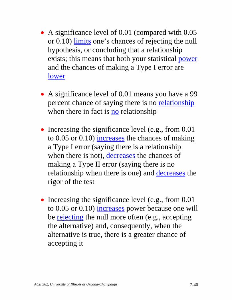
• A significance level of 0.01 (compared with 0.05

or 0.10) means a researcher is being relatively careful; they are only willing to risk being wrong (rejecting the null when it’s true) 1 in a 100 times


• A significance level of 0.01 (compared with 0.05 or 0.10) limits one’s chances of rejecting the null hypothesis, or concluding that a relationship exists; this means that both your statistical power and the chances of making a Type I error are lower

• A significance level of 0.01 means you have a 99

percent chance of saying there is no relationship when there in fact is no relationship

• Increasing the significance level (e.g., from 0.01

to 0.05 or 0.10) increases the chances of making a Type I error (saying there is a relationship when there is not), decreases the chances of making a Type II error (saying there is no relationship when there is one) and decreases the rigor of the test

• Increasing the significance level (e.g., from 0.01

to 0.05 or 0.10) increases power because one will be rejecting the null more often (e.g., accepting the alternative) and, consequently, when the alternative is true, there is a greater chance of accepting it


p-value of a Hypothesis Test It has become common in recent years to report the p-value of a hypothesis test p-value of a test statistic is simply the actual probability that a test statistic is greater than or equal to the absolute value of the sample statistic

• Previous definition applies only to two-tailed tests

If the following null and alternative hypotheses are specified,

0 2

1 2

: 0: 0

HH

ββ

=≠

Then the p-value of the test statistic is,

( )22T bpr t t− ≥ or

( ) ( )2 22 2T b T bpr t t pr t t− −≤ − + ≥


We can use the p-value to conduct an hypothesis test,

• Rejection rule: When the p-value is smaller than α , reject the null hypothesis

• Handy rule, can determine results without

looking up critical values Reporting of p-values is done so that a reader may conduct their own hypothesis tests based on a different α level than that used by the researcher


Sample Regression Output from Excel

SUMMARY OUTPUT

Regression StatisticsMultiple R 0.563096017R Square 0.317077125Adjusted R Square 0.29910547Standard Error 6.844922384Observations 40

ANOVAdf SS MS F Significance F

Regression 1 826.6352172 826.6352 17.64318 0.000155136Residual 38 1780.412573 46.85296Total 39 2607.04779

Coefficients Standard Error t Stat P-value Lower 95% Upper 95%Intercept 7.383217543 4.008356335 1.841956 0.073296 -0.731275911 15.497711X Variable 1 0.23225333 0.055293429 4.200378 0.000155 0.120317631 0.34418903



A More General Null Hypothesis Zero is not the only null hypothesis of interest A more general form,

0 1

1 1

::

H kH k

ββ

=≠

0 2

1 2

::

H kH k

ββ

=≠

where k is any constant The corresponding test statistics are,

1

1

1ˆvar( )bb kt

b−

= 2

2

2ˆvar( )bb kt

b−

=

One-Tailed Tests We have focused so far on "two-tailed" hypothesis tests "One-tailed" tests are also quite common in economic research


For a "right-tail" test,

• Hypotheses: 0 2

1 2

: 0: 0

HH

ββ

≤>

• Test statistic: 2

22

2

~ˆvar( )b Tbt t

b −=

• Rejection region:

2b ct t≥

• p-value: ( )22T bpr t t− ≥ For a "left-tail" test,

• Hypotheses: 0 2

1 2

: 0: 0

HH

ββ

≥<

• Test statistic: 2

22

2

~ˆvar( )b Tbt t

b −=

• Rejection region:

2b ct t−≤

• p-value: ( )22T bpr t t− ≤ −



Stating Null and Alternative Hypotheses The previous discussion shows that a statistical test procedure cannot prove the truth of a null hypothesis

• Failure to reject a null hypothesis proves only that the sample data are compatible with the null

• When a null hypothesis is rejected, usually there

is only a small probability (α ) of the rejection being incorrect

⇒Rejecting a null hypothesis typically is

"stronger" than failing to reject it Consequently, the null hypothesis is usually stated so that rejection implies our economic model is correct Food Expenditure Example

0 2

1 2

: 0: 0

HH

ββ

=

≠

Final note: Hypotheses must be established before carrying out investigation


Statistical Significance vs. Economic Significance When a null, say, 1jβ = , is specified, the likely intent is that jβ is close to 1, so close that for all practical purposes it may be treated as if it were 1. But whether 1.1 is “practically the same as” 1.0 is a matter of economics, not of statistics. One cannot resolve the matter by relying on a hypothesis test, because the test statistic ˆ( 1) /

jj bt b σ= − measures the estimated coefficient in standard error units, which are not meaningful units in which to measure the economic parameter. It may be a good idea to reserve the term “significance” for the statistical concept, adopting “substantial” for the economic concept.

---Goldberger

• Conflict between economic and statistical significance may be especially noticeable when the sample size becomes very large

• In these cases, it is often easy to reject null

hypotheses simply because the large sample size dramatically decreases standard errors


Example Suppose the CEO of the supermarket chain plans a certain course of action if 2 0β ≠ Furthermore suppose a large sample, say 10,000 observations, is collected from which we obtain the estimate b2 = 0.0001 with 2ˆ ( )= 0.00001se b , yielding the t-statistic t = 10.0 We would reject the null hypothesis that 2 0β = and accept the alternative that 2 0β ≠ , and conclude that b2 = 0.0001 is statistically different from zero However, 0.0001 may not be “economically” different from zero, as this depends critically on the decision environment

• Units of y and x

• Economic impact of a one-unit change in x The CEO’s decision may be more affected by economic significance


Recommended Reading: McCloskey, D. N. and S. T. Ziliak. "The Standard Error of Regressions." Journal of Economic Literature, 34(1996): 97-114.

• We here examine the alarming hypothesis that ordinary usage in economics takes statistical significance to be the same as economic significance.

• The question “How large is large?” requires

thinking about what coefficients would be judged large or small in terms of the present conversation of the science. It requires thinking more rigorously about data…

Documents

Lecture 7-Simple Linear Regression Model-Hypothesis