Embed Size (px)
Citation preview
Probability IntroducationProbabilistic Graphical Models
Lecture 7: PGM — Representation
Qinfeng (Javen) Shi
8 September 2014
Intro. to Stats. Machine LearningCOMP SCI 4401/7401
Qinfeng (Javen) Shi Lecture 7: PGM — Representation
Probability IntroducationProbabilistic Graphical Models
Table of Contents I
1 Probability IntroducationProbability spaceConditional probabilityRandom Variables and DistributionsIndependence and conditional independence
2 Probabilistic Graphical ModelsHistory and booksRepresentationsFactorisationIndependences
Qinfeng (Javen) Shi Lecture 7: PGM — Representation
Probability IntroducationProbabilistic Graphical Models
Probability spaceConditional probabilityRandom Variables and DistributionsIndependence and conditional independence
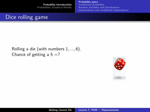
Dice rolling game
Rolling a die (with numbers 1, ..., 6).Chance of getting a 5 =?
1/6Chance of getting a 5 or 4 =?2/6
Qinfeng (Javen) Shi Lecture 7: PGM — Representation

Probability IntroducationProbabilistic Graphical Models
Probability spaceConditional probabilityRandom Variables and DistributionsIndependence and conditional independence
Dice rolling game
Rolling a die (with numbers 1, ..., 6).Chance of getting a 5 =?1/6Chance of getting a 5 or 4 =?
2/6
Qinfeng (Javen) Shi Lecture 7: PGM — Representation
Probability IntroducationProbabilistic Graphical Models
Probability spaceConditional probabilityRandom Variables and DistributionsIndependence and conditional independence
Dice rolling game
Rolling a die (with numbers 1, ..., 6).Chance of getting a 5 =?1/6Chance of getting a 5 or 4 =?2/6
Qinfeng (Javen) Shi Lecture 7: PGM — Representation
Probability IntroducationProbabilistic Graphical Models
Probability spaceConditional probabilityRandom Variables and DistributionsIndependence and conditional independence
Events and confidence
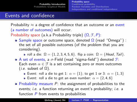
Probability ≈ a degree of confidence that an outcome or an event(a number of outcomes) will occur.Probability space (a.k.a Probability triple) (Ω,F,P):
Sample space or outcome space, denoted Ω (read “Omega”) :the set of all possible outcomes (of the problem that you areconsidering).
roll a die: Ω = 1, 2, 3, 4, 5, 6. flip a coin: Ω = Head ,Tail.A set of events, a σ-Field (read “sigma-field”) denoted F:Each even α ∈ F is a set containing zero or more outcomes(i.e. subset of Ω).
Event: roll a die to get 1: α = 1; to get 1 or 3: α = 1, 3Event: roll a die to get an even number: α = 2, 4, 6
Probability measure P: the assignment of probabilities to theevents; i.e. a function returning an event’s probability; i.e. afunction P from events to probabilities
Qinfeng (Javen) Shi Lecture 7: PGM — Representation
Probability IntroducationProbabilistic Graphical Models
Probability spaceConditional probabilityRandom Variables and DistributionsIndependence and conditional independence
Probability measure
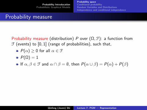
Probability measure (distribution) P over (Ω,F): a function fromF (events) to [0, 1] (range of probabilities), such that,
P(α) ≥ 0 for all α ∈ F
P(Ω) = 1
If α, β ∈ F and α ∩ β = ∅, then P(α ∪ β) = P(α) + P(β)
⇓P(∅) = 0
P(α ∪ β) = P(α) + P(β)− P(α ∩ β)
Qinfeng (Javen) Shi Lecture 7: PGM — Representation
Probability IntroducationProbabilistic Graphical Models
Probability spaceConditional probabilityRandom Variables and DistributionsIndependence and conditional independence
Probability measure
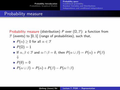
Probability measure (distribution) P over (Ω,F): a function fromF (events) to [0, 1] (range of probabilities), such that,
P(α) ≥ 0 for all α ∈ F
P(Ω) = 1
If α, β ∈ F and α ∩ β = ∅, then P(α ∪ β) = P(α) + P(β)⇓P(∅) = 0
P(α ∪ β) = P(α) + P(β)− P(α ∩ β)
Qinfeng (Javen) Shi Lecture 7: PGM — Representation
Probability IntroducationProbabilistic Graphical Models
Probability spaceConditional probabilityRandom Variables and DistributionsIndependence and conditional independence
Interpretations of Probability
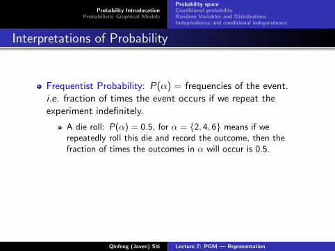
Frequentist Probability: P(α) = frequencies of the event.i.e. fraction of times the event occurs if we repeat theexperiment indefinitely.
A die roll: P(α) = 0.5, for α = 2, 4, 6 means if werepeatedly roll this die and record the outcome, then thefraction of times the outcomes in α will occur is 0.5.
Problem: non-repeatable event e.g. “it will rain tomorrowmorning” (tmr morning happens exactly once, can’t repeat).
Subjective Probability: P(α) = one’s own degree of beliefthat the event α will occur.
Qinfeng (Javen) Shi Lecture 7: PGM — Representation
Probability IntroducationProbabilistic Graphical Models
Probability spaceConditional probabilityRandom Variables and DistributionsIndependence and conditional independence
Interpretations of Probability
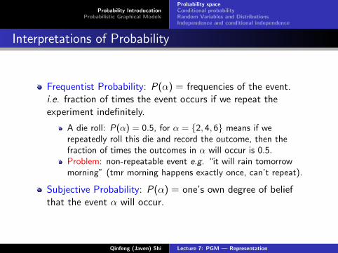
Frequentist Probability: P(α) = frequencies of the event.i.e. fraction of times the event occurs if we repeat theexperiment indefinitely.
A die roll: P(α) = 0.5, for α = 2, 4, 6 means if werepeatedly roll this die and record the outcome, then thefraction of times the outcomes in α will occur is 0.5.Problem: non-repeatable event e.g. “it will rain tomorrowmorning” (tmr morning happens exactly once, can’t repeat).
Subjective Probability: P(α) = one’s own degree of beliefthat the event α will occur.
Qinfeng (Javen) Shi Lecture 7: PGM — Representation
Probability IntroducationProbabilistic Graphical Models
Probability spaceConditional probabilityRandom Variables and DistributionsIndependence and conditional independence
Conditional probability
Event α: “students with grade A”Event β: “students with high intelligence”Event α ∩ β: “students with grade A and high intelligence”
Question: how do we update the our beliefs given new evidence?e.g. suppose we learn that a student has received the grade A,what does that tell us about the person’s intelligence?
Answer: Conditional probability.Conditional probability of β given α is defined as
P(β|α) =P(α ∩ β)
P(α)
Qinfeng (Javen) Shi Lecture 7: PGM — Representation
Probability IntroducationProbabilistic Graphical Models
Probability spaceConditional probabilityRandom Variables and DistributionsIndependence and conditional independence
Chain rule and Bayes’ rule
Chain rule: P(α ∩ β) = P(α)P(β|α)More generally,P(α1 ∩ ... ∩ αk) = P(α1)P(α2|α1) · · ·P(αk |α1 ∩ ... ∩ αk−1)
Bayes’ rule:
P(α|β) =P(β|α)P(α)
P(β)
Qinfeng (Javen) Shi Lecture 7: PGM — Representation
Probability IntroducationProbabilistic Graphical Models
Probability spaceConditional probabilityRandom Variables and DistributionsIndependence and conditional independence
Random Variables
Assigning probabilities to events is intuitive.
Assigning probabilities to attributes (of the outcome) takingvarious values might be more convenient.
a patient’s attributes such “Age”, “Gender” and “Smokinghistory” ...“Age = 10”, “Age = 50”, ..., “Gender = male”,“Gender =female”
a student’s attributes “Grade”, “Intelligence”, “Gender” ...
P(Grade = A) = the probability that a student gets a grade of A.
Qinfeng (Javen) Shi Lecture 7: PGM — Representation
Probability IntroducationProbabilistic Graphical Models
Probability spaceConditional probabilityRandom Variables and DistributionsIndependence and conditional independence
Random Variables
A random variable, such as Grade, is a function that associateswith each outcome in Ω a value. e.g. Grade is defined by afunction fGrade that maps each person to his or her grade (say, oneof A, B, C)
Grade = A is a shorthand for the event ω ∈ Ω : fGrade(ω) = A
Intelligence = high a shorthand for the eventω ∈ Ω : fIntelligence(ω) = high
Qinfeng (Javen) Shi Lecture 7: PGM — Representation
Probability IntroducationProbabilistic Graphical Models
Probability spaceConditional probabilityRandom Variables and DistributionsIndependence and conditional independence
Random Variables
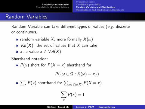
Random Variable can take different types of values (e.g. discreteor continuous.
random variable X , more formally X (ω)
Val(X ): the set of values that X can take
x : a value x ∈ Val(X )
Shorthand notation:
P(x) short for P(X = x) shorthand for
P(ω ∈ Ω : X (ω) = x)∑x P(x) shorthand for
∑x∈Val(X ) P(X = x)∑
x
P(x) = 1
Qinfeng (Javen) Shi Lecture 7: PGM — Representation
Probability IntroducationProbabilistic Graphical Models
Probability spaceConditional probabilityRandom Variables and DistributionsIndependence and conditional independence
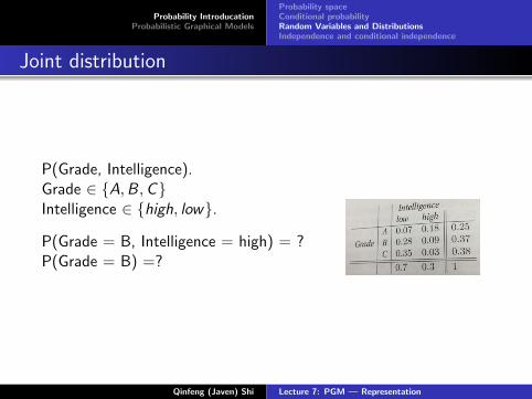
Joint distribution
P(Grade, Intelligence).Grade ∈ A,B,CIntelligence ∈ high, low.
P(Grade = B, Intelligence = high) = ?P(Grade = B) =?
Qinfeng (Javen) Shi Lecture 7: PGM — Representation
Probability IntroducationProbabilistic Graphical Models
Probability spaceConditional probabilityRandom Variables and DistributionsIndependence and conditional independence
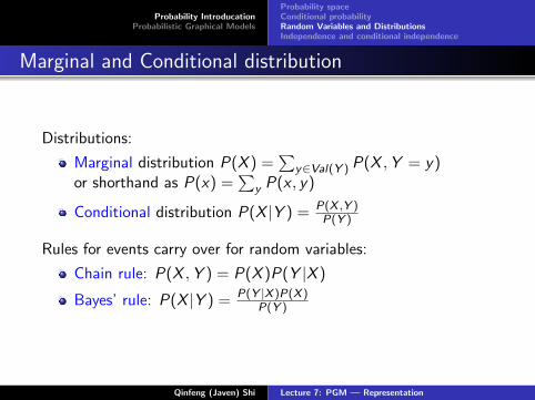
Marginal and Conditional distribution
Distributions:
Marginal distribution P(X ) =∑
y∈Val(Y ) P(X ,Y = y)or shorthand as P(x) =
∑y P(x , y)
Conditional distribution P(X |Y ) = P(X ,Y )P(Y )
Rules for events carry over for random variables:
Chain rule: P(X ,Y ) = P(X )P(Y |X )
Bayes’ rule: P(X |Y ) = P(Y |X )P(X )P(Y )
Qinfeng (Javen) Shi Lecture 7: PGM — Representation
Probability IntroducationProbabilistic Graphical Models
Probability spaceConditional probabilityRandom Variables and DistributionsIndependence and conditional independence
Independence and conditional independence
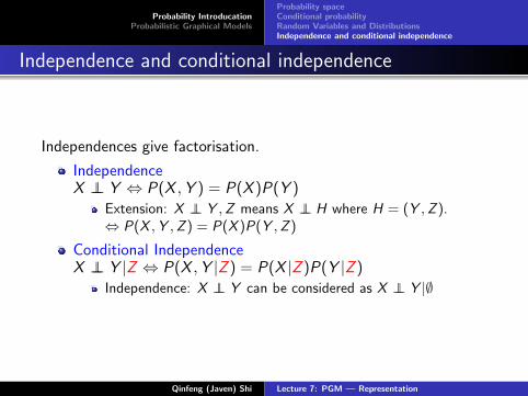
Independences give factorisation.
IndependenceX ⊥⊥ Y ⇔ P(X ,Y ) = P(X )P(Y )
Extension: X ⊥⊥ Y ,Z means X ⊥⊥ H where H = (Y ,Z ).⇔ P(X ,Y ,Z ) = P(X )P(Y ,Z )
Conditional IndependenceX ⊥⊥ Y |Z ⇔ P(X ,Y |Z ) = P(X |Z )P(Y |Z )
Independence: X ⊥⊥ Y can be considered as X ⊥⊥ Y |∅
Qinfeng (Javen) Shi Lecture 7: PGM — Representation
Probability IntroducationProbabilistic Graphical Models
Probability spaceConditional probabilityRandom Variables and DistributionsIndependence and conditional independence
Properties
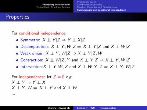
For conditional independence:
Symmetry: X ⊥⊥ Y |Z ⇒ Y ⊥⊥ X |ZDecomposition: X ⊥⊥ Y ,W |Z ⇒ X ⊥⊥ Y |Z and X ⊥⊥W |ZWeak union: X ⊥⊥ Y ,W |Z ⇒ X ⊥⊥ Y |Z ,WContraction: X ⊥⊥W |Z ,Y and X ⊥⊥ Y |Z ⇒ X ⊥⊥ Y ,W |ZIntersection:X ⊥⊥ Y |W ,Z and X ⊥⊥W |Y ,Z ⇒ X ⊥⊥ Y ,W |Z
For independence: let Z = ∅ e.g.X ⊥⊥ Y ⇒ Y ⊥⊥ XX ⊥⊥ Y ,W ⇒ X ⊥⊥ Y and X ⊥⊥W...
Qinfeng (Javen) Shi Lecture 7: PGM — Representation
Probability IntroducationProbabilistic Graphical Models
Probability spaceConditional probabilityRandom Variables and DistributionsIndependence and conditional independence
Marginal and MAP Queries
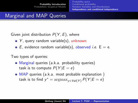
Given joint distribution P(Y ,E ), where
Y , query random variable(s), unknown
E , evidence random variable(s), observed i.e. E = e.
Two types of queries:
Marginal queries (a.k.a. probability queries)task is to compute P(Y |E = e)
MAP queries (a.k.a. most probable explanation )task is to find y∗ = argmaxy∈Val(Y ) P(Y |E = e)
Qinfeng (Javen) Shi Lecture 7: PGM — Representation

Probability IntroducationProbabilistic Graphical Models
Probability spaceConditional probabilityRandom Variables and DistributionsIndependence and conditional independence
Break
Take a break ...
Qinfeng (Javen) Shi Lecture 7: PGM — Representation
Probability IntroducationProbabilistic Graphical Models
History and booksRepresentationsFactorisationIndependences
Scenario 1
A
C
B
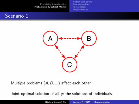
Multiple problems (A,B, ...) affect each other
Joint optimal solution of all 6= the solutions of individuals
Qinfeng (Javen) Shi Lecture 7: PGM — Representation
Probability IntroducationProbabilistic Graphical Models
History and booksRepresentationsFactorisationIndependences
Scenario 2
Two variables X ,Y each taking 10 possible values.Listing P(X ,Y ) for each possible value of X ,Y requiresspecifying/computing 102 many probabilities.
What if we have 1000 variables each taking 10 possible values?⇒ 101000 many probabilities
⇒ Difficult to store, and query naively.
Qinfeng (Javen) Shi Lecture 7: PGM — Representation
Probability IntroducationProbabilistic Graphical Models
History and booksRepresentationsFactorisationIndependences
Scenario 2
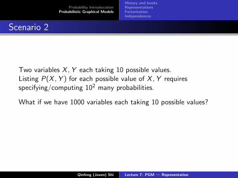
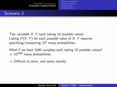
Two variables X ,Y each taking 10 possible values.Listing P(X ,Y ) for each possible value of X ,Y requiresspecifying/computing 102 many probabilities.
What if we have 1000 variables each taking 10 possible values?
⇒ 101000 many probabilities
⇒ Difficult to store, and query naively.
Qinfeng (Javen) Shi Lecture 7: PGM — Representation
Probability IntroducationProbabilistic Graphical Models
History and booksRepresentationsFactorisationIndependences
Scenario 2
Two variables X ,Y each taking 10 possible values.Listing P(X ,Y ) for each possible value of X ,Y requiresspecifying/computing 102 many probabilities.
What if we have 1000 variables each taking 10 possible values?⇒ 101000 many probabilities
⇒ Difficult to store, and query naively.
Qinfeng (Javen) Shi Lecture 7: PGM — Representation
Probability IntroducationProbabilistic Graphical Models
History and booksRepresentationsFactorisationIndependences
Remedy
Structured Learning, specially Probabilistic Graphical Models(PGMs).
Qinfeng (Javen) Shi Lecture 7: PGM — Representation
Probability IntroducationProbabilistic Graphical Models
History and booksRepresentationsFactorisationIndependences
PGMs
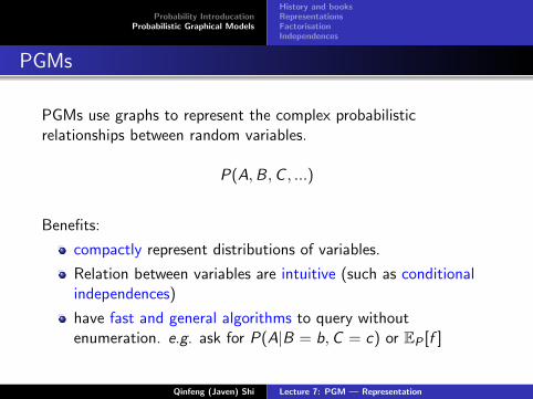
PGMs use graphs to represent the complex probabilisticrelationships between random variables.
P(A,B,C , ...)
Benefits:
compactly represent distributions of variables.
Relation between variables are intuitive (such as conditionalindependences)
have fast and general algorithms to query withoutenumeration. e.g. ask for P(A|B = b,C = c) or EP [f ]
Qinfeng (Javen) Shi Lecture 7: PGM — Representation

Probability IntroducationProbabilistic Graphical Models
History and booksRepresentationsFactorisationIndependences
An Example
G
I
J
S
D
H
L
Difficulty Intelligence
Grade
Happy
Letter
SAT
Job
Intuitive
Qinfeng (Javen) Shi Lecture 7: PGM — Representation
Probability IntroducationProbabilistic Graphical Models
History and booksRepresentationsFactorisationIndependences
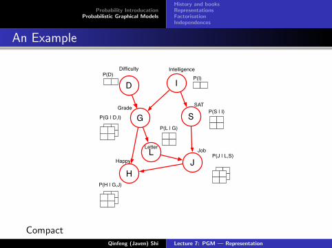
An Example
G
I
J
S
D
H
L
Difficulty Intelligence
Grade
Happy
Letter
SAT
Job
P(I)
P(S | I)
P(J | L,S)
P(D)
P(G | D,I)
P(H | G,J)
P(L | G)
CompactQinfeng (Javen) Shi Lecture 7: PGM — Representation
Probability IntroducationProbabilistic Graphical Models
History and booksRepresentationsFactorisationIndependences
History
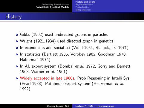
Gibbs (1902) used undirected graphs in particles
Wright (1921,1934) used directed graph in genetics
In economists and social sci (Wold 1954, Blalock, Jr. 1971)
In statistics (Bartlett 1935, Vorobev 1962, Goodman 1970,Haberman 1974)
In AI, expert system (Bombal et al. 1972, Gorry and Barnett1968, Warner et al. 1961)
Widely accepted in late 1980s. Prob Reasoning in Intelli Sys(Pearl 1988), Pathfinder expert system (Heckerman et al.1992)
Qinfeng (Javen) Shi Lecture 7: PGM — Representation
Probability IntroducationProbabilistic Graphical Models
History and booksRepresentationsFactorisationIndependences
History
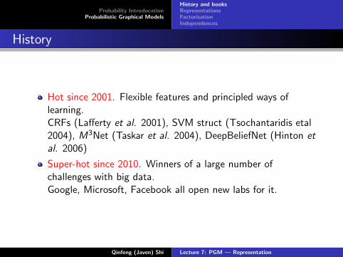
Hot since 2001. Flexible features and principled ways oflearning.CRFs (Lafferty et al. 2001), SVM struct (Tsochantaridis etal2004), M3Net (Taskar et al. 2004), DeepBeliefNet (Hinton etal. 2006)
Super-hot since 2010. Winners of a large number ofchallenges with big data.Google, Microsoft, Facebook all open new labs for it.
Qinfeng (Javen) Shi Lecture 7: PGM — Representation

Probability IntroducationProbabilistic Graphical Models
History and booksRepresentationsFactorisationIndependences
History
Qinfeng (Javen) Shi Lecture 7: PGM — Representation
Probability IntroducationProbabilistic Graphical Models
History and booksRepresentationsFactorisationIndependences
Good books
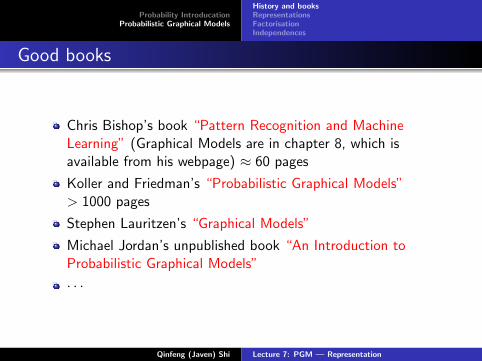
Chris Bishop’s book “Pattern Recognition and MachineLearning” (Graphical Models are in chapter 8, which isavailable from his webpage) ≈ 60 pages
Koller and Friedman’s “Probabilistic Graphical Models”> 1000 pages
Stephen Lauritzen’s “Graphical Models”
Michael Jordan’s unpublished book “An Introduction toProbabilistic Graphical Models”
· · ·
Qinfeng (Javen) Shi Lecture 7: PGM — Representation
Probability IntroducationProbabilistic Graphical Models
History and booksRepresentationsFactorisationIndependences
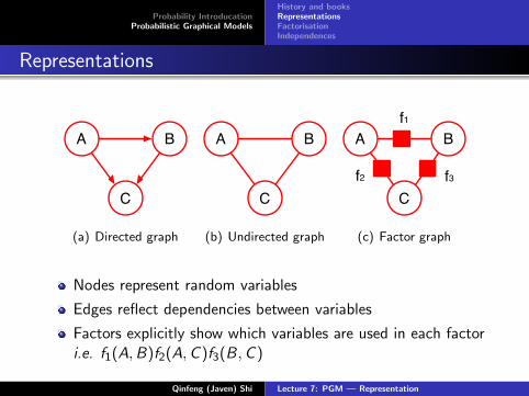
Representations
A
C
B
(a) Directed graph
A
C
B
(b) Undirected graph
A
C
B
f2
f1
f3
(c) Factor graph
Nodes represent random variables
Edges reflect dependencies between variables
Factors explicitly show which variables are used in each factori.e. f1(A,B)f2(A,C )f3(B,C )
Qinfeng (Javen) Shi Lecture 7: PGM — Representation
Probability IntroducationProbabilistic Graphical Models
History and booksRepresentationsFactorisationIndependences
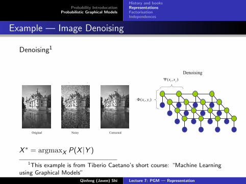
Example — Image Denoising
Denoising1
Applications in Vision and PR
Image denoising
Original CorrectedNoisy
Denoising
Real Applications
),( ii yxΦ
),( ji xxΨ
X ∗ = argmaxX P(X |Y )
1This example is from Tiberio Caetano’s short course: “Machine Learningusing Graphical Models”
Qinfeng (Javen) Shi Lecture 7: PGM — Representation
Probability IntroducationProbabilistic Graphical Models
History and booksRepresentationsFactorisationIndependences
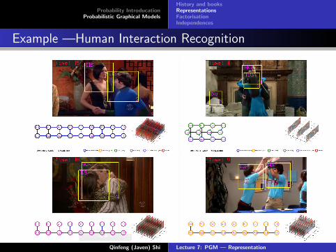
Example —Human Interaction Recognition
Qinfeng (Javen) Shi Lecture 7: PGM — Representation
Probability IntroducationProbabilistic Graphical Models
History and booksRepresentationsFactorisationIndependences
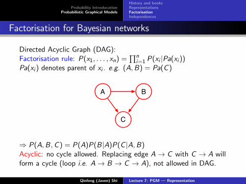
Factorisation for Bayesian networks
Directed Acyclic Graph (DAG):Factorisation rule: P(x1, . . . , xn) =
∏ni=1 P(xi |Pa(xi ))
Pa(xi ) denotes parent of xi . e.g. (A,B) = Pa(C )
A
C
B
⇒ P(A,B,C ) = P(A)P(B|A)P(C |A,B)Acyclic: no cycle allowed. Replacing edge A→ C with C → A willform a cycle (loop i.e. A→ B → C → A), not allowed in DAG.
Qinfeng (Javen) Shi Lecture 7: PGM — Representation
Probability IntroducationProbabilistic Graphical Models
History and booksRepresentationsFactorisationIndependences
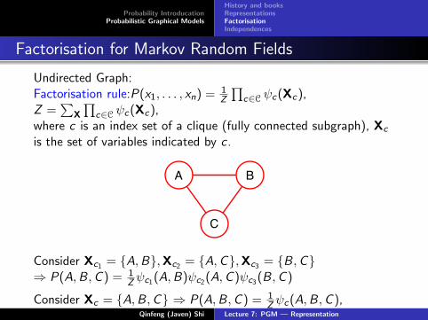
Factorisation for Markov Random Fields
Undirected Graph:Factorisation rule:P(x1, . . . , xn) = 1
Z
∏c∈C ψc(Xc),
Z =∑
X
∏c∈C ψc(Xc),
where c is an index set of a clique (fully connected subgraph), Xc
is the set of variables indicated by c.
A
C
B
Consider Xc1 = A,B,Xc2 = A,C,Xc3 = B,C⇒ P(A,B,C ) = 1
Z ψc1(A,B)ψc2(A,C )ψc3(B,C )
Consider Xc = A,B,C ⇒ P(A,B,C ) = 1Z ψc(A,B,C ),
Qinfeng (Javen) Shi Lecture 7: PGM — Representation
Probability IntroducationProbabilistic Graphical Models
History and booksRepresentationsFactorisationIndependences
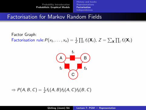
Factorisation for Markov Random Fields
Factor Graph:Factorisation rule:P(x1, . . . , xn) = 1
Z
∏i fi (Xi ), Z =
∑X
∏i fi (Xi )
A
C
B
f2
f1
f3
⇒ P(A,B,C ) = 1Z f1(A,B)f2(A,C )f3(B,C )
Qinfeng (Javen) Shi Lecture 7: PGM — Representation
Probability IntroducationProbabilistic Graphical Models
History and booksRepresentationsFactorisationIndependences
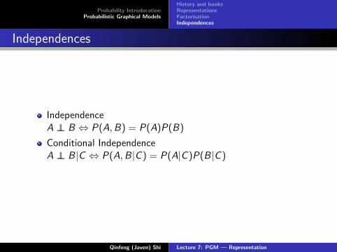
Independences
IndependenceA ⊥⊥ B ⇔ P(A,B) = P(A)P(B)
Conditional IndependenceA ⊥⊥ B|C ⇔ P(A,B|C ) = P(A|C )P(B|C )
Qinfeng (Javen) Shi Lecture 7: PGM — Representation
Probability IntroducationProbabilistic Graphical Models
History and booksRepresentationsFactorisationIndependences
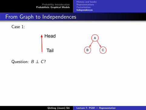
From Graph to Independences
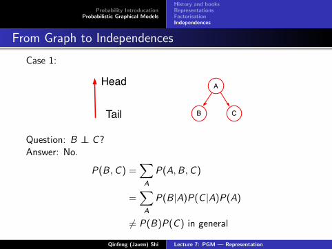
Case 1:
Head
Tail
A
CB
Question: B ⊥⊥ C?
Answer: No.
P(B,C ) =∑A
P(A,B,C )
=∑A
P(B|A)P(C |A)P(A)
6= P(B)P(C ) in general
Qinfeng (Javen) Shi Lecture 7: PGM — Representation
Probability IntroducationProbabilistic Graphical Models
History and booksRepresentationsFactorisationIndependences
From Graph to Independences
Case 1:
Head
Tail
A
CB
Question: B ⊥⊥ C?Answer: No.
P(B,C ) =∑A
P(A,B,C )
=∑A
P(B|A)P(C |A)P(A)
6= P(B)P(C ) in general
Qinfeng (Javen) Shi Lecture 7: PGM — Representation
Probability IntroducationProbabilistic Graphical Models
History and booksRepresentationsFactorisationIndependences
From Graph to Independences
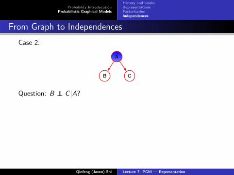
Case 2:
A
CB
Question: B ⊥⊥ C |A?
Answer: Yes.
P(B,C |A) =P(A,B,C )
P(A)
=P(B|A)P(C |A)P(A)
P(A)
= P(B|A)P(C |A)
Qinfeng (Javen) Shi Lecture 7: PGM — Representation
Probability IntroducationProbabilistic Graphical Models
History and booksRepresentationsFactorisationIndependences
From Graph to Independences
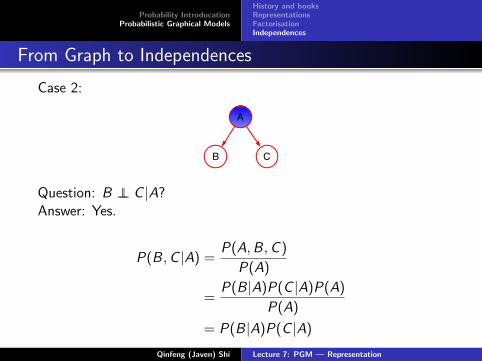
Case 2:
A
CB
Question: B ⊥⊥ C |A?Answer: Yes.
P(B,C |A) =P(A,B,C )
P(A)
=P(B|A)P(C |A)P(A)
P(A)
= P(B|A)P(C |A)
Qinfeng (Javen) Shi Lecture 7: PGM — Representation
Probability IntroducationProbabilistic Graphical Models
History and booksRepresentationsFactorisationIndependences
From graphs to independences
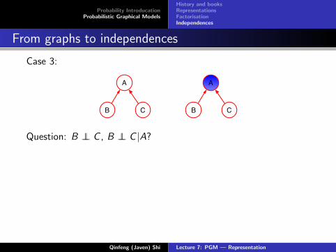
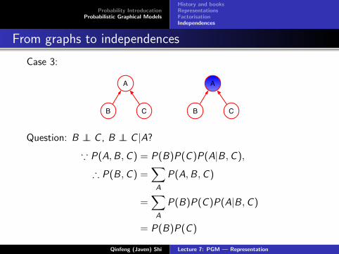
Case 3:
A
CB
A
CB
Question: B ⊥⊥ C , B ⊥⊥ C |A?
∵ P(A,B,C ) = P(B)P(C )P(A|B,C ),
∴ P(B,C ) =∑A
P(A,B,C )
=∑A
P(B)P(C )P(A|B,C )
= P(B)P(C )
Qinfeng (Javen) Shi Lecture 7: PGM — Representation
Probability IntroducationProbabilistic Graphical Models
History and booksRepresentationsFactorisationIndependences
From graphs to independences
Case 3:
A
CB
A
CB
Question: B ⊥⊥ C , B ⊥⊥ C |A?
∵ P(A,B,C ) = P(B)P(C )P(A|B,C ),
∴ P(B,C ) =∑A
P(A,B,C )
=∑A
P(B)P(C )P(A|B,C )
= P(B)P(C )
Qinfeng (Javen) Shi Lecture 7: PGM — Representation
Probability IntroducationProbabilistic Graphical Models
History and booksRepresentationsFactorisationIndependences
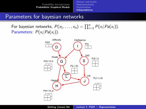
Parameters for bayesian networks
For bayesian networks, P(x1, . . . , xn) =∏n
i=1 P(xi |Pa(xi )).Parameters: P(xi |Pa(xi )).
G
I
J
S
D
H
L
Difficulty Intelligence
Grade
Happy
Letter
SAT
Job
P(I)
P(S | I)
P(J | L,S)
P(D)
P(G | D,I)
P(H | G,J)
P(L | G)
Qinfeng (Javen) Shi Lecture 7: PGM — Representation
Probability IntroducationProbabilistic Graphical Models
History and booksRepresentationsFactorisationIndependences
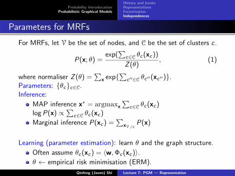
Parameters for MRFs
For MRFs, let V be the set of nodes, and C be the set of clusters c .
P(x; θ) =exp(
∑c∈C θc(xc))
Z (θ), (1)
where normaliser Z (θ) =∑
x exp∑
c ′′∈C θc ′′(xc ′′).Parameters: θcc∈C.Inference:
MAP inference x∗ = argmaxx∑
c∈C θc(xc)logP(x) ∝
∑c∈C θc(xc)
Marginal inference P(xc) =∑
xV /cP(x)
Learning (parameter estimation): learn θ and the graph structure.
Often assume θc(xc) = 〈w,Φc(xc)〉.θ ← empirical risk minimisation (ERM).
Qinfeng (Javen) Shi Lecture 7: PGM — Representation
Probability IntroducationProbabilistic Graphical Models
History and booksRepresentationsFactorisationIndependences
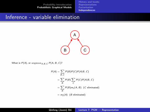
Inference - variable elimination
A
CB
What is P(A), or argmaxA,B,C P(A, B, C)?
P(A) =∑B,C
P(B)P(C)P(A|B, C)
=∑B
P(B)∑C
P(C)P(A|B, C)
=∑B
P(B)m1(A, B) (C eliminated)
= m2(A) (B eliminated)
Qinfeng (Javen) Shi Lecture 7: PGM — Representation
Probability IntroducationProbabilistic Graphical Models
History and booksRepresentationsFactorisationIndependences
Inference - variable elimination
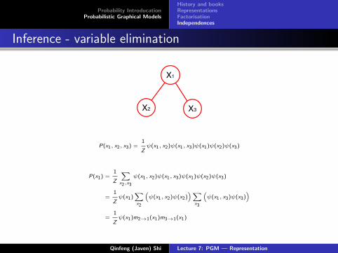
X3X2
X1
P(x1, x2, x3) =1
Zψ(x1, x2)ψ(x1, x3)ψ(x1)ψ(x2)ψ(x3)
P(x1) =1
Z
∑x2,x3
ψ(x1, x2)ψ(x1, x3)ψ(x1)ψ(x2)ψ(x3)
=1
Zψ(x1)
∑x2
(ψ(x1, x2)ψ(x2)
)∑x3
(ψ(x1, x3)ψ(x3)
)
=1
Zψ(x1)m2→1(x1)m3→1(x1)
Qinfeng (Javen) Shi Lecture 7: PGM — Representation
Probability IntroducationProbabilistic Graphical Models
History and booksRepresentationsFactorisationIndependences
Inference - variable elimination
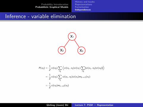
X3X2
X1
P(x2) =1
Zψ(x2)
∑x1
(ψ(x1, x2)ψ(x1)
∑x3
[ψ(x1, x3)ψ(x3)])
=1
Zψ(x2)
∑x1
ψ(x1, x2)ψ(x1)m3→1(x1)
=1
Zψ(x2)m1→2(x2)
Qinfeng (Javen) Shi Lecture 7: PGM — Representation
Probability IntroducationProbabilistic Graphical Models
History and booksRepresentationsFactorisationIndependences
Inference - Message Passing
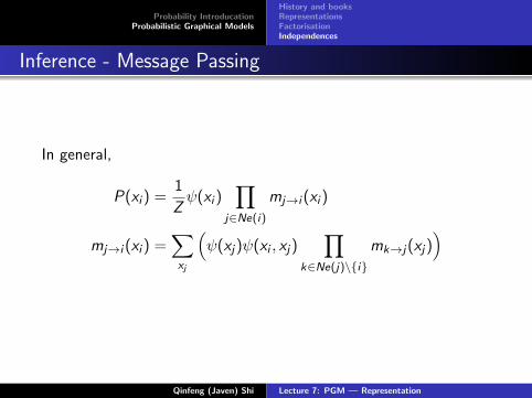
In general,
P(xi ) =1
Zψ(xi )
∏j∈Ne(i)
mj→i (xi )
mj→i (xi ) =∑xj
(ψ(xj)ψ(xi , xj)
∏k∈Ne(j)\i
mk→j(xj))
Qinfeng (Javen) Shi Lecture 7: PGM — Representation

Probability IntroducationProbabilistic Graphical Models
History and booksRepresentationsFactorisationIndependences
That’s all
Thanks!
Qinfeng (Javen) Shi Lecture 7: PGM — Representation