Lecture 7:Greedy Algorithms II

Shang-Hua Teng

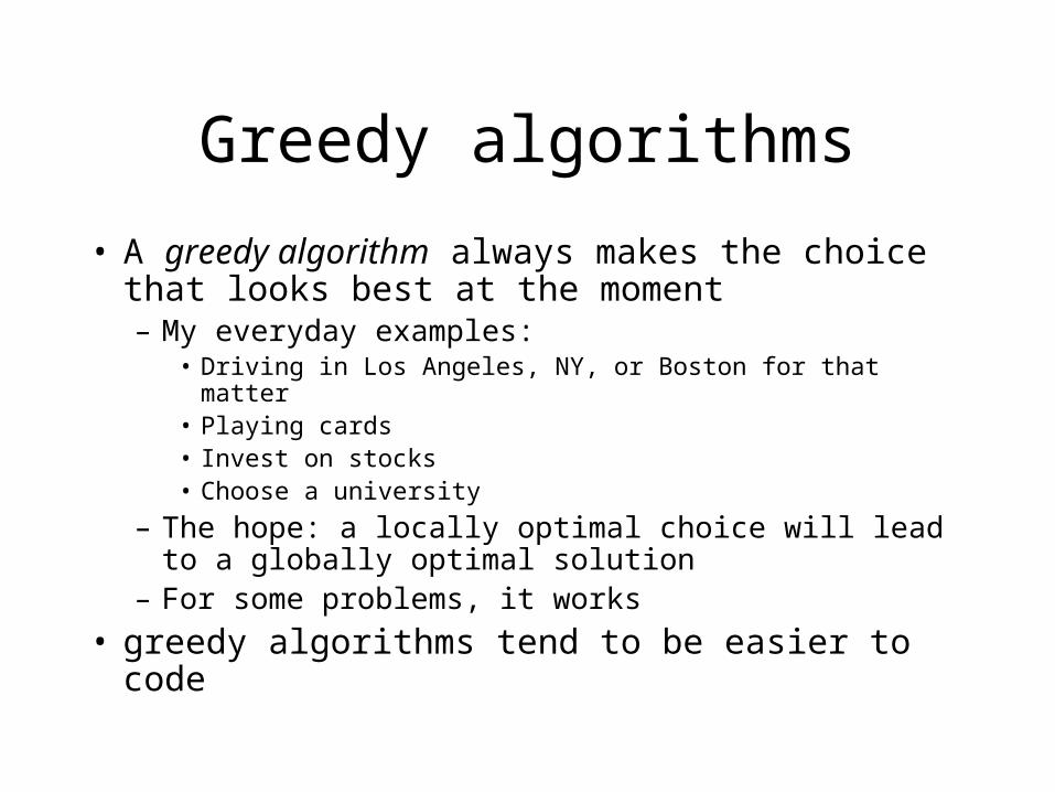
Greedy algorithms

• A greedy algorithm always makes the choice that looks best at the moment– My everyday examples:

• Driving in Los Angeles, NY, or Boston for that matter• Playing cards• Invest on stocks• Choose a university

– The hope: a locally optimal choice will lead to a globally optimal solution

– For some problems, it works

• greedy algorithms tend to be easier to code

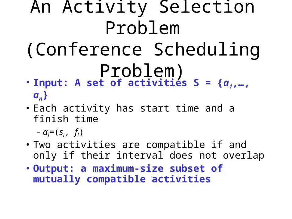
An Activity Selection Problem(Conference Scheduling Problem)

• Input: A set of activities S = {a1,…, an}• Each activity has start time and a finish time

– ai=(si, fi)

• Two activities are compatible if and only if their interval does not overlap

• Output: a maximum-size subset of mutually compatible activities

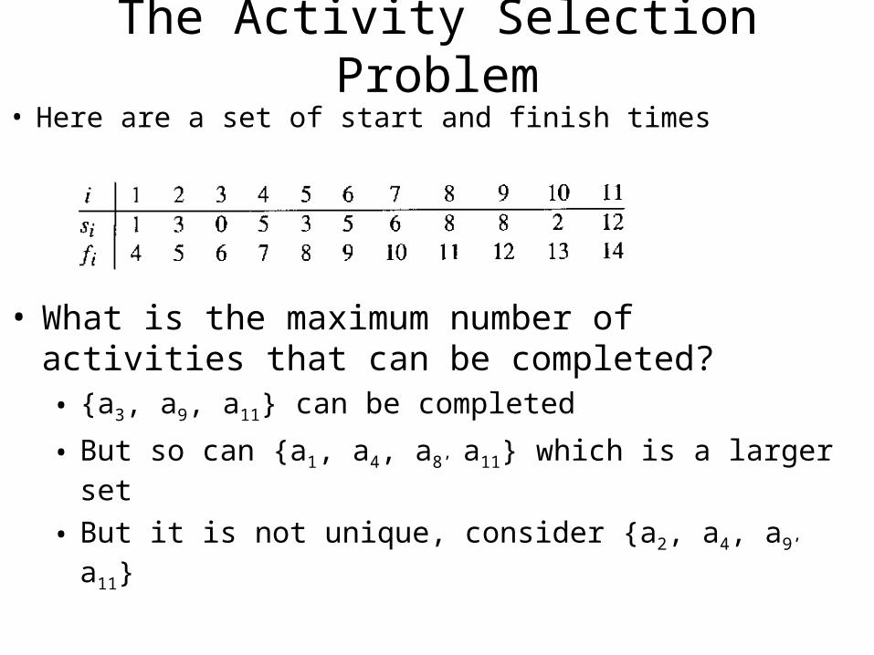
The Activity Selection Problem

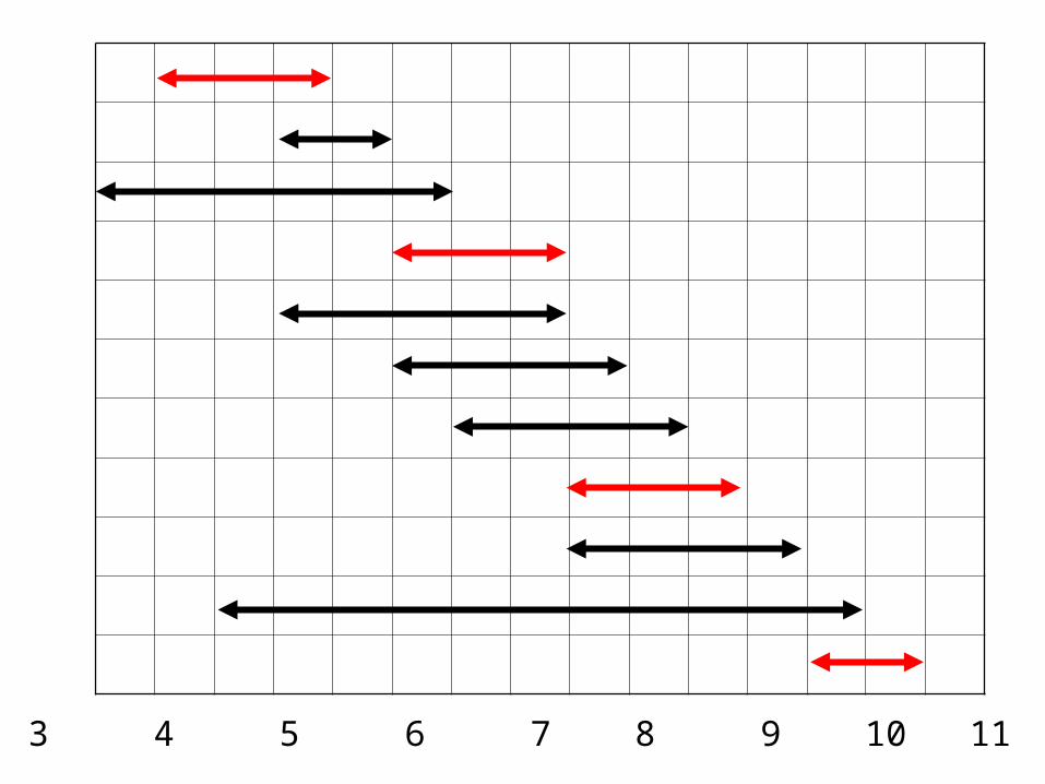
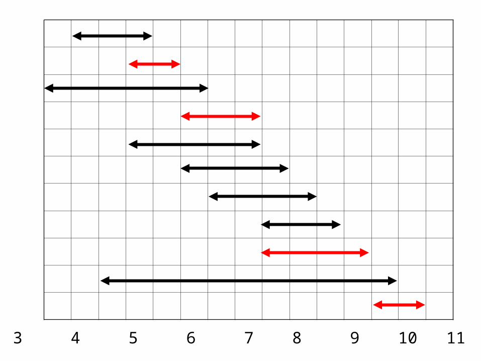
• Here are a set of start and finish times

• What is the maximum number of activities that can be completed?• {a3, a9, a11} can be completed

• But so can {a1, a4, a8’ a11} which is a larger set

• But it is not unique, consider {a2, a4, a9’ a11}

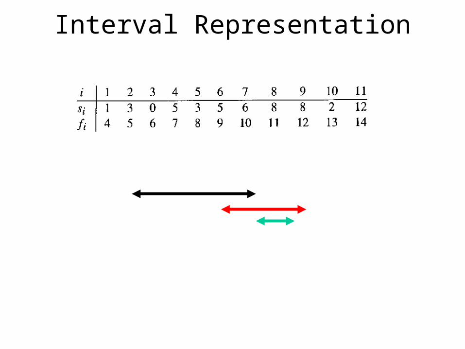
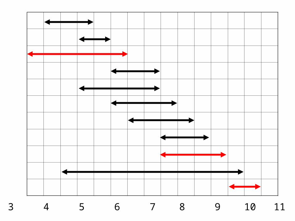
Interval Representation

0 1 2 3 4 5 6 7 8 9 10 11 12 13 14 15

0 1 2 3 4 5 6 7 8 9 10 11 12 13 14 15

0 1 2 3 4 5 6 7 8 9 10 11 12 13 14 15

0 1 2 3 4 5 6 7 8 9 10 11 12 13 14 15

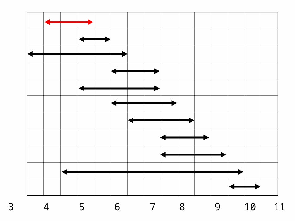
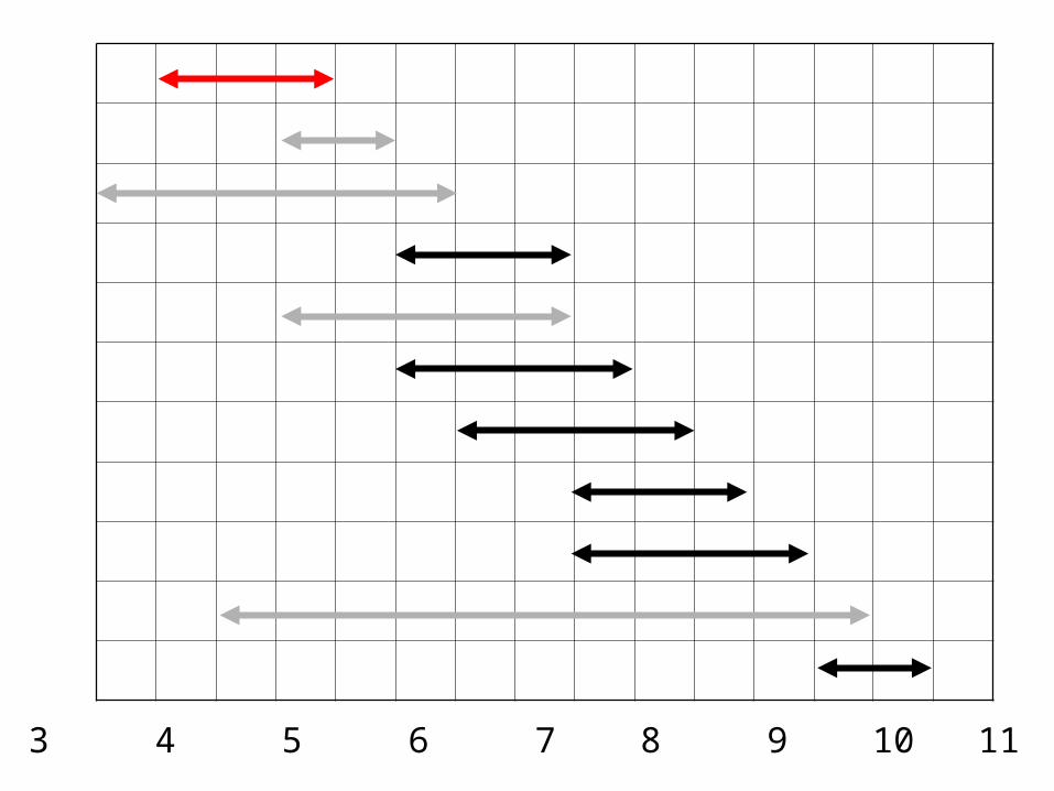
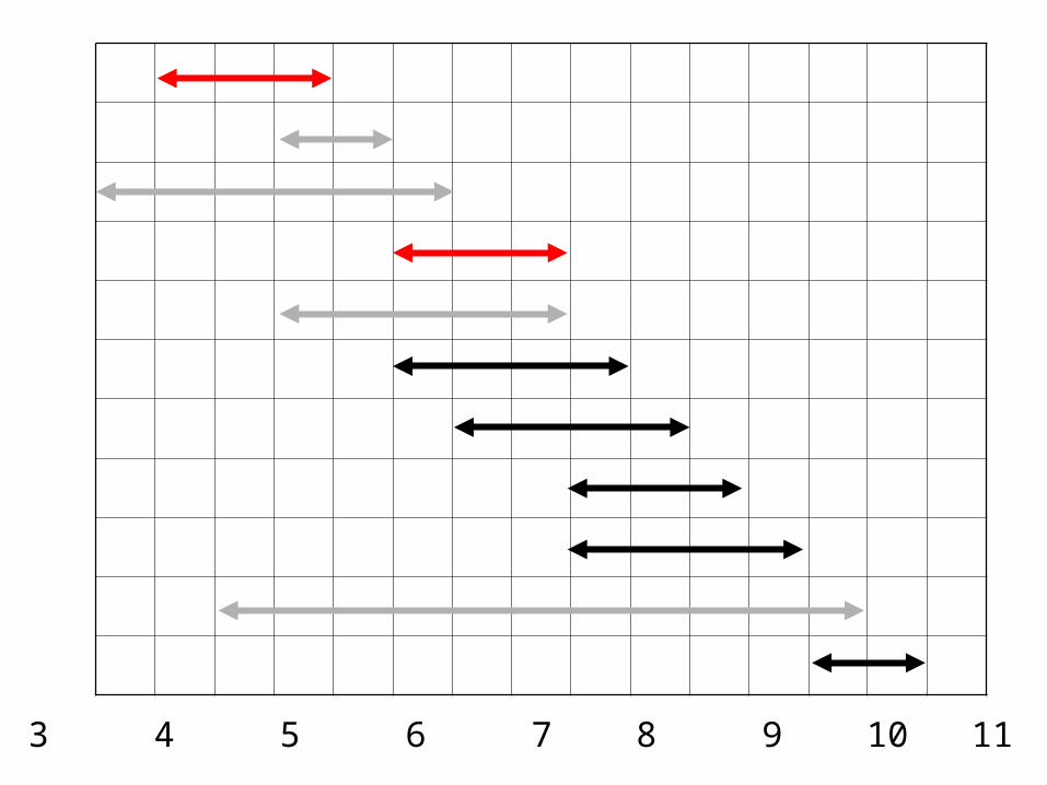
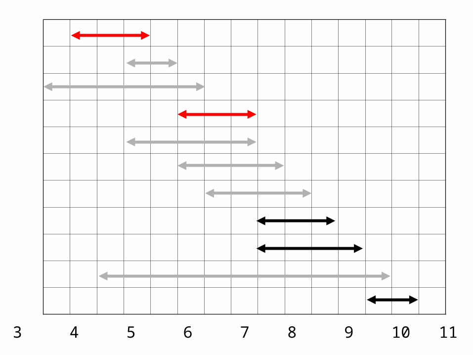
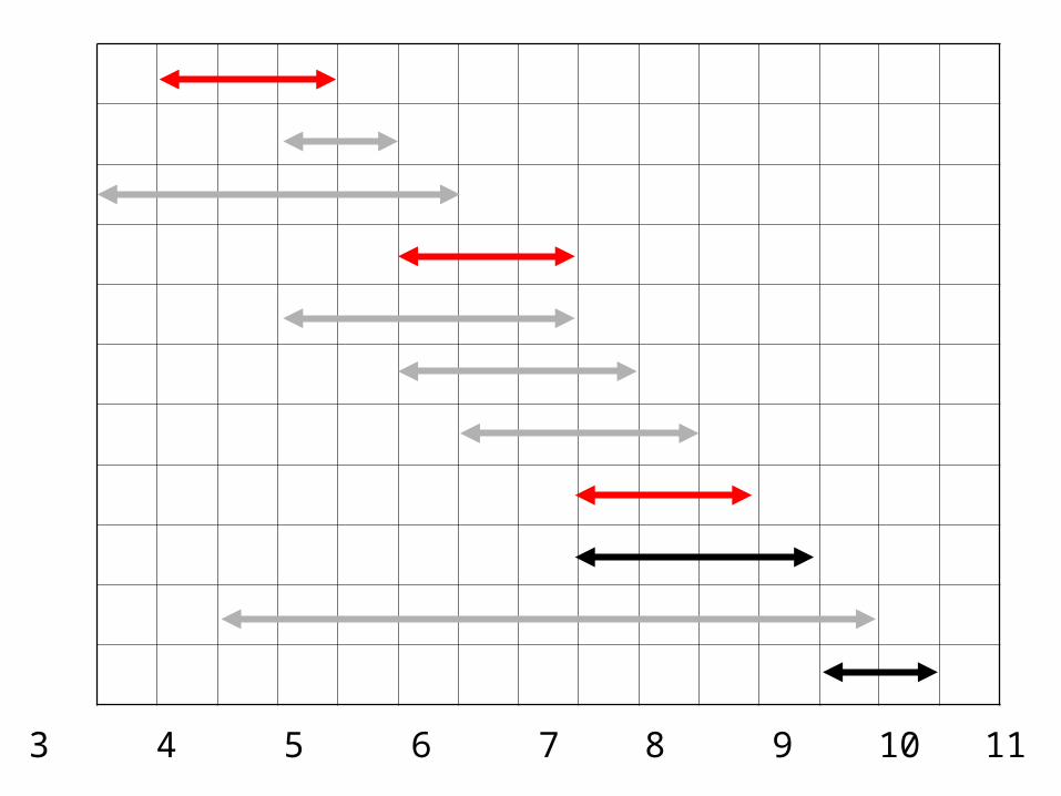
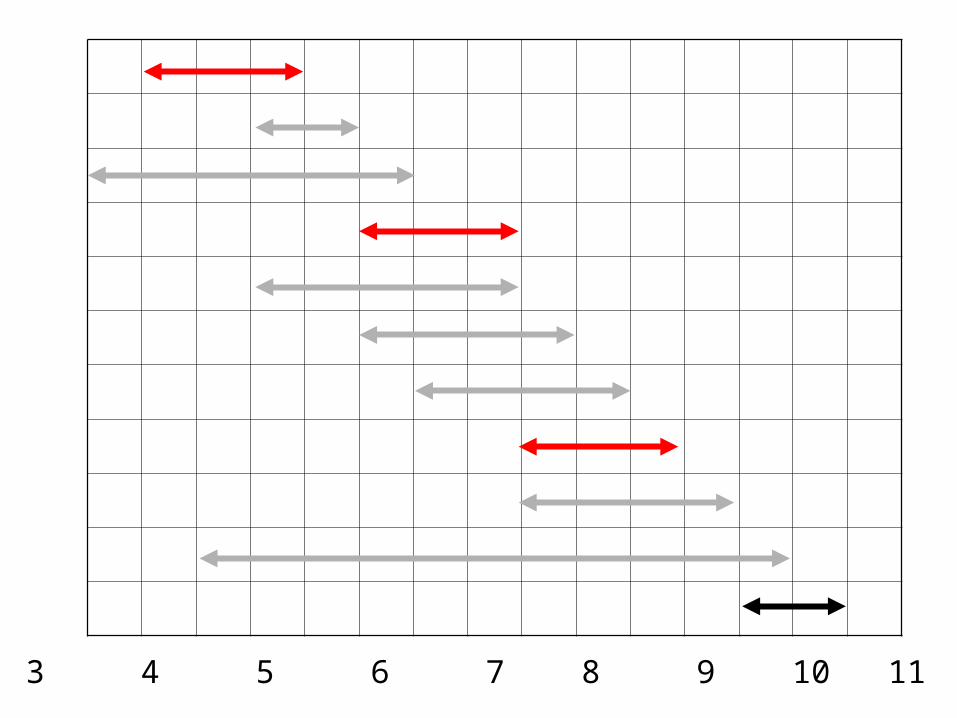
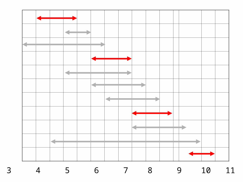
Early Finish Greedy

• Select the activity with the earliest finish

• Eliminate the activities that could not be scheduled

• Repeat!

0 1 2 3 4 5 6 7 8 9 10 11 12 13 14 15

0 1 2 3 4 5 6 7 8 9 10 11 12 13 14 15

0 1 2 3 4 5 6 7 8 9 10 11 12 13 14 15

0 1 2 3 4 5 6 7 8 9 10 11 12 13 14 15

0 1 2 3 4 5 6 7 8 9 10 11 12 13 14 15

0 1 2 3 4 5 6 7 8 9 10 11 12 13 14 15

0 1 2 3 4 5 6 7 8 9 10 11 12 13 14 15

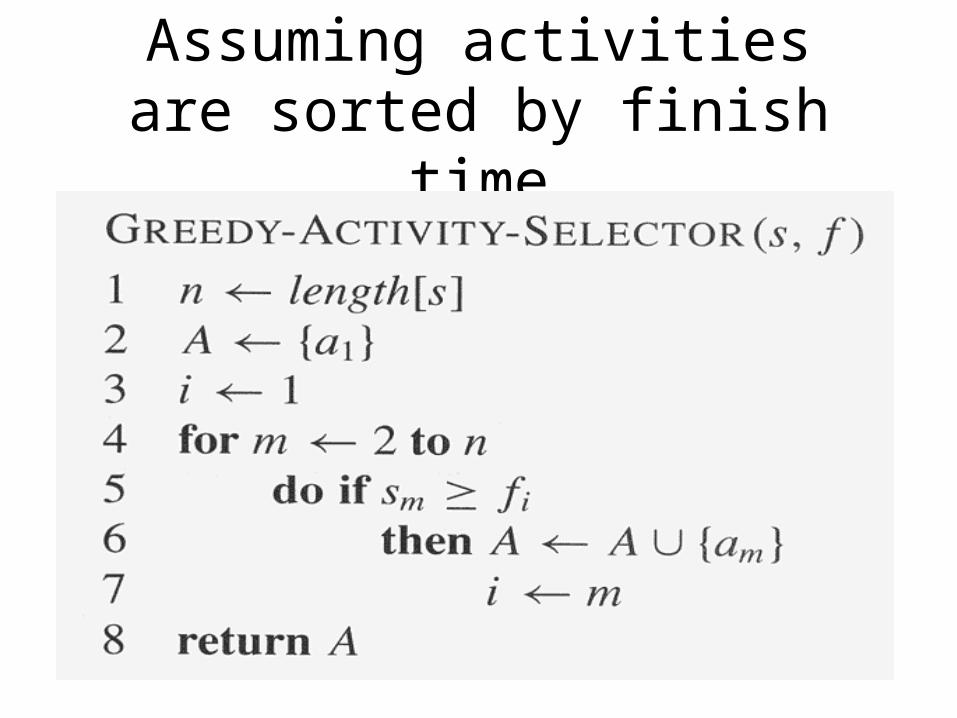
Assuming activities are sorted by finish time

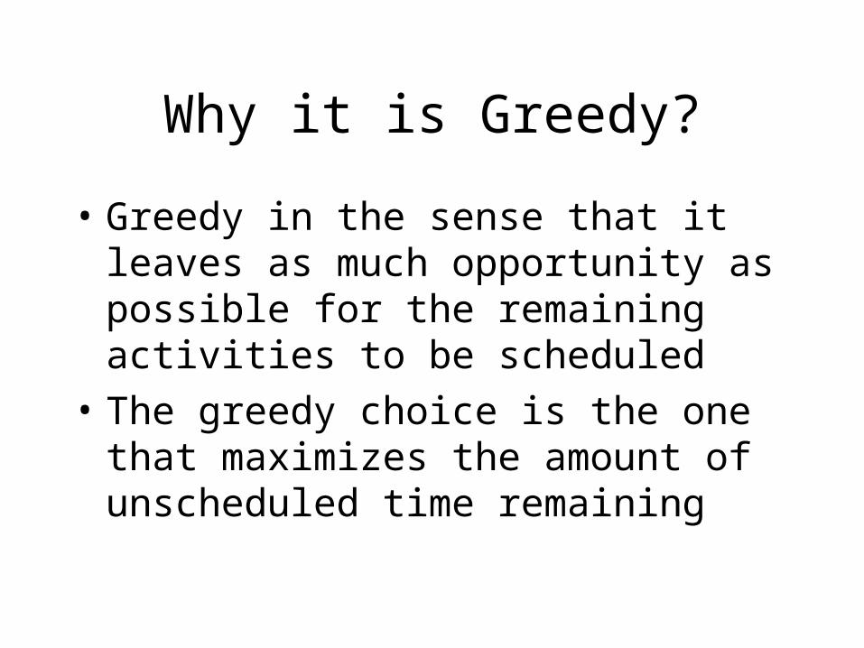
Why it is Greedy?

• Greedy in the sense that it leaves as much opportunity as possible for the remaining activities to be scheduled

• The greedy choice is the one that maximizes the amount of unscheduled time remaining

Why this Algorithm is Optimal?• We will show that this algorithm uses the

following properties

• The problem has the optimal substructure property

• The algorithm satisfies the greedy-choice property

• Thus, it is Optimal

Greedy-Choice Property• Show there is an optimal solution that begins with a greedy

choice (with activity 1, which as the earliest finish time)• Suppose A S in an optimal solution

– Order the activities in A by finish time. The first activity in A is k• If k = 1, the schedule A begins with a greedy choice

• If k 1, show that there is an optimal solution B to S that begins with the greedy choice, activity 1

– Let B = A – {k} {1}• f1 fk activities in B are disjoint (compatible)

• B has the same number of activities as A

• Thus, B is optimal

Optimal Substructures– Once the greedy choice of activity 1 is made, the problem

reduces to finding an optimal solution for the activity-selection problem over those activities in S that are compatible with activity 1

• Optimal Substructure

• If A is optimal to S, then A’ = A – {1} is optimal to S’={i S: si f1}

• Why?– If we could find a solution B’ to S’ with more activities than A’, adding

activity 1 to B’ would yield a solution B to S with more activities than A contradicting the optimality of A

– After each greedy choice is made, we are left with an optimization problem of the same form as the original problem

• By induction on the number of choices made, making the greedy choice at every step produces an optimal solution

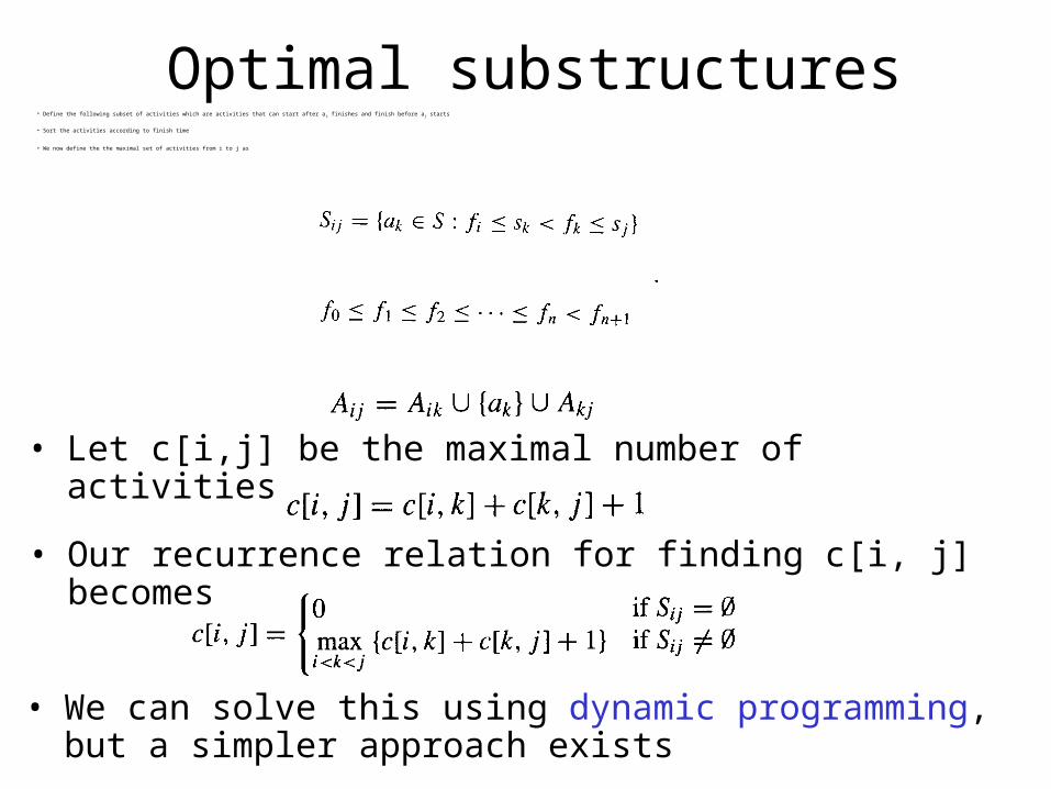
Optimal substructures• Define the following subset of activities which are activities that can start after ai finishes and finish before aj starts

• Sort the activities according to finish time

• We now define the the maximal set of activities from i to j as

• Let c[i,j] be the maximal number of activities

• We can solve this using dynamic programming, but a simpler approach exists

• Our recurrence relation for finding c[i, j] becomes

Elements of Greedy Strategy

• An greedy algorithm makes a sequence of choices, each of the choices that seems best at the moment is chosen– NOT always produce an optimal solution

• Two ingredients that are exhibited by most problems that lend themselves to a greedy strategy– Greedy-choice property

– Optimal substructure

Greedy-Choice Property• A globally optimal solution can be arrived at by

making a locally optimal (greedy) choice– Make whatever choice seems best at the moment and

then solve the sub-problem arising after the choice is made

– The choice made by a greedy algorithm may depend on choices so far, but it cannot depend on any future choices or on the solutions to sub-problems

• Usually progress in a top-down fashion making one greedy choice on after another, iteratively reducing each given problem instance to a smaller one

• Of course, we must prove that a greedy choice at each step yields a globally optimal solution

Optimal Substructures

• A problem exhibits optimal substructure if an optimal solution to the problem contains within it optimal solutions to sub-problems– If an optimal solution A to S begins with activity

1, then A’ = A – {1} is optimal to S’={i S: si f1}

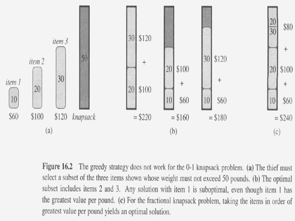
Knapsack Problem• You want to pack n items in your luggage

– The ith item is worth vi dollars and weighs wi pounds

– Take a valuable a load as possible, but cannot exceed W pounds

– vi , wi, W are integers

• 0-1 knapsack each item is taken or not taken• Fractional knapsack fractions of items can be taken• Both exhibit the optimal-substructure property

– 0-1: consider a optimal solution. If item j is removed from the load, the remaining load must be the most valuable load weighing at most W-wj

– Fractional: If w of item j is removed from the optimal load, the remaining load must be the most valuable load weighing at most W-w that can be taken from other n-1 items plus wj – w of item j

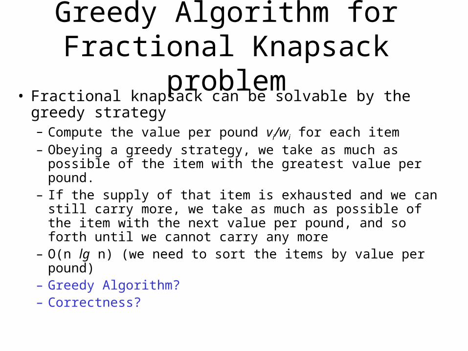
Greedy Algorithm for Fractional Knapsack problem

• Fractional knapsack can be solvable by the greedy strategy– Compute the value per pound vi/wi for each item– Obeying a greedy strategy, we take as much as possible of the

item with the greatest value per pound.– If the supply of that item is exhausted and we can still carry

more, we take as much as possible of the item with the next value per pound, and so forth until we cannot carry any more

– O(n lg n) (we need to sort the items by value per pound)– Greedy Algorithm? – Correctness?

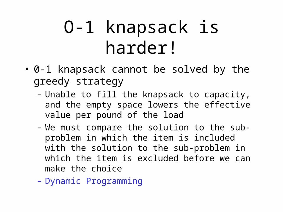
O-1 knapsack is harder!

• 0-1 knapsack cannot be solved by the greedy strategy– Unable to fill the knapsack to capacity, and the empty

space lowers the effective value per pound of the load

– We must compare the solution to the sub-problem in which the item is included with the solution to the sub-problem in which the item is excluded before we can make the choice

– Dynamic Programming

Next Week

• Ben Hescott will be guest lecturer and he will present dynamic programming

• I will be away for a conference

• Both Ben and TF will offer more office hour to cover me.

• TF: T 12:30 – 2:00 and TR: 9:30—11:00am