Lecture 6 Polar Codinghomepage.ntu.edu.tw/~ihwang/Teaching/Fa16/Slides/IT...IEEE TRANSACTIONS ON INFORMATION THEORY, VOL. 55, NO. 7, JULY 2009 3051 Channel Polarization: A Method for

Lecture 6Polar Coding

I-Hsiang Wang

Department of Electrical EngineeringNational Taiwan University

[email protected]

December 5, 2016

1 / 63 I-Hsiang Wang IT Lecture 6

mailto:[email protected]

In Pursuit of Shannon's Limit

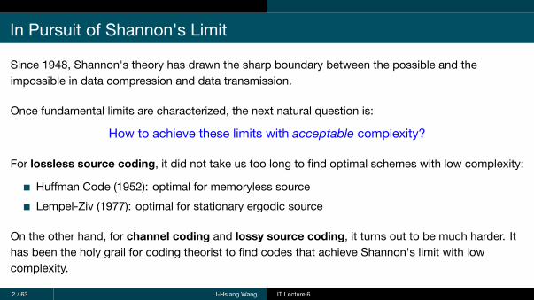
Since 1948, Shannon's theory has drawn the sharp boundary between the possible and theimpossible in data compression and data transmission.

Once fundamental limits are characterized, the next natural question is:

How to achieve these limits with acceptable complexity?

For lossless source coding, it did not take us too long to find optimal schemes with low complexity:

Huffman Code (1952): optimal for memoryless sourceLempel-Ziv (1977): optimal for stationary ergodic source

On the other hand, for channel coding and lossy source coding, it turns out to be much harder. Ithas been the holy grail for coding theorist to find codes that achieve Shannon's limit with lowcomplexity.


In Pursuit of Capacity-Achieving Codes

Two barriers in pursuing low-complexity capacity-achieving codes:1 Lack of explicit construction. In Shannon's proof, it is only proved that there exists coding

schemes that achieve capacity.2 Lack of structure to reduce complexity. In the proof of coding theorems, complexity issues

are often neglected, while codes with structures are hard to prove to achieve capacity.Since 90's, several practical codes were found to approach capacity – turbo code, low-densityparity-check (LDPC) code, etc. They perform well empirically, but lack rigorous proof of optimality.

The first provably capacity-achieving coding scheme with acceptable complexity is polar code,introduced by Erdal Arıkan in 2007.

Later in 2012, spatially coupled LDPC codes were also shown to achieve capacity (ShrinivasKudekar, Tom Richardson, and Rüediger Urbanke).


IEEE TRANSACTIONS ON INFORMATION THEORY, VOL. 55, NO. 7, JULY 2009 3051

Channel Polarization: A Method for ConstructingCapacity-Achieving Codes for Symmetric

Binary-Input Memoryless ChannelsErdal Arıkan, Senior Member, IEEE

Abstract—A method is proposed, called channel polarization,to construct code sequences that achieve the symmetric capacity

of any given binary-input discrete memoryless channel(B-DMC) . The symmetric capacity is the highest rate achiev-able subject to using the input letters of the channel with equalprobability. Channel polarization refers to the fact that it is pos-sible to synthesize, out of independent copies of a given B-DMC

, a second set of binary-input channelssuch that, as becomes large, the fraction of indices for which

is near approaches and the fraction for whichis near approaches . The polarized channelsare well-conditioned for channel coding: one need only

send data at rate through those with capacity near and at ratethrough the remaining. Codes constructed on the basis of this ideaare called polar codes. The paper proves that, given any B-DMC

with and any target rate , there exists asequence of polar codes such that has block-length

, rate , and probability of block error under suc-cessive cancellation decoding bounded asindependently of the code rate. This performance is achievable byencoders and decoders with complexity for each.

Index Terms—Capacity-achieving codes, channel capacity,channel polarization, Plotkin construction, polar codes, Reed–Muller (RM) codes, successive cancellation decoding.

I. INTRODUCTION AND OVERVIEW

A FASCINATING aspect of Shannon’s proof of the noisychannel coding theorem is the random-coding method

that he used to show the existence of capacity-achieving codesequences without exhibiting any specific such sequence [1].Explicit construction of provably capacity-achieving codesequences with low encoding and decoding complexities hassince then been an elusive goal. This paper is an attempt tomeet this goal for the class of binary-input discrete memorylesschannels (B-DMCs).

We will give a description of the main ideas and results of thepaper in this section. First, we give some definitions and statesome basic facts that are used throughout the paper.

Manuscript received October 14, 2007; revised August 13, 2008. Current ver-sion published June 24, 2009. This work was supported in part by The Scien-tific and Technological Research Council of Turkey (TÜBITAK) under Project107E216 and in part by the European Commission FP7 Network of ExcellenceNEWCOM++ under Contract 216715. The material in this paper was presentedin part at the IEEE International Symposium on Information Theory (ISIT),Toronto, ON, Canada, July 2008.

The author is with the Department of Electrical-Electronics Engineering,Bilkent University, Ankara, 06800, Turkey (e-mail: [email protected]).

Communicated by Y. Steinberg, Associate Editor for Shannon Theory.Color versions of Figures 4 and 7 in this paper are available online at http://

ieeexplore.ieee.org.Digital Object Identifier 10.1109/TIT.2009.2021379

A. Preliminaries

We write to denote a generic B-DMC withinput alphabet , output alphabet , and transition probabilities

. The input alphabet will always be, the output alphabet and the transition probabilities may

be arbitrary. We write to denote the channel correspondingto uses of ; thus, with

.Given a B-DMC , there are two channel parameters of pri-

mary interest in this paper: the symmetric capacity

and the Bhattacharyya parameter

These parameters are used as measures of rate and reliability,respectively. is the highest rate at which reliable commu-nication is possible across using the inputs of with equalfrequency. is an upper bound on the probability of max-imum-likelihood (ML) decision error when is used only onceto transmit a or .

It is easy to see that takes values in . Throughout,we will use base- logarithms; hence, will also takevalues in . The unit for code rates and channel capacitieswill be bits.

Intuitively, one would expect that iff ,and iff . The following bounds, proved inthe Appendix, make this precise.

Proposition 1: For any B-DMC , we have

(1)

(2)

The symmetric capacity equals the Shannon capacitywhen is a symmetric channel, i.e., a channel for which thereexists a permutation of the output alphabet such that i)

and ii) for all . The bi-nary symmetric channel (BSC) and the binary erasure channel(BEC) are examples of symmetric channels. A BSC is a B-DMC

with and. A B-DMC is called a BEC if for each , either

or . In the latter case,

0018-9448/$25.00 © 2009 IEEE

The paper wins the 2010 Information Theory Society Best Paper Award.


Overview

When Arıkan introduced polar codes in 2007, he focus on achieving capacity for the generalbinary-input memoryless symmetric channels (BMSC), including BSC, BEC, etc.

Later, polar codes are shown to be optimal in many other settings, including lossy source coding,non-binary-input channels, multiple access channels, channel coding with encoder side information(Gelfand-Pinsker), source coding with side information (Wyner-Ziv), etc.

Instead of giving a comprehensive introduction, we shall focus on polar coding for channel coding.The outline is as follows:

1 First we introduce the concept of channel polarization.

2 Second we explore polar coding for binary input channels.

3 Finally we briefly talk about polar coding for source coding (source polarization).


Notations

In channel coding, we use the DMC N times where N is the blocklength of the coding scheme.

Since the channel is the main focus, we use the following notations throughout this lecture:

W to denote the channel PY |X

P to denote the input distribution PX

I (P,W ) to denote I (X ;Y ).

Since we focus on BMSC, and X ∼ Ber(12

)achieves the channel capacity of any BMSC, we shall

use I (W ) (slight abuse of notation) to denote I (P,W ) when the input P is Ber(12

).

In other words, the channel capacity of a BMSCW is I (W ).


Polarization

1 PolarizationBasic Channel TransformationChannel Polarization

2 Polar CodingEncoding and Decoding ArchitecturesPerformance Analysis


Polarization

Single Usage of ChannelW

X YW

N Usage of ChannelW

...

ENC DEC

W

W

W

M M

X1

X2

XN

Y1

Y2

YN


Polarization

Arıkan's Idea

...

Pre-Processing

W

W

W

X1

X2

XN

Y1

Y2

YNUN

U2

U1

Post-Processing

V1

V2

VN

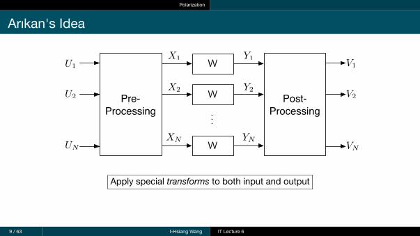
Apply special transforms to both input and output


Polarization

Arıkan's Idea

W1

...

W2

WNUN

U2

U1 V1

V2

VN


Polarization

Arıkan's Idea

W1

...

W2

WNUN

U2

U1 V1

V2

VN

Roughly N I (W ) channels with capacity � 1


Polarization

Arıkan's Idea

W1

...

W2

WNUN

U2

U1 V1

V2

VN

Roughly N I (W ) channels with capacity � 1

Roughly N (1 � I (W )) channels with capacity � 0

Equivalently some perfect channels and some useless channels −→ Polarization

Coding becomes extremely simple: simply use those perfect channels for uncoded transmission,and throw those useless channels away.


Polarization Basic Channel Transformation





Arıkan's Basic Channel Transformation

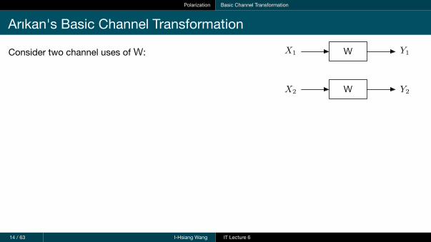
Consider two channel uses ofW:


X1

X2

W

W

Y1

Y2


Arıkan's Basic Channel Transformation

Consider two channel uses ofW:

Apply the pre-processor: X1 = U1 ⊕ U2, X2 = U2,where U1 ⊥⊥ U2, U1, U2 ∼ Ber

(12

).

We now have two synthetic channels induced by the above procedure:

W− : U1 → V1 ≜ (Y1, Y2)

W+ : U2 → V2 ≜ (Y1, Y2, U1)

The above transform yields the following two crucial phenomenon:

I (W− ) ≤ I (W ) ≤ I (W+ ) (Polarization)

I (W− ) + I (W+ ) = 2I (W ) (Conservation of Information)


W

W

Y1

Y2U2

U1


Example: Binary Erasure Channel

Example 1

LetW be a BEC with erasure probability ε ∈ (0, 1), and I (W ) = 1− ε. Find the values of I (W− )and I (W+ ), and verify the above properties.

sol: IntuitivelyW− is worse thanW andW+ is better thanW:

ForW−, input is U1, output is (Y1, Y2): Only when both Y1 and Y2 are not erased, one can figure outU1! =⇒ W− is BEC with erasure probability 1− (1− ε)

2= 2ε− ε2.

ForW+, input is U2, output is (Y1, Y2, U1): As long as one of Y1 and Y2 are not erased, one can figureout U2! =⇒ W+ is BEC with erasure probability ε2.

Hence, I (W− ) = 1− 2ε+ ε2 and I (W+ ) = 1− ε2.



Example: Binary Symmetric Channel

Example 2

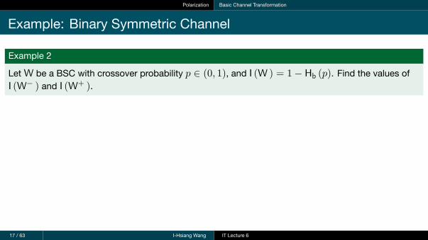
LetW be a BSC with crossover probability p ∈ (0, 1), and I (W ) = 1− Hb (p). Find the values ofI (W− ) and I (W+ ).



Basic Properties

Theorem 1For any BMSCW and the induced channels {W−,W+} from Arıkan's basic transformation, we have

I (W− ) ≤ I (W ) ≤ I (W+ ) with equality iff I (W ) = 0 or 1.

I (W− ) + I (W+ ) = 2I (W )

pf: We prove the conservation of information first:

I(W− )

+ I(W+

)= I (U1 ;Y1, Y2 ) + I (U2 ;Y1, Y2, U1 ) = I (U1 ;Y1, Y2 ) + I (U2 ;Y1, Y2 |U1 )

= I (U1, U2 ;Y1, Y2 ) = I (X1, X2 ;Y1, Y2 ) = I (X1 ;Y1 ) + I (X2 ;Y2 ) = 2I (W ) .

I (W+ ) = I (X2 ;Y1, Y2, U1 ) ≥ I (X2 ;Y2 ) = I (W ), and hence the first property holds.(Proof of the condition for equality is left as exercise.)



Extremal Channels

12.1. The Basic Channel Transformation 281

The clue is now to realize that we have equality in (12.27) if, and onlyif, Y1 is conditionally independent of X1 given U1 and Y2. This can happenonly in exactly two cases: Either W is useless, i.e., Y1 is independent of X1

and any other quantity related with X1 such that all conditioning disappearsand we have H(Y1)�H(Y1) in (12.25) (this corresponds to the situation whenI(W) = 0). Or W is perfect so that from Y2 we can perfectly recover U2 and— with the additional help of U1 — also X1 (this corresponds to the situationwhen I(W) = 1 bit).

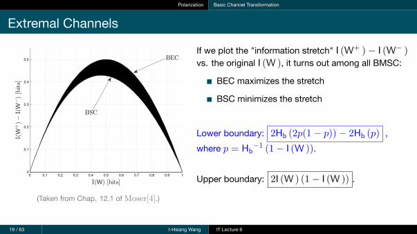
It can be shown that a BEC yields the largest di↵erence between I(W+)and I(W�) and the BSC yields the smallest di↵erence. Any other DMC willyield something in between. See Figure 12.4 for the corresponding plot.

0 0.1 0.2 0.3 0.4 0.5 0.6 0.7 0.8 0.9 10

0.1

0.2

0.3

0.4

0.5

I(W

+)−I(W

−

)[bits]

I(W) [bits]

BEC

BSC

Figure 12.4: Di↵erence of I(W+) and I(W�) as a function of I(W). We see thatunless the channel is extreme already, the di↵erence is strictlypositive. Moreover, the largest di↵erence is achieved for a BEC,while the BSC yields the smallest di↵erence.

Exercise 12.6. In this exercise you are asked to recreate the boundary curvesin Figure 12.4.

1. Start with W being a BEC with erasure probability �. Recall that I(W) =1� � bits, and then show that I(W+)� I(W�) = 2�(1� �) bits.

2. For W being a BSC with crossover probability ✏, recall that I(W) =1�Hb(✏) bits. Then, defining Z1 and Z2 being independent binary RVs

c� Copyright Stefan M. Moser, version 4.4, 31 Aug. 2015

(Taken from Chap. 12.1 of Moser[4].)

If we plot the "information stretch" I (W+ )− I (W− )vs. the original I (W ), it turns out among all BMSC:

BEC maximizes the stretch

BSC minimizes the stretch

Lower boundary: 2Hb (2p(1− p))− 2Hb (p) ,where p = Hb−1 (1− I (W )).

Upper boundary: 2I (W ) (1− I (W )) .


Polarization Channel Polarization





Recursive Application of Arıkan's Transformation

DuplicateW, apply the transformation, and getW− andW+.


W

W




DuplicateW− (andW+).


W

W

W

W





Apply the transformation onW−, and getW−− andW−+.


W

W

W

W






Apply the transformation onW+, and getW+− andW++.


W

W

W

W






Apply the transformation onW+, and getW+− andW++.

...

We can keep going and going, until the desired blocklengthis reached.


W

W

W

W

W

W

W

W


Polarized Channels after Recursive Application

After one recursion and gettingW− andW+, let us duplicate them.


W

W

W

W

Y1

Y2

Y3

Y4



Apply the transformation onW−:

W−− : U1 → ((Y1, Y2) , (Y3, Y4)) = Y 4

W−+ : U2 → ((Y1, Y2) , (Y3, Y4) , U1) =(Y 4, U1

)27 / 63 I-Hsiang Wang IT Lecture 6

W

W

W

W

U1

U2

Y1

Y2

Y3

Y4



Apply the transformation onW+:

W+− : U3 → ((Y1, Y2, U1 ⊕ U2) , (Y3, Y4, U2)) =(Y 4, U2

)W++ : U4 → ((Y1, Y2, U1 ⊕ U2) , (Y3, Y4, U2) , U3) =

(Y 4, U3


W

W

W

W

U3

U4

Y1

Y2

Y3

Y4

U1 � U2

U2



Putting things together, we have:

W−− : U1 →(Y 4, ∅

)W−+ : U2 →

(Y 4, U1

)W+− : U3 →

(Y 4, U2

)W++ : U4 →

(Y 4, U3


W

W

W

W

U1

U3

U2

U4

Y1

Y2

Y3

Y4




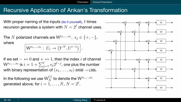
With proper naming of the inputs (do it yourself), ℓ-timesrecursion generates a system with N = 2ℓ channel uses.

The N polarized channels areWs1,...,sℓ , sj ∈ {+,−},where

Ws1,...,sℓ : Ui →(Y N , U i−1

).

If we set − ↔ 0 and + ↔ 1, then the index i of channelWs1,...,sℓ is i = 1 +

∑ℓj=1 sj2

ℓ−j , one plus the numberwith binary representation of (s1, . . . , sℓ) (MSB → LSB).

In the following we useW(i)N to denote theWs1,...,sℓ

generated above, for i = 1, . . . , N , N = 2ℓ.

W

W

W

W

W

W

W

W


Channel Polarization

Theorem 2 (Channel Polarization)

For any BMSCW, the polarized channels{W(i)

N

∣∣∣ i = 1, . . . , N}

(N = 2ℓ) satisfy the following:

For all a, b such that 0 < a < b < 1,

limN→∞

1N

∣∣∣{i : I(W(i)N

)∈ [0, a)

}∣∣∣ = 1− I (W ) and

limN→∞

1N

∣∣∣{i : I(W(i)N

)∈ (b, 1]

}∣∣∣ = I (W )

limN→∞

1N

∣∣∣{i : I(W(i)N

)∈ [a, b]

}∣∣∣ = 0

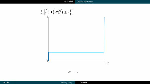
Interpretation: When N is sufficiently large, roughly N I (W ) of them are noiseless (capacity = 1),and N (1− I (W )) of them are useless (capacity = 0).



0 10

1

1N

!!!"i : I

#W(i)

N

$≤ ε

%!!!

�

N = 20



0 10

1

1N

!!!"i : I

#W(i)

N

$≤ ε

%!!!

�

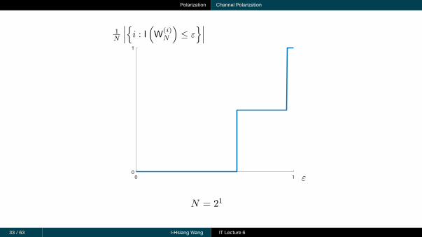
N = 21



0 10

1

1N

!!!"i : I

#W(i)

N

$≤ ε

%!!!

�

N = 22



0 10

1

1N

!!!"i : I

#W(i)

N

$≤ ε

%!!!

�

N = 24



0 10

1

1N

!!!"i : I

#W(i)

N

$≤ ε

%!!!

�

N = 28



0 10

1

1N

!!!"i : I

#W(i)

N

$≤ ε

%!!!

�

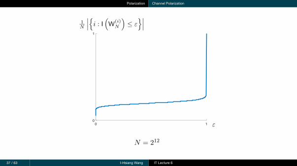
N = 212



0 10

1

1N

!!!"i : I

#W(i)

N

$≤ ε

%!!!

�

N = 220



0 10

1

1N

!!!"i : I

#W(i)

N

$≤ ε

%!!!

�

N = ∞



Proof of Channel Polarization

pf: Define the averaged first and second moment of{W(i)

2ℓ

∣∣∣ i = 1, . . . , 2ℓ}as follows: (2ℓ = N )

µℓ ≜ 12ℓ

∑2ℓ

i=1 I(W(i)

2ℓ

), νℓ ≜ 1

2ℓ

∑2ℓ

i=1

(I(W(i)

2ℓ

))2

Due to the conservation of information of Arıkan's transformaion (Theorem 1), µℓ = I (W ) for all ℓ.

As for the averaged second moment, note that

12

((I (W+ ))

2+ (I (W− ))

2)=

(12 (I (W+ ) + I (W− ))

)2+

(12 (I (W+ )− I (W− ))

)2= I (W )2 +

(12 (I (W+ )− I (W− ))

)2= I (W )2 +∆(W)2 ,

where ∆(W) ≜ 12 (I (W+ )− I (W− )).



νℓ+1 =12ℓ

2ℓ∑i=1

I(W(i)

2ℓ

)2+∆

(W(i)

2ℓ

)2

≥ νℓ + κ (a, b)2 θℓ (a, b) , (1)

where

κ(a, b) ≜ min {∆(WBSCa) ,∆(WBSCb) , }

θℓ(a, b) ≜ 12ℓ

∣∣∣{i : I(W(i)

2ℓ

)∈ [a, b]

}∣∣∣ .Hence, {νℓ} form a non-decreasing sequence.

Meanwhile, since all channels are binary-input,I(W(i)

2ℓ

)≤ 1, and therefore νℓ ≤ 1.

12.1. The Basic Channel Transformation 281

The clue is now to realize that we have equality in (12.27) if, and onlyif, Y1 is conditionally independent of X1 given U1 and Y2. This can happenonly in exactly two cases: Either W is useless, i.e., Y1 is independent of X1

and any other quantity related with X1 such that all conditioning disappearsand we have H(Y1)�H(Y1) in (12.25) (this corresponds to the situation whenI(W) = 0). Or W is perfect so that from Y2 we can perfectly recover U2 and— with the additional help of U1 — also X1 (this corresponds to the situationwhen I(W) = 1 bit).

It can be shown that a BEC yields the largest di↵erence between I(W+)and I(W�) and the BSC yields the smallest di↵erence. Any other DMC willyield something in between. See Figure 12.4 for the corresponding plot.

0 0.1 0.2 0.3 0.4 0.5 0.6 0.7 0.8 0.9 10

0.1

0.2

0.3

0.4

0.5

I(W

+)−I(W

−

)[bits]

I(W) [bits]

BEC

BSC

Figure 12.4: Di↵erence of I(W+) and I(W�) as a function of I(W). We see thatunless the channel is extreme already, the di↵erence is strictlypositive. Moreover, the largest di↵erence is achieved for a BEC,while the BSC yields the smallest di↵erence.

Exercise 12.6. In this exercise you are asked to recreate the boundary curvesin Figure 12.4.

1. Start with W being a BEC with erasure probability �. Recall that I(W) =1� � bits, and then show that I(W+)� I(W�) = 2�(1� �) bits.

2. For W being a BSC with crossover probability ✏, recall that I(W) =1�Hb(✏) bits. Then, defining Z1 and Z2 being independent binary RVs

c� Copyright Stefan M. Moser, version 4.4, 31 Aug. 2015

(Modified from Chap. 12.1 of Moser[4].)



Hence, ν0 ≤ ν1 ≤ . . . ≤ νℓ ≤ . . . ≤ 1 =⇒ limℓ→∞ νℓ exists.

By (1), we have

θℓ(a, b) ≤νℓ+1 − νℓκ(a, b)2

=⇒ limℓ→∞

θℓ(a, b) = 0. (since limℓ→∞ νℓ exists.)

Finally, define αℓ(a) ≜ 12ℓ

∣∣∣{i : I(W(i)

2ℓ

)∈ [0, a)

}∣∣∣ and βℓ(b) ≜ 12ℓ

∣∣∣{i : I(W(i)

2ℓ

)∈ (b, 1]

}∣∣∣.Observe that

I (W ) = µℓ ≤ a · αℓ(a) + b · θℓ(a, b) + 1 · βℓ(b) = a+ (b− a)θℓ(a, b) + (1− a)βℓ(b)

1− I (W ) = 1− µℓ ≤ 1− 0 · αℓ(a)− a · θℓ(a, b)− b · βℓ(b) = (1− b) + (b− a)θℓ(a, b) + bαℓ(a)

It is then not hard to show that lim infℓ→∞ βℓ(b) ≥ I (W ) and lim infℓ→∞ αℓ(b) ≥ 1− I (W ).

Proof is complete by sandwich principle.



From Channel Polarization to Polar CodingRecall the original goal:

...

Pre-Processing

W

W

W

X1

X2

XN

Y1

Y2

YNUN

U2

U1

Post-Processing

V1

V2

VN

Caveat:What we have done, however, it thefollowing: we created N = 2ℓ

polarized channels

W(i)N : Ui → Vi =

(Y N , U i−1

).

However, we cannot obtain the trueU i−1 from the channel output Y N .

This issue can be fixed by successive decoding, where Vi ≜ (Y N , U i−1) instead of (Y N , U i−1).

Encoding is based on those "synthetic" polarized channels {W(i)N }, and the i-th synthetic channel is

a good approximation as long as U i−1 = U i−1 with high probability.


Polar Coding




Polar Coding Encoding and Decoding Architectures





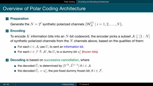
Overview of Polar Coding Architecture

1 PreparationGenerate the N = 2ℓ synthetic polarized channels {W(i)

N | i = 1, 2, . . . , N}.

2 EncodingTo encode K information bits into an N -bit codeword, the encoder picks a subset A ⊆ [1 : N ]of synthetic polarized channels from the N channels above, based on the qualities of them:

For each i ∈ A, use Ui to sent an information bit.For each i ∈ F ≜ Ac, fix Ui to a dummy bit u∗

i (frozen bits).

3 Decoding is based on successive cancellation, wherethe decoded Ui is determined by (Y N , U i−1) if i ∈ A.the decoded Ui = u∗

i , the pre-fixed dummy frozen bit, if i ∈ F .



Synthetic Polarized ChannelsFor the i-th synthesized channel, its input is Ui, output is

(Y N , U i−1

), and the

channel law is

W(i)N

(yN , ui−1

∣∣ui

)= 1

2N−1

1∑ui+1=0

...1∑

uN=0P(yN

∣∣uN),

where P(yN

∣∣uN)=

∏Ni=1W (yi|xi). The relationship between xN and uN is

described in the next slide.

Recursive Relation of Channel Laws

W(2k−1)2N

(y2N , u2k−2

∣∣u2k−1

)=

∑u2k=0,1

12W(k)

N

(y1:N , u2k−2

odd ⊕ u2k−2even

∣∣u2k−1 ⊕ u2k

)W(k)

N

(yN+1:2N , u2k−2

even∣∣u2k

)W(2k)

2N

(y2N , u2k−1

∣∣u2k

)= 1

2W(k)

N

(y1:N , u2k−2

odd ⊕ u2k−2even

∣∣u2k−1 ⊕ u2k

)W(k)

N

(yN+1:2N , u2k−2

even∣∣u2k

)



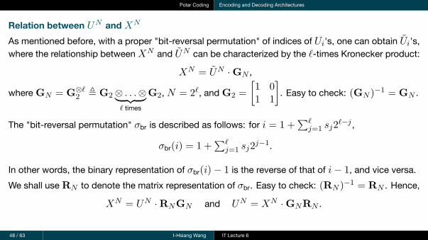
Relation between UN and XN

As mentioned before, with a proper "bit-reversal permutation" of indices of Ui's, one can obtain Ui's,where the relationship betweenXN and UN can be characterized by the ℓ-times Kronecker product:

XN = UN · GN ,

where GN = G⊗ℓ2 ≜ G2⊗ . . .⊗︸︷︷︸

ℓ times

G2, N = 2ℓ, and G2 =

[1 01 1

]. Easy to check: (GN )−1 = GN .

The "bit-reversal permutation" σbr is described as follows: for i = 1 +∑ℓ

j=1 sj2ℓ−j ,

σbr(i) = 1 +∑ℓ

j=1 sj2j−1.

In other words, the binary representation of σbr(i)− 1 is the reverse of that of i− 1, and vice versa.We shall use RN to denote the matrix representation of σbr. Easy to check: (RN )−1 = RN . Hence,

XN = UN · RNGN and UN = XN · GNRN .



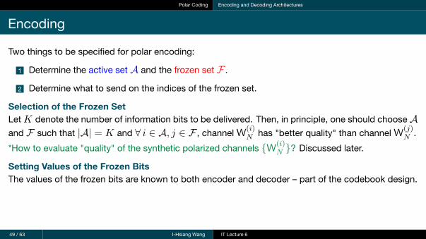
Encoding

Two things to be specified for polar encoding:

1 Determine the active set A and the frozen set F .

2 Determine what to send on the indices of the frozen set.

Selection of the Frozen SetLetK denote the number of information bits to be delivered. Then, in principle, one should chooseAand F such that |A| = K and ∀ i ∈ A, j ∈ F , channelW(i)

N has "better quality" than channelW(j)N .

*How to evaluate "quality" of the synthetic polarized channels {W(i)N }? Discussed later.

Setting Values of the Frozen BitsThe values of the frozen bits are known to both encoder and decoder – part of the codebook design.



Encoding Architecture

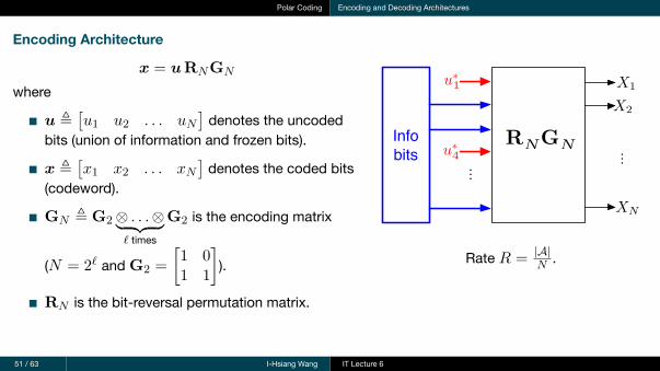
x = uRNGN

where

u ≜[u1 u2 . . . uN

]denotes the uncoded

bits (union of information and frozen bits).

x ≜[x1 x2 . . . xN

]denotes the coded bits

(codeword).

GN ≜ G2⊗ . . .⊗︸︷︷︸ℓ times

G2 is the encoding matrix

(N = 2ℓ and G2 =

[1 01 1

]).

RN is the bit-reversal permutation matrix.

X1

X2

XNUN

U2

U1

Rate R = |A|N .



Encoding Architecture

x = uRNGN

where

u ≜[u1 u2 . . . uN

]denotes the uncoded

bits (union of information and frozen bits).

x ≜[x1 x2 . . . xN

]denotes the coded bits

(codeword).

GN ≜ G2⊗ . . .⊗︸︷︷︸ℓ times

G2 is the encoding matrix

(N = 2ℓ and G2 =

[1 01 1

]).

RN is the bit-reversal permutation matrix.

X1

X2

XN

Info bits

Rate R = |A|N .



Decoding

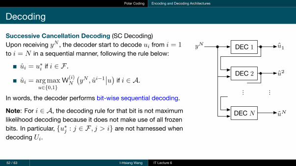
Successive Cancellation Decoding (SC Decoding)Upon receiving yN , the decoder start to decode ui from i = 1to i = N in a sequential manner, following the rule below:

ui = u∗i if i ∈ F .

ui = arg maxu∈{0,1}

W(i)N

(yN , ui−1

∣∣u) if i ∈ A.

In words, the decoder performs bit-wise sequential decoding.

Note: For i ∈ A, the decoding rule for that bit is not maximumlikelihood decoding because it does not make use of all frozenbits. In particular, {u∗j : j ∈ F , j > i} are not harnessed whendecoding Ui.

DEC

DEC

DEC


Polar Coding Performance Analysis





Probability of Error

Under SC decoding, probability of error of the proposed polar coding scheme depends on(1) channelW, (2) blocklength N , (3) code rate K

N , (4) frozen set F ⊂ [1 : N ], (5) frozen bits uF .Notation: here we use uF and uA to denote the frozen bits and information bits respectively.

First, define the average (over all codewords) probability of error with given frozen bits uF :

P(N)e

(KN ,F ,uF

)≜ P

{UN = UN

}=

∑uA∈{0,1}K

2−K · P{∃ i ∈ A s.t. Ui = Ui

∣∣∣UA = uA

}.

Next, we further average over uniformly randomly chosen frozen bits uF and define

P(N)e

(KN ,F

)≜

∑uF∈{0,1}N−K

2−(N−K) · P(N)e

(KN ,F ,uF

).



Upper Bounding the Probability of Error of Polar Coding (1)

Observe that P(N)e

(KN ,F

)= P

{∪i∈A{Ui = Ui, U

i−1 = U i−1}}

≤∑

i∈A P{Ui(Y

N , U i−1) = Ui, Ui−1 = U i−1

}, (2)

where Uii.i.d.∼ Ber

(12

), for all i = 1, 2, . . . , N . The inequality is due to union bound.

Recall that decoding function Ui(YN , U i−1) = arg max

u∈{0,1}W(i)

N

(Y N , U i−1

∣∣∣u). Hence,P{Ui(Y

N , U i−1) = Ui, Ui−1 = U i−1

}= P

{Ui(Y

N , U i−1) = Ui, Ui−1 = U i−1

}≤ P

{Ui(Y

N , U i−1) = Ui

}. (3)



Now things boil down to upper bounding P{Ui(Y

N , U i−1) = Ui

}, where

Ui(yN , ui−1) = arg max

u∈{0,1}W(i)

N

(yN , ui−1

∣∣u) . (4)

Key Observation: P{Ui(Y

N , U i−1) = Ui

}is the optimal error probability of error of a binary

detection problem, since the bitwise decoder (4) above is the corresponding MAP/ML detection rule!

Ui W(i)N

�Y N , U i�1

�MAP( ML)∼ Ber

!12

"

Next, we introduce Z (W) as an error probability upper bound for a binary detection problem withinput X ∼ Ber

(12

)and observation Y , following the probability transition lawW(y|x). Naturally it

measures the reliability of a channelW.



Bit-wise Decoding Error Probability

Lemma 1For a binary detection problem with input X ∼ Ber

(12

)and observation Y following the probability

transition lawW(y|x), the optimal probability of error (note: ML is optimal)

P{XML (Y ) = X

}≤ Z (W) , where Z (W) ≜

∑y∈Y

√W(y|0) ·W(y|1). (5)

pf: Recall that the ML detection rule: XML (y) = x ifW(y|x) ≥W(y|x⊕ 1). Hence,

P{XML (Y ) = X

}= EX,Y [1 {W(Y |X) <W(Y |X ⊕ 1)}] ≤ EX,Y

[√W(Y |X⊕1)W(Y |X)

].

It is not hard to verify that Z (W) = EX,Y

[√W(Y |X⊕1)W(Y |X)

](left as exercise).



Properties of the Reliability Function Z (·)

Proofs of the following properties are neglected here.1 Range of Z: 0 ≤ Z (W) ≤ 1. (By Cauchy-Schwarz)2 Polarization: under Arıkan's transformation,

Z (W+) = (Z (W))2, Z (W−) ≤ 2Z (W)− (Z (W))

2

Z (W+) + Z (W−) ≤ 2Z (W). (Reliability is improved after the polarization)Z (W+) ≤ Z (W) ≤ Z (W−).

3 Relation with I (W ): 1− Z(W) ≤ I (W ) ≤ 1− (Z(W))2.I (W ) ≈ 1 ⇐⇒ Z(W) ≈ 0

I (W ) ≈ 0 ⇐⇒ Z(W) ≈ 1

Hence, one can expect that channel polarization (Theorem 2) still holds if we change themeasure of "goodness" from capacity to reliability function.



Upper Bounding the Probability of Error of Polar Coding (2)

Combining (2), (3), and Lemma 1, we arrive at a nice upper bound on P(N)e

(KN ,F

):

P(N)e

(KN ,F

)≤

∑i∈A Z

(W(i)

N

). (6)

♢

Implications of Upper Bound (6):

1 How to choose the frozen set F? If we would like to minimize (6), we should choose A and Fsuch that Z

(W(i)

N

)≤ Z

(W(j)

N

)for all i ∈ A and j ∈ F . In other words, we use Z (·) to

evaluate the quality of the synthetic polarized channels.2 Suppose we can compute the asymptotic limit of the proportion of synthetic polarized channels

whose Z (·) is smaller than some δN = o(N−1

). If R is less than this limit, for sufficiently large

N , we can further upper bound (6) by NR · δN which will vanish as N → ∞.



Speed of Channel Polarization

In other words, we would like to have some theorem which gives us the following result:

limN→∞

1N

∣∣∣{i : Z (W(i)

N

)< δN

}∣∣∣ = I (W ).

This is a stronger version of channel polarization than Theorem 2.

To see this, note that we can easily replace I(W(i)

N

)by 1− Z

(W(i)

N

)in Theorem 2 and the results

remain to hold for constants a and b, where a, b = Θ(1), invariant to N .

However, the desired theorem requires replacing a and b by δN and 1− δN respectively, whereδN = o

(N−1

). The proof of Theorem 2 presented before cannot be extended to this case.



Nevertheless, Arıkan and Telatar proved an even stronger result, where δN = 2−Nβ , β ∈(0, 12

).

Below we present this result without proving it.

Theorem 3 (Rate of Channel Polarization [Arıkan-Telatar ISIT09])

Direct Part: For β ∈(0, 12

),

limN→∞

1

N

∣∣∣{i : Z (W(i)

N

)< 2−Nβ

}∣∣∣ = I (W ) (7)

limN→∞

1

N

∣∣∣{i : Z (W(i)

N

)> 1− 2−Nβ

}∣∣∣ = 1− I (W ) (8)

Converse Part: For β > 12 , if I (W ) < 1,

limN→∞

1

N

∣∣∣{i : Z (W(i)

N

)< 2−Nβ

}∣∣∣ = 0.



Coding Theorem for Polar Coding

Theorem 4 (Polar Coding Achieves Capacity of BMSC)

Suppose the frozen set F is chosen such that Z(W(i)

N

)≤ Z

(W(j)

N

)for all i ∈ A and j ∈ F . Then,

limN→∞

P(N)e (R,F) · 2Nβ

= 0 (9)

for any rate R < I (W ) and β ∈(0, 12

). In other words, P(N)

e (R,F) = o(2−Nβ

).

Note: (9) guarantees that the probability of error vanishes as N → ∞ for some choice of frozen bitsuF , as long as R < I (W ), the channel capacity. Hence, it shows that polar code can achieve thecapacity of the channelW.

Remark: In fact, for symmetric channels, it can be shown that (9) remains true even if we replaceP(N)e (R,F) by P(N)

e (R,F ,uF ) for any uF ∈ {0, 1}N(1−R). This will be explored in HW4.



pf: Fix some β′ ∈(β, 12

). Since R < I (W ), by Lemma 3, for N sufficiently large,∣∣∣{i : Z (

W(i)N

)< 2−Nβ′

}∣∣∣ > NR.

Since we pick A and F such that |A| = NR and all synthetic polarized channels with indices in Ahave smaller Z (·) than those in F , we have

Z(W(i)

N

)< 2−Nβ′

, ∀ i ∈ A.

Hence, by the upper bound (6), we conclude that

P(N)e (R,F) < NR · 2−Nβ′ =⇒ P(N)

e (R,F) · 2Nβ< NR · 2−(Nβ′−Nβ).

Proof is complete by observing limN→∞

NR · 2−(Nβ′−Nβ) = 0.


Documents

Lecture 6 Polar Codinghomepage.ntu.edu.tw/~ihwang/Teaching/Fa16/Slides/IT...IEEE TRANSACTIONS ON INFORMATION THEORY, VOL. 55, NO. 7, JULY 2009 3051 Channel Polarization: A Method for