Lecture 6: Model-Free Control

Hado van Hasselt

UCL, 2021

Background

Sutton & Barto 2018, Chapter 6

Recap

I Reinforcement learning is the science of learning to make decisionsI Agents can learn a policy, value function and/or a modelI The general problem involves taking into account time and consequencesI Decisions affect the reward, the agent state, and environment state

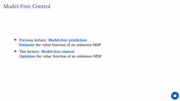
Model-Free Control

I Previous lecture: Model-free predictionEstimate the value function of an unknown MDP

I This lecture: Model-free controlOptimise the value function of an unknown MDP

Monte-Carlo Control

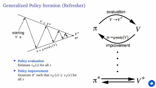
Generalized Policy Iteration (Refresher)

I Policy evaluationEstimate vπ(s) for all s

I Policy improvementGenerate π′ such that vπ′(s) ≥ vπ(s) forall s

Recap: Model-Free Policy Evaluation

vn+1(St ) = vn(St ) + α (Gt − vn(St ))

I Variants:

GMCt = Rt+1 + γRt+2 + γ

2Rt+3 + . . .

= Rt+1 + γGMCt+1 MC

G(1)t = Rt+1 + γvt (St+1) TD(0)

G(n)t = Rt+1 + γRt+2 + . . . + γn−1Rt+n + γ

nvt (St+n)

= Rt+1 + γG(n−1)t+1 n-step TD

Gλt = Rt+1 + γ[(1 − λ)vt (St+1) + λGλ

t+1] TD(λ)

In all cases, for given π goal is estimating vπ , data is generated to π

Model-Free Policy Iteration Using Action-Value Function

I Greedy policy improvement over v(s) requires model of MDP

π′(s) = argmaxa

E [Rt+1 + γv(St+1) | St = s, At = a]

I Greedy policy improvement over q(s, a) is model-free

π′(s) = argmaxa

q(s, a)

I This makes action values convenient

Generalised Policy Iteration with Action-Value Function

Starting Q, π

π = greedy(Q)

Q = Q π

Q*, π*

Policy evaluation Monte-Carlo policy evaluation, q ≈ qπ

Policy improvement Greedy policy improvement? No exploration!(Can’t sample all s, a, when learning by interacting)

Monte-Carlo Generalized Policy Iteration

Starting Q

π = ε-greedy(Q)

Q = Q π

Q*, π*

Every episode:Policy evaluation Monte-Carlo policy evaluation, q ≈ qπ

Policy improvement ε -greedy policy improvement

Model-free controlRepeat:I Sample episode 1, . . . , k, . . ., using π: {S1, A1, R2, ..., ST } ∼ πI For each state St and action At in the episode,

q(St, At ) ← q(St, At ) + αt (Gt − q(St, At ))

I E.g.,

αt =1

N(St, At )of αt = 1/k

I Improve policy based on new action-value function

ε ← 1/kπ ← ε -greedy(q)

(Generalises the ε -greedy bandit algorithm)

GLIE

DefinitionGreedy in the Limit with Infinite Exploration (GLIE)I All state-action pairs are explored infinitely many times,

∀s, a limt→∞

Nt (s, a) = ∞

I The policy converges to a greedy policy,

limt→∞

πt (a|s) = I(a = argmaxa′

qt (s, a′))

I For example, ε -greedy with εk = 1k

GLIE

TheoremGLIE Model-free control converges to the optimal action-value function, qt → q∗

Temporal-Difference LearningFor Control

MC vs. TD Control

I Temporal-difference (TD) learning has several advantages over Monte-Carlo (MC)I Lower variance

I Online

I Can learn from incomplete sequences

I Natural idea: use TD instead of MC for controlI Apply TD to q(s, a)I Use, e.g., ε -greedy policy improvement

I Update every time-step

Updating Action-Value Functions with SARSA

s,a

r

a'

s'

qt+1(St, At ) = qt (St, At ) + αt (Rt+1 + γq(St+1, At+1) − q(St, At ))

SARSA

Starting Q

π = ε-greedy(Q)

Q = Q π

Q*, π*

Every time-step:Policy evaluation SARSA, q ≈ qπPolicy improvement ε -greedy policy improvement

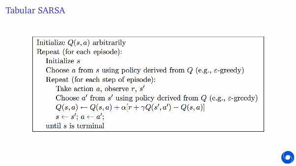
Tabular SARSA

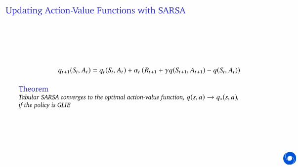
Updating Action-Value Functions with SARSA

qt+1(St, At ) = qt (St, At ) + αt (Rt+1 + γq(St+1, At+1) − q(St, At ))

TheoremTabular SARSA converges to the optimal action-value function, q(s, a) → q∗(s, a),if the policy is GLIE

Off-policy TD and Q-learning

Dynamic programming

I We discussed several dynamic programming algorithms

vk+1(s) = E [Rt+1 + γvk(St+1) | St = s, At ∼ π(St )] (policy evaluation)vk+1(s) = max

aE [Rt+1 + γvk(St+1) | St = s, At = a] (value iteration)

qk+1(s, a) = E [Rt+1 + γqk(St+1, At+1) | St = s, At = a] (policy evaluation)

qk+1(s, a) = E[Rt+1 + γmax

a′qk(St+1, a′) | St = s, At = a

](value iteration)

TD learning

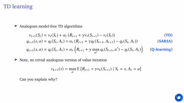
I Analogous model-free TD algorithms

vt+1(St ) = vt (St ) + αt (Rt+1 + γvt (St+1) − vt (St )) (TD)qt+1(s, a) = qt (St, At ) + αt (Rt+1 + γqt (St+1, At+1) − qt (St, At )) (SARSA)

qt+1(s, a) = qt (St, At ) + αt

(Rt+1 + γmax

a′qt (St+1, a′) − qt (St, At )

)(Q-learning)

I Note, no trivial analogous version of value iteration

vk+1(s) = maxa

E [Rt+1 + γvk(St+1) | St = s, At = a]

Can you explain why?

On and Off-Policy Learning

I On-policy learningI Learn about behaviour policy π from experience sampled from π

I Off-policy learningI Learn about target policy π from experience sampled from µ

I Learn ‘counterfactually’ about other things you could do: “what if...?”

I E.g., “What if I would turn left?” =⇒ new observations, rewards?

I E.g., “What if I would play more defensively?” =⇒ different win probability?

I E.g., “What if I would continue to go forward?” =⇒ how long until I bump into a wall?

Off-Policy Learning

I Evaluate target policy π(a|s) to compute vπ(s) or qπ(s, a)I While using behaviour policy µ(a|s) to generate actionsI Why is this important?

I Learn from observing humans or other agents (e.g., from logged data)

I Re-use experience from old policies (e.g., from your own past experience)

I Learn about multiple policies while following one policy

I Learn about greedy policy while following exploratory policy

I Q-learning estimates the value of the greedy policy

qt+1(s, a) = qt (St, At ) + αt

(Rt+1 + γmax

a′qt (St+1, a′) − qt (St, At )

)Acting greedy all the time would not explore sufficiently

Q-Learning Control Algorithm

TheoremQ-learning control converges to the optimal action-value function, q→ q∗, as long as we takeeach action in each state infinitely often.

Note: no need for greedy behaviour!

Works for any policy that eventually selects all actions sufficiently often(Requires appropriately decaying step sizes

∑t αt = ∞,

∑t α

2t < ∞,

E.g., α = 1/tω , with ω ∈ (0.5, 1))

Example

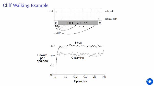
Cliff Walking Example

Overestimation in Q-learning

Q-learning overestimation

I Classical Q-learning has potential issuesI Recall

maxa

qt (St+1, a) = qt (St+1, argmaxa

qt (St+1, a))

I Uses same values to select and to evaluateI ... but values are approximate

I more likely to select overestimated values

I less likely to select underestimated values

I This causes upward bias

Q-learning overestimation: roulette example

I Roulette: gambling gameI Here, 171 actions: bet $1 on one of 170 options, or ‘stop’I ‘Stop’ ends the episode, with $0I All other actions have high variance reward, with negative expected valueI Betting actions do not end the episode, instead can bet again

Q-learning overestimation: roulette exampleI Roulette: gambling gameI Here, 171 actions: bet $1 on one of 170 options, or ‘stop’I ‘Stop’ ends the episode, with $0I All other actions have high variance reward, with negative expected valueI Betting actions do not end the episode, instead can bet again

Q-learning overestimation

I Q-learning overestimates because it uses the same values to select and to evaluate

maxa

qt (St+1, a) = qt (St+1, argmaxa

qt (St+1, a))

I Roulette: quite likely that some actions have won, on average

I Q-learning will updates if the state actually has high value

I Solution: decouple selection from evaluation

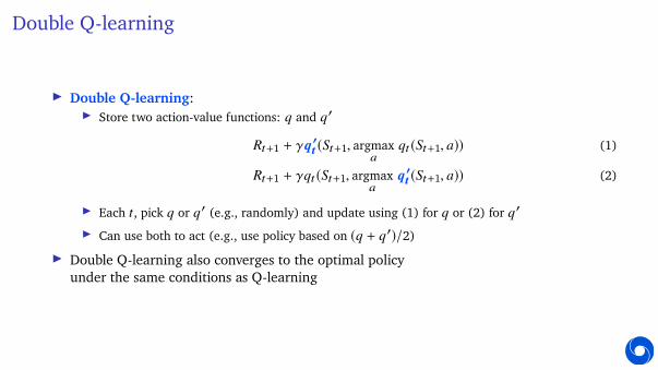
Double Q-learning

I Double Q-learning:I Store two action-value functions: q and q′

Rt+1 + γq′t (St+1, argmax

aqt (St+1, a)) (1)

Rt+1 + γqt (St+1, argmaxa

q′t (St+1, a)) (2)

I Each t, pick q or q′ (e.g., randomly) and update using (1) for q or (2) for q′

I Can use both to act (e.g., use policy based on (q + q′)/2)

I Double Q-learning also converges to the optimal policyunder the same conditions as Q-learning

Roulette example

Double DQN on Atari

DQNDouble DQN(This used a ‘target network’,to be explained later)

0 100

200

400

800

1600

3200

6400

Normalized score

Hum

an

Double DunkWizard of Wor

Video PinballGravitar

Private EyeAsterix

AsteroidsMontezuma's Revenge

FrostbiteVenture

Ms. PacmanZaxxonBowling

SeaquestAlien

AmidarTutankhamCentipede

Bank HeistRiver Raid

Up and DownChopper Command

Q*BertH.E.R.O.

Battle ZoneKung-Fu Master

Beam RiderIce Hockey

EnduroName This Game

Fishing DerbyJames Bond

KangarooSpace Invaders

Time PilotFreeway

PongGopherTennis

Road RunnerCrazy Climber

BoxingKrull

Star GunnerDemon Attack

AtlantisAssault

RobotankBreakout

Double learning

I The idea of double Q-learning can be generalised to other updatesI E.g., if you are (soft-) greedy (e.g., ε -greedy), then SARSA can also overestimate

I The same solution can be used

I =⇒ double SARSA

Example

Off-Policy Learning:Importance Sampling Corrections

Off-policy learning

I Recall: off-policy learning means learning about one policy π from experience generatedaccording to a different policy µ

I Q-learning is one example, but there are other optionsI Fortunately, there are general tools to help with thisI Caveat: you can’t expect to learn about things you never do

Importance sampling corrections

I Goal: given some function f with random inputs X , and a distribution d ′,estimate the expectation of f (X) under a different (target) distribution d

I Solution: weight the data by the ration d/d ′

Ex∼d[ f (x)] =∑

d(x) f (x)

=∑

d ′(x)d(x)d ′(x)

f (x)

= Ex∼d′

[d(x)d ′(x)

f (x)]

I Intuition:I scale up events that are rare under d′, but common under dI scale down events that are common under d′, but rare under d

Importance sampling corrections

I Example: estimate one-step rewardI Behaviour is µ(a|s)

E [Rt+1 | St = s, At ∼ π] =∑a

π(a|s)r(s, a)

=∑

µ(a|s)π(a|s)µ(a|s)

r(s, a)

= E

[π(At |St )µ(At |St )

Rt+1 | St = s, At ∼ µ

]I Ergo, when following policy µ, can use π(At |St )

µ(At |St )Rt+1 as unbiased sample

Importance Sampling for Off-Policy Monte-Carlo

I Goal: estimate vπI Data: trajectory τt = {St, At, Rt+1, St+1, . . .} generated with µI Solution: use return G(τt ) = Gt = Rt+1 + γRt+2 + . . ., and correct:

p(τt |π)p(τt |µ)

G(τt ) =p(At |St, π)p(Rt+1, St+1 |St, At )p(At+1 |St+1, π) · · ·p(At |St, µ)p(Rt+1, St+1 |St, At )p(At+1 |St+1, µ) · · ·

Gt

=p(At |St, π)(((((((((

p(Rt+1, St+1 |St, At )p(At+1 |St+1, π) · · ·

p(At |St, µ)(((((((((p(Rt+1, St+1 |St, At )p(At+1 |St+1, µ) · · ·

Gt

=p(At |St, π)p(At+1 |St+1, π) · · ·p(At |St, µ)p(At+1 |St+1, µ) · · ·

Gt

=π(At |St )µ(At |St )

π(At+1 |St+1)µ(At+1 |St+1)

· · ·Gt

Importance Sampling for Off-Policy TD Updates

I Use TD targets generated from µ to evaluate πI Weight TD target r + γv(s′) by importance samplingI Only need a single importance sampling correction

v(St ) ← v(St ) + α(π(At |St)µ(At |St)

(Rt+1 + γv(St+1)) − v(St ))

I Much lower variance than Monte-Carlo importance samplingI Policies only need to be similar over a single step

Importance Sampling for Off-Policy TD UpdatesI Proof:

Eµ

[π(At |St )µ(At |St )

(Rt+1 + γv(St+1)) − v(St )���� St = s

]=

∑a

µ(a|s)(π(a|s)µ(a|s)

E[Rt+1 + γv(St+1)|St = s, At = a] − v(s))

=∑a

π(a|s)E[Rt+1 + γv(St+1) | St = s, At = a] −∑a

µ(a|s)v(s)

=∑a

π(a|s)E[Rt+1 + γv(St+1) | St = s, At = a] −∑a

π(a|s)v(s)

=∑a

π(a|s)(E[Rt+1 + γv(St+1) | St = s, At = a] − v(s)

)= Eπ

[Rt+1 + γv(St+1) − v(s) | St = s

]

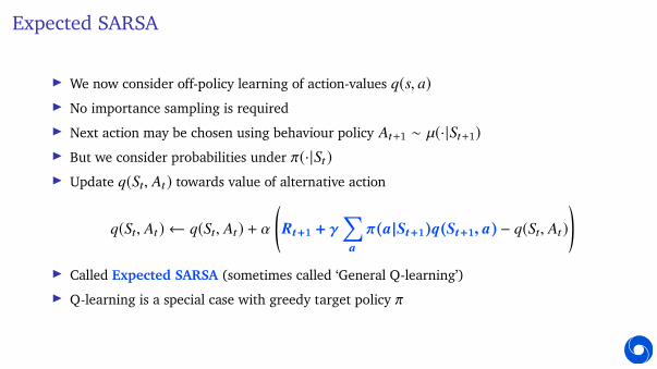
Expected SARSA

I We now consider off-policy learning of action-values q(s, a)I No importance sampling is requiredI Next action may be chosen using behaviour policy At+1 ∼ µ(·|St+1)I But we consider probabilities under π(·|St )I Update q(St, At ) towards value of alternative action

q(St, At ) ← q(St, At ) + α

(Rt+1 + γ

∑

a

π(a|St+1)q(St+1, a) − q(St, At )

)I Called Expected SARSA (sometimes called ‘General Q-learning’)I Q-learning is a special case with greedy target policy π

Summary

Model-Free Policy Iteration

I We can learn action values to predict the current policy πI Then we can do policy improvement, e.g., make the policy greedy π → π′

I Q-learning is akin to value iteration: immediately estimate the current greedy policyI (Expected) SARSA can be used more similar to policy iteration:

evaluate current behaviour, then (immediately) update behaviourI Sometimes we want to estimate some different policy: this is off-policy learningI Learning about the greedy policy is a special case of off-policy learning

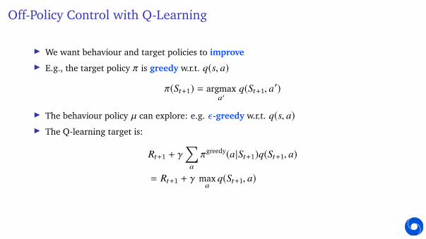
Off-Policy Control with Q-Learning

I We want behaviour and target policies to improveI E.g., the target policy π is greedy w.r.t. q(s, a)

π(St+1) = argmaxa′

q(St+1, a′)

I The behaviour policy µ can explore: e.g. ε -greedy w.r.t. q(s, a)I The Q-learning target is:

Rt+1 + γ∑a

πgreedy(a|St+1)q(St+1, a)

= Rt+1 + γ maxa

q(St+1, a)

On-Policy Control with SARSA

I In SARSA, the target and behaviour policies are the same

target = Rt+1 + γq(St+1, At+1)

I Then, for convergence to q∗, we need the addition requirement that π becomes greedyI For instance, ε -greedy or softmax with decreasing exploration

Summary

I Q-learning uses a greedy target policyI SARSA uses a stochastic sample from the behaviour as target policyI Expected SARSA uses any target policyI Double learning uses a separate value function to evaluate the policy (for any policy)I Double learning is not necessary is there is no correlation between target policy and value

function (e.g., pure prediction)I When using a greedy policy (Q-learning), there are strong correlations. Then double

learning (Double Q-learning) can be useful

Please use Moodle to ask questions

The only stupid question is the one you were afraid to ask but never did.-Rich Sutton