Lecture 6: Feature Detection

CAP 5415: Computer Vision

Fall 2009

In the text

• Today's material roughly matches Chapter 4 of the text

Feature Detection

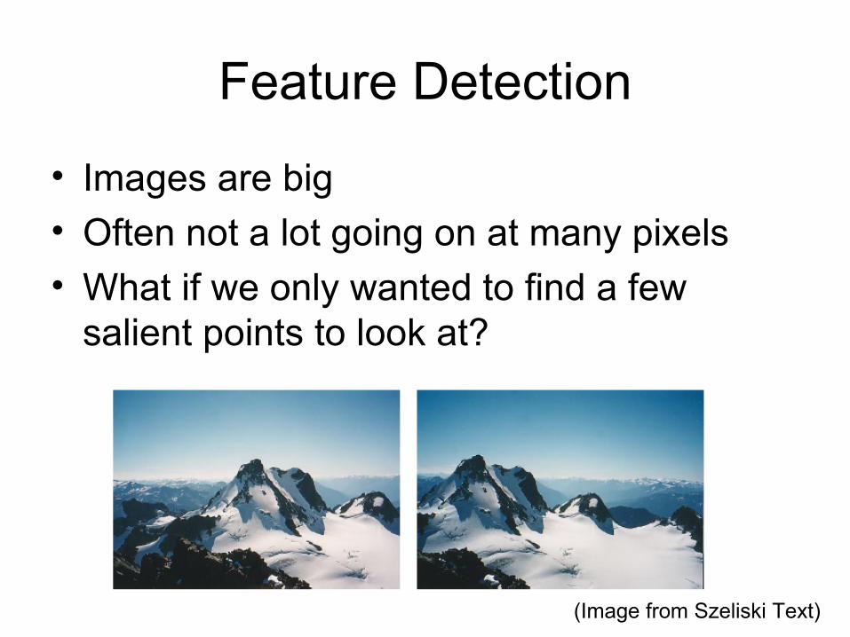
• Images are big

• Often not a lot going on at many pixels

• What if we only wanted to find a few salient points to look at?

(Image from Szeliski Text)

Feature Detection

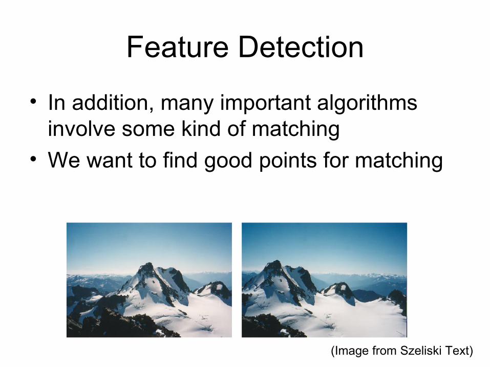
• In addition, many important algorithms involve some kind of matching

• We want to find good points for matching

(Image from Szeliski Text)

Today's Lecture

• Feature Point Detection– We will use the task of finding matching points

to motivate how points are selected

• Edge Detection

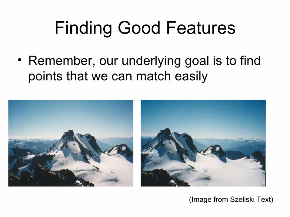
Finding Good Features

• Remember, our underlying goal is to find points that we can match easily

(Image from Szeliski Text)

Finding Good Features

• Would this be a good point to match?

(Image from Szeliski Text)

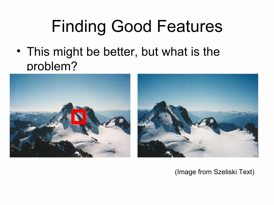
Finding Good Features• This might be better, but what is the

problem?

(Image from Szeliski Text)

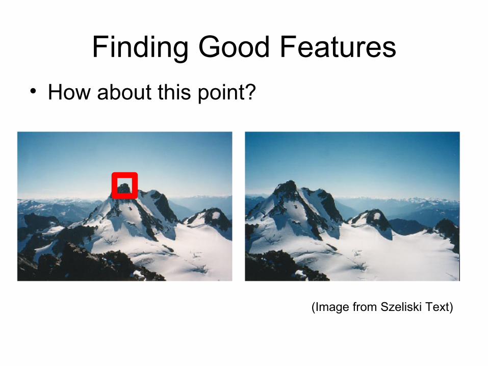
Finding Good Features• How about this point?

(Image from Szeliski Text)

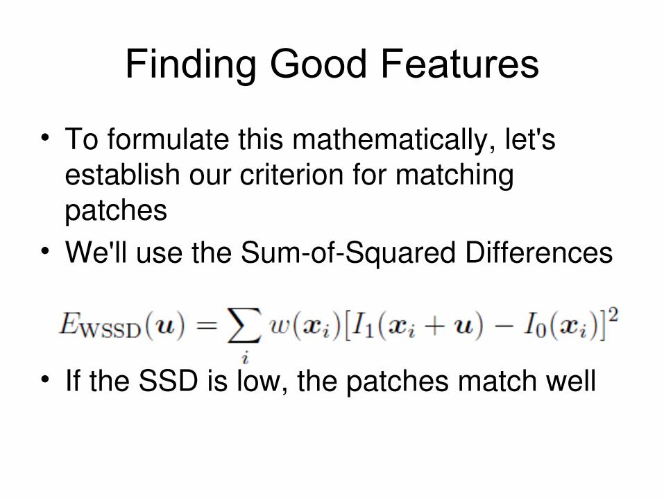
Finding Good Features

• To formulate this mathematically, let's establish our criterion for matching patches

• We'll use the Sum-of-Squared Differences

• If the SSD is low, the patches match well

But wait!

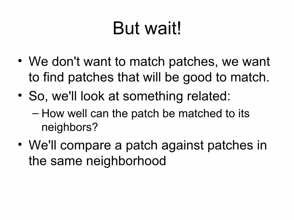
• We don't want to match patches, we want to find patches that will be good to match.

• So, we'll look at something related:– How well can the patch be matched to its

neighbors?

• We'll compare a patch against patches in the same neighborhood

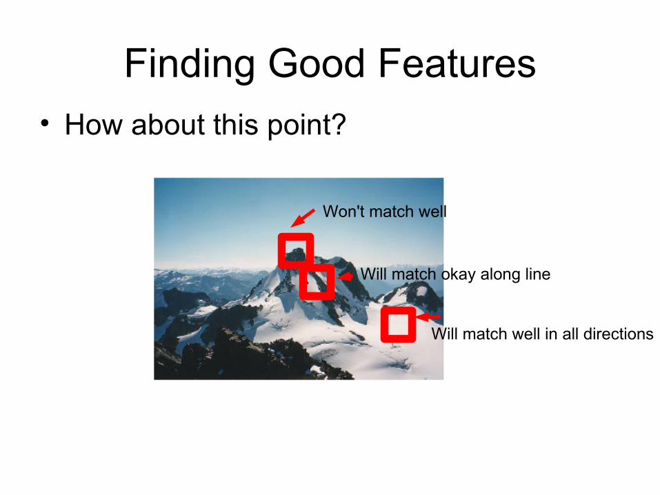
Finding Good Features• How about this point?

Won't match well

Will match okay along line

Will match well in all directions

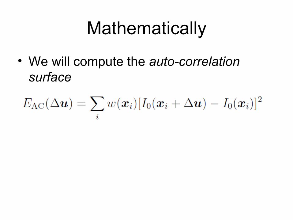
Mathematically

• We will compute the auto-correlation surface

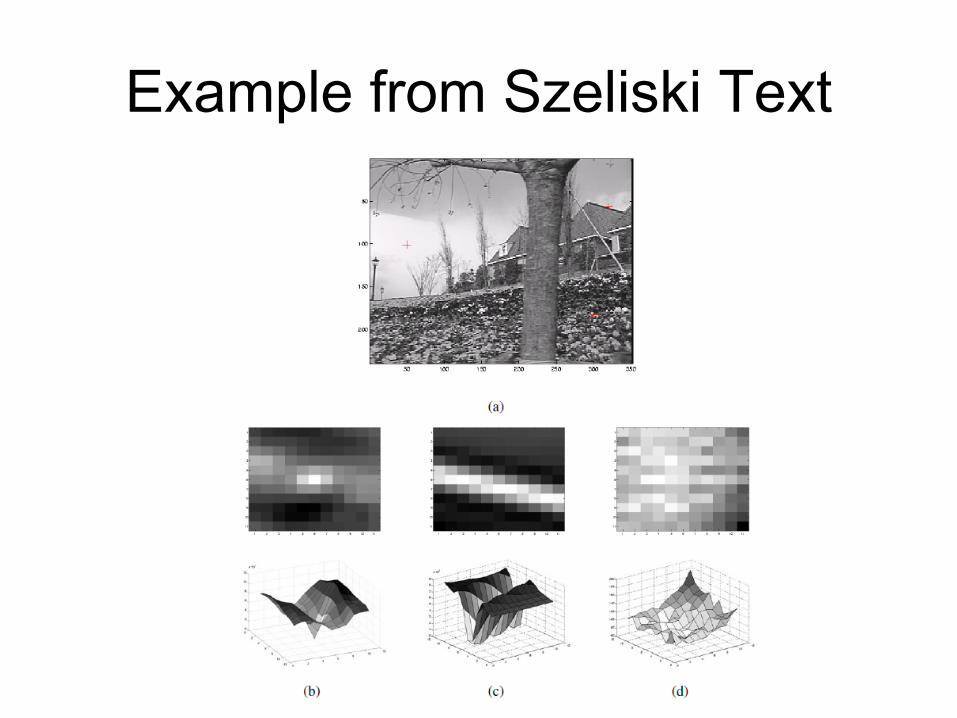
Example from Szeliski Text

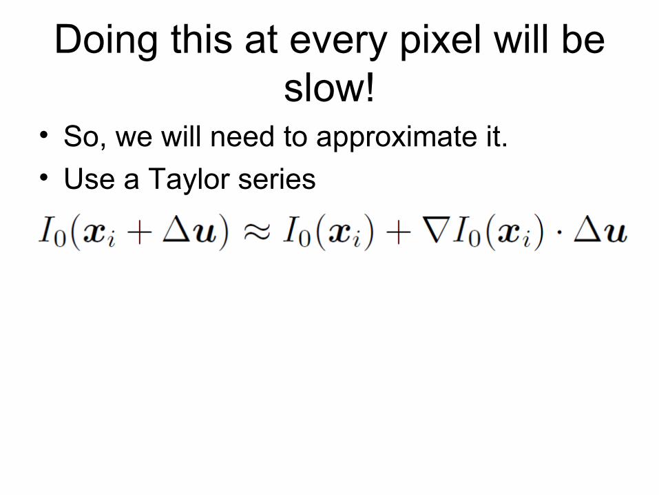
Doing this at every pixel will be slow!

• So, we will need to approximate it.

• Use a Taylor series

Now the auto-correlation surface becomes

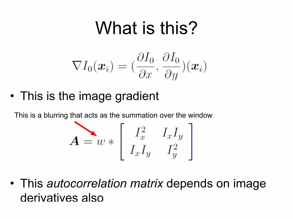
What is this?

• This is the image gradient

• This autocorrelation matrix depends on image derivatives also

This is a blurring that acts as the summation over the window

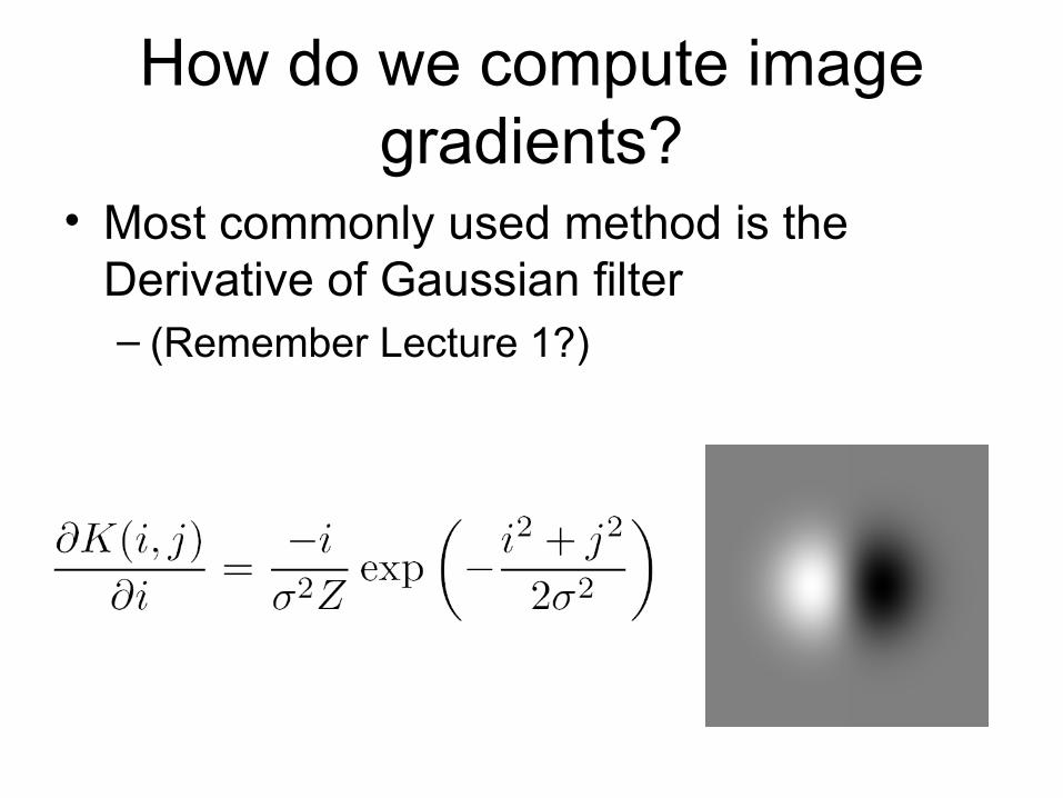
How do we compute image gradients?

• Most commonly used method is the Derivative of Gaussian filter– (Remember Lecture 1?)

Now,we need a number to tell us if this is a good point

• “Harris Corner Detector”

• Shi-Tomasi– Minimum Eigenvalue

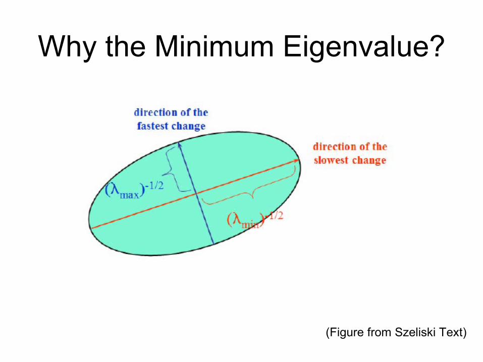
Why the Minimum Eigenvalue?

(Figure from Szeliski Text)

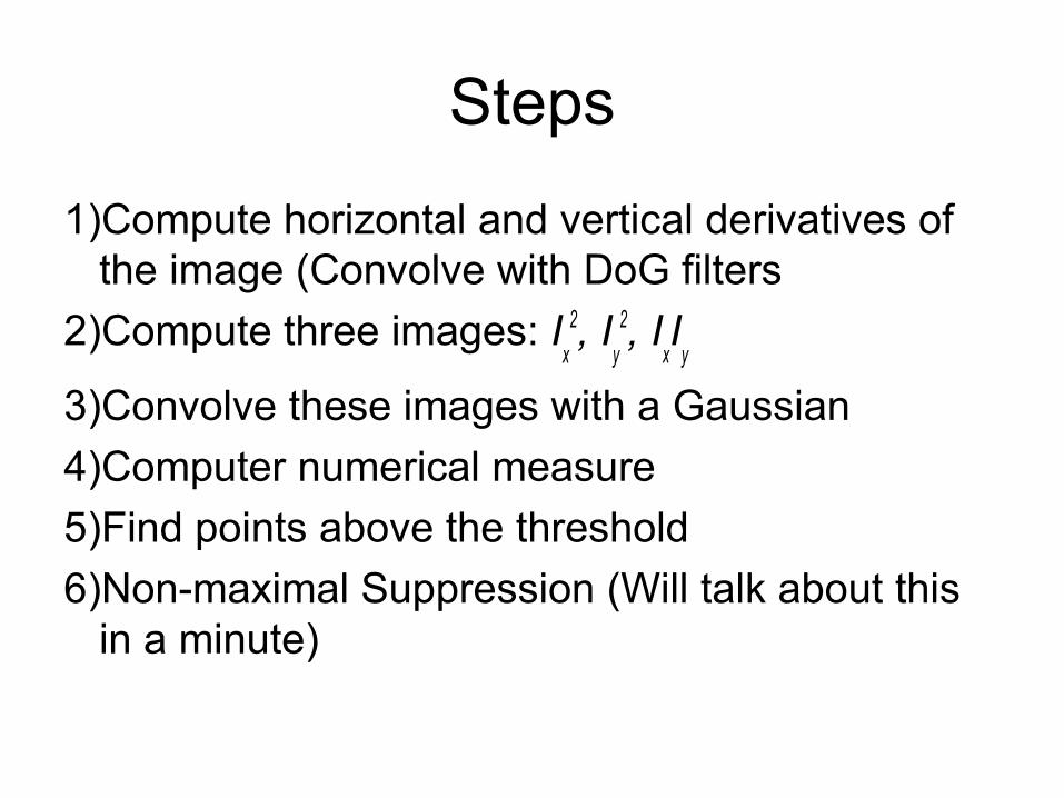
Steps

1)Compute horizontal and vertical derivatives of the image (Convolve with DoG filters

2)Compute three images: Ix

2, Iy

2, IxI

y

3)Convolve these images with a Gaussian

4)Computer numerical measure

5)Find points above the threshold

6)Non-maximal Suppression (Will talk about this in a minute)

Note

• These feature detectors are not just used where matching is important

• They are also

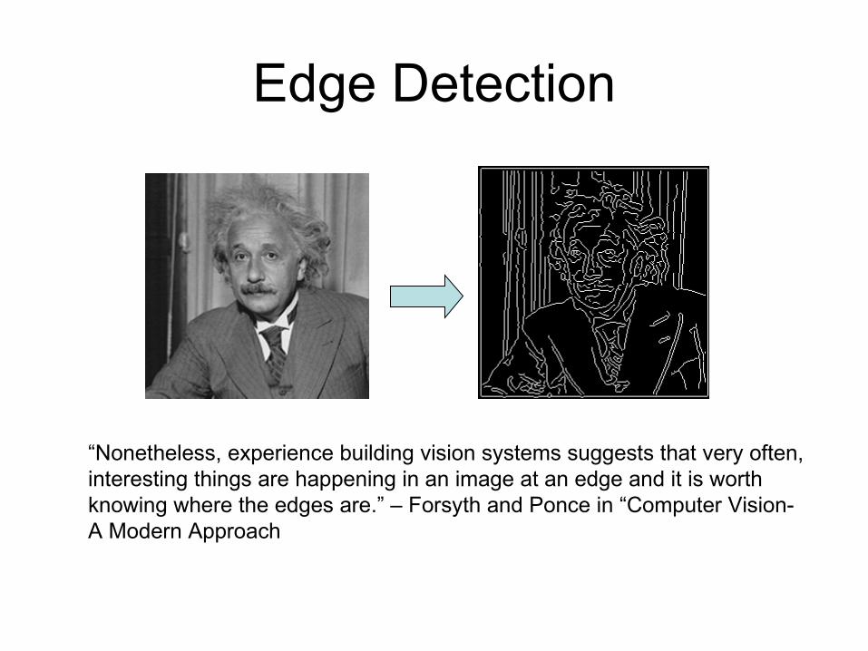
Edge Detection

“Nonetheless, experience building vision systems suggests that very often, interesting things are happening in an image at an edge and it is worth knowing where the edges are.” – Forsyth and Ponce in “Computer Vision- A Modern Approach

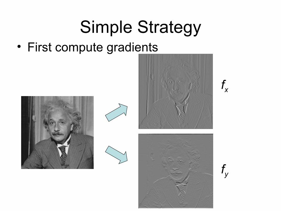
Simple Strategy• First compute gradients

fx

fy

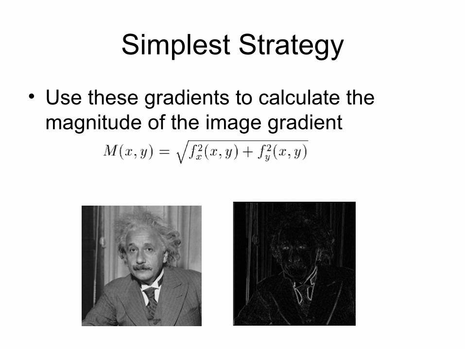
Simplest Strategy

• Use these gradients to calculate the magnitude of the image gradient

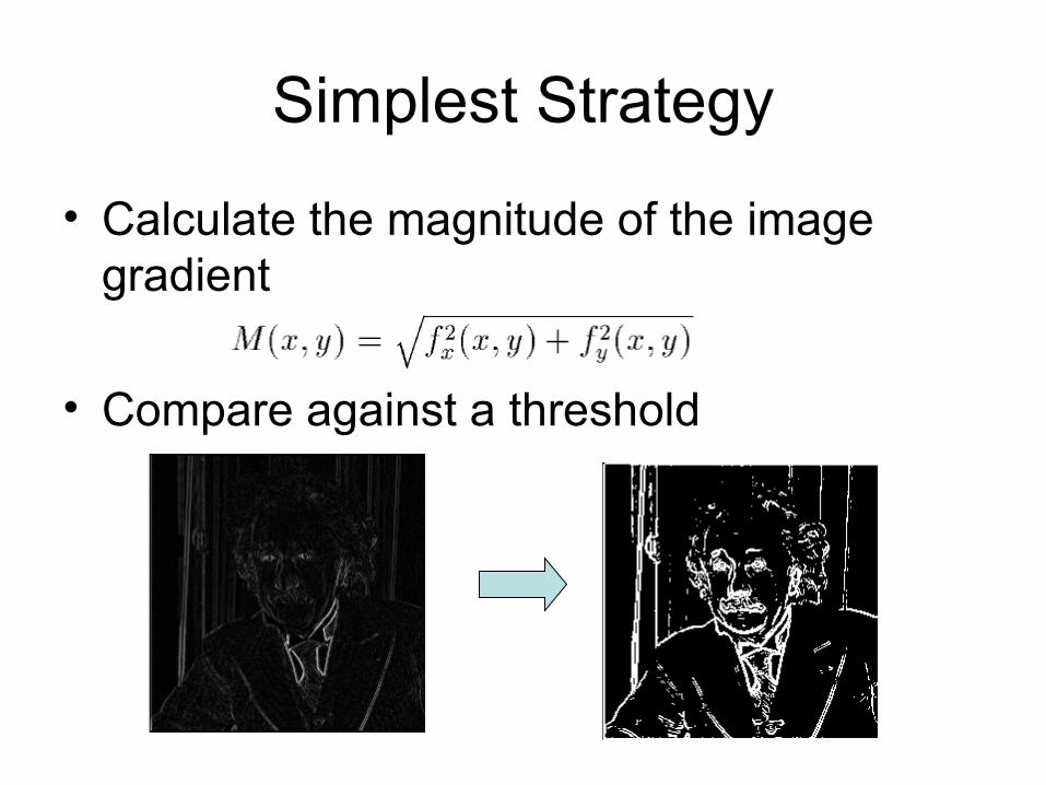
Simplest Strategy

• Calculate the magnitude of the image gradient

• Compare against a threshold

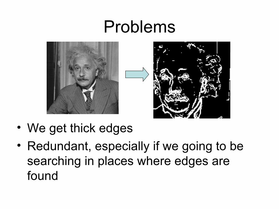
Problems

• We get thick edges

• Redundant, especially if we going to be searching in places where edges are found

Solution

• Identify the local maximums

• Called “non-maximal suppression”

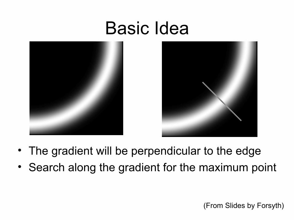
Basic Idea

• The gradient will be perpendicular to the edge• Search along the gradient for the maximum point

(From Slides by Forsyth)

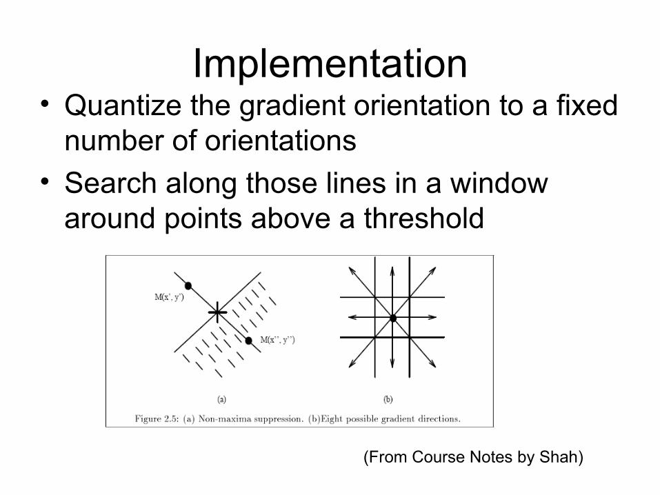
Implementation• Quantize the gradient orientation to a fixed

number of orientations

• Search along those lines in a window around points above a threshold

(From Course Notes by Shah)

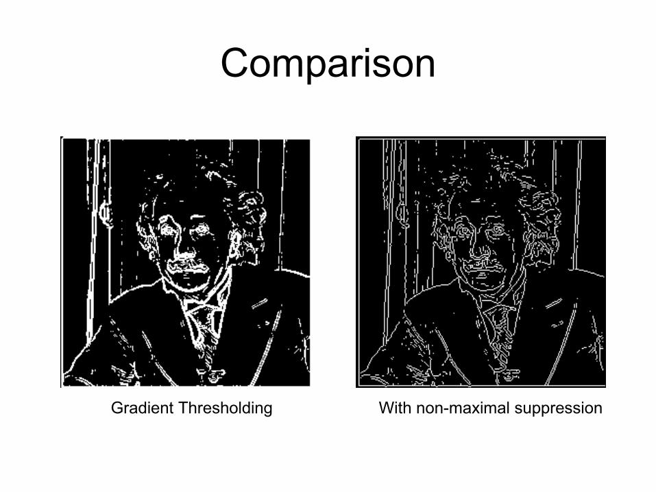
Comparison

Gradient Thresholding With non-maximal suppression

Avoiding Non-Maximal Suppression

• Can we formulate the problem so we can eliminate non-maximal suppression?

• Remember: we want to find the maxima and minima of the gradient

• Look for places where 2nd derivative is zero

• Called zero-crossings (you may not see the 2nd derivative actually be zero)

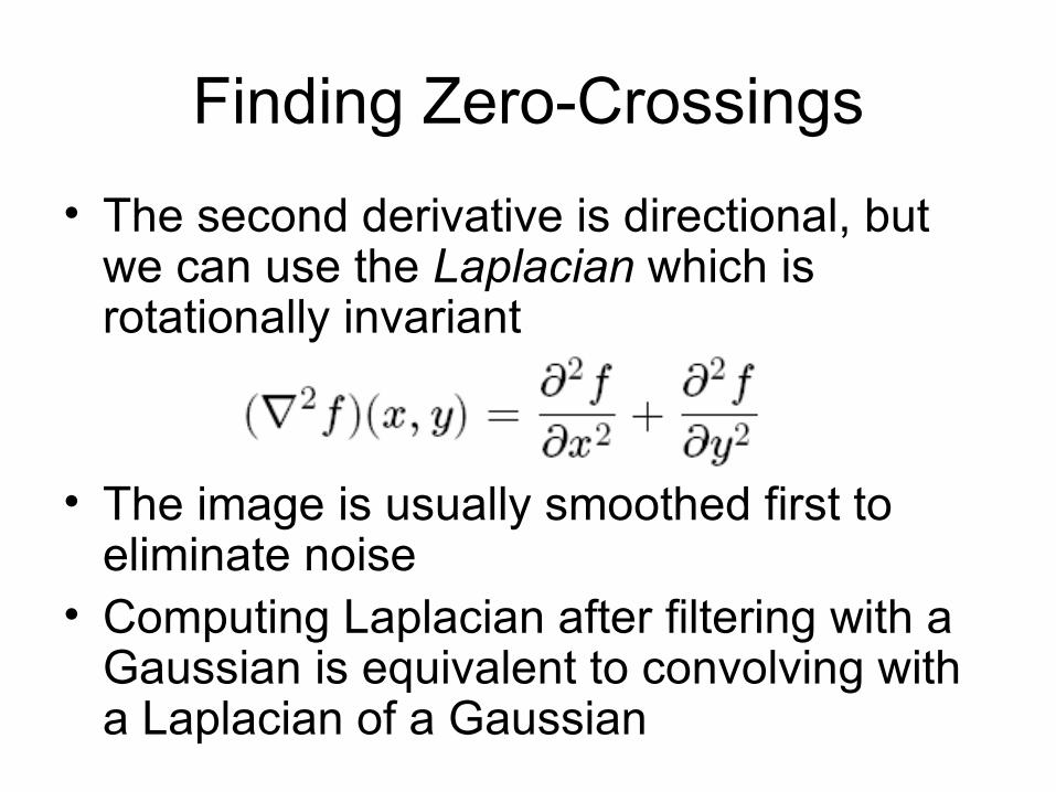
• The second derivative is directional, but we can use the Laplacian which is rotationally invariant

• The image is usually smoothed first to eliminate noise

• Computing Laplacian after filtering with a Gaussian is equivalent to convolving with a Laplacian of a Gaussian

Finding Zero-Crossings

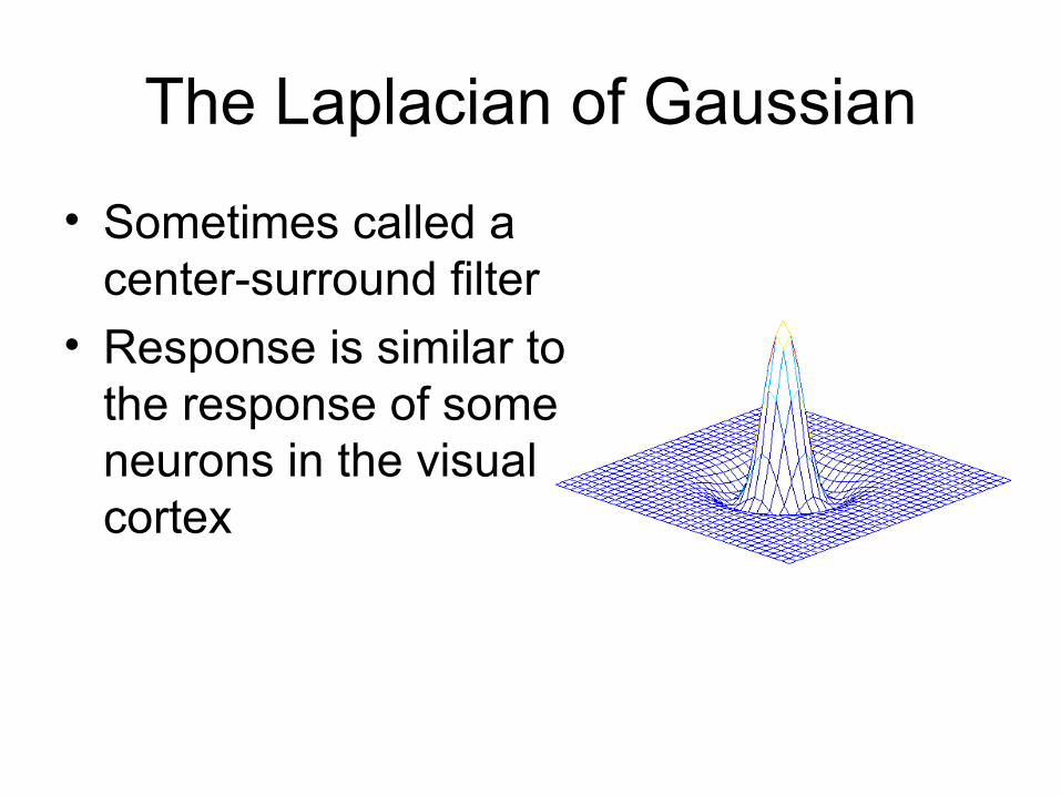
The Laplacian of Gaussian

• Sometimes called a center-surround filter

• Response is similar to the response of some neurons in the visual cortex

Implementation

• Filter with Laplacian of Gaussian

• Look for patterns like {+,0,-} or {+,-}

• Also known as the Marr-Hildreth Edge Detector

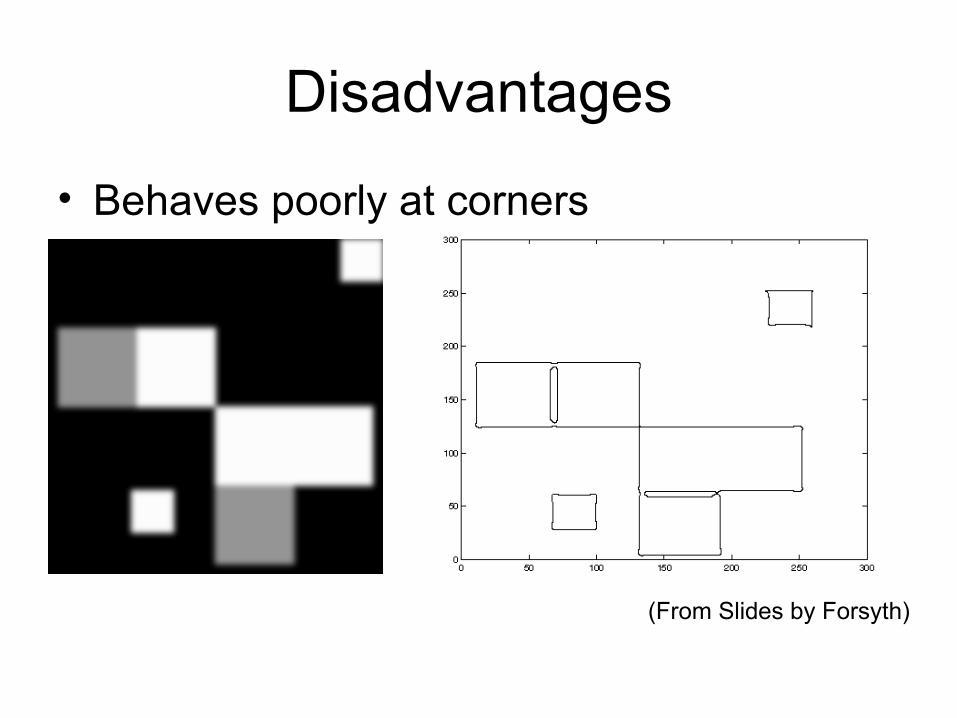
Disadvantages

• Behaves poorly at corners

(From Slides by Forsyth)

Noise and Edge Detection

• Noise is a bad thing for edge-detection– Usually assume that noise is white Gaussian

noise (not likely in reality!)

• Introduces many spurious edges

• Low-pass filtering is a simple way of reducing the noise– For the Laplacian of Gaussian Method, it is

integrated into the edge detection

Why does filtering with a Gaussian reduce noise?

• Forsyth and Ponce’s explanation:

“Secondly, pixels will have a greater tendency to look like neighbouring pixels — ifwe take stationary additive Gaussian noise, and smooth it, the pixel values of theresulting signal are no longer independent. In some sense, this is what smoothingwas about — recall we introduced smoothing as a method to predict a pixel’svalue from the values of its neighbours. However, if pixels tend to look like theirneighbours, then derivatives must be smaller (because they measure the tendencyof pixels to look different from their neighbours).”

– from Computer Vision – A Modern Approach

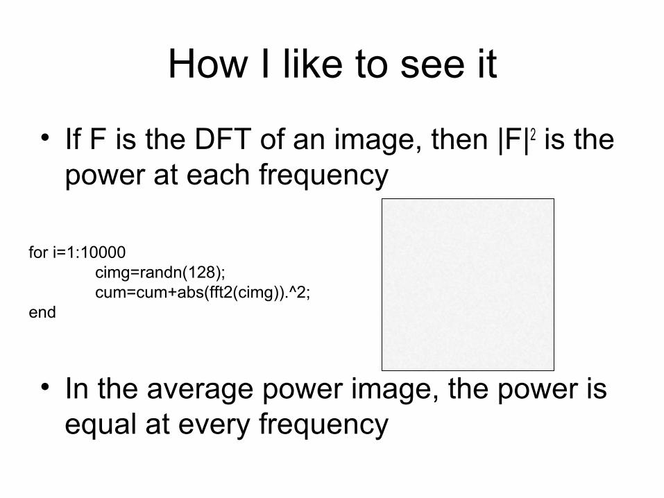
How I like to see it

• If F is the DFT of an image, then |F|2 is the power at each frequency

• In the average power image, the power is equal at every frequency

for i=1:10000cimg=randn(128);cum=cum+abs(fft2(cimg)).^2;

end

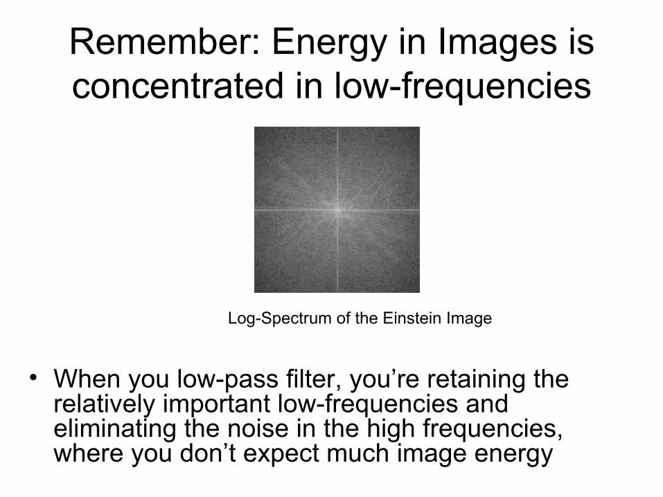
Remember: Energy in Images is concentrated in low-frequencies

• When you low-pass filter, you’re retaining the relatively important low-frequencies and eliminating the noise in the high frequencies, where you don’t expect much image energy

Log-Spectrum of the Einstein Image

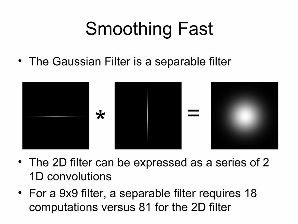
Smoothing Fast

• The Gaussian Filter is a separable filter

• The 2D filter can be expressed as a series of 2 1D convolutions

• For a 9x9 filter, a separable filter requires 18 computations versus 81 for the 2D filter

* =

Further Improvements to the Gradient Edge-Dector

• Fundamental Steps in Gradient-Based Edge Detection that we have talked about:– Smooth to reduce noise– Compute Gradients– Do Non-maximal suppression

• There is one more heuristic that we can advantage of.

• Edges tend to be continuous

Hysteresis Thresholding

• Edges tend to be continuous

• Still threshold the gradient

• Use a lower threshold if a neighboring point is an edge

• The “Canny Edge Detector” uses all of these heuristics

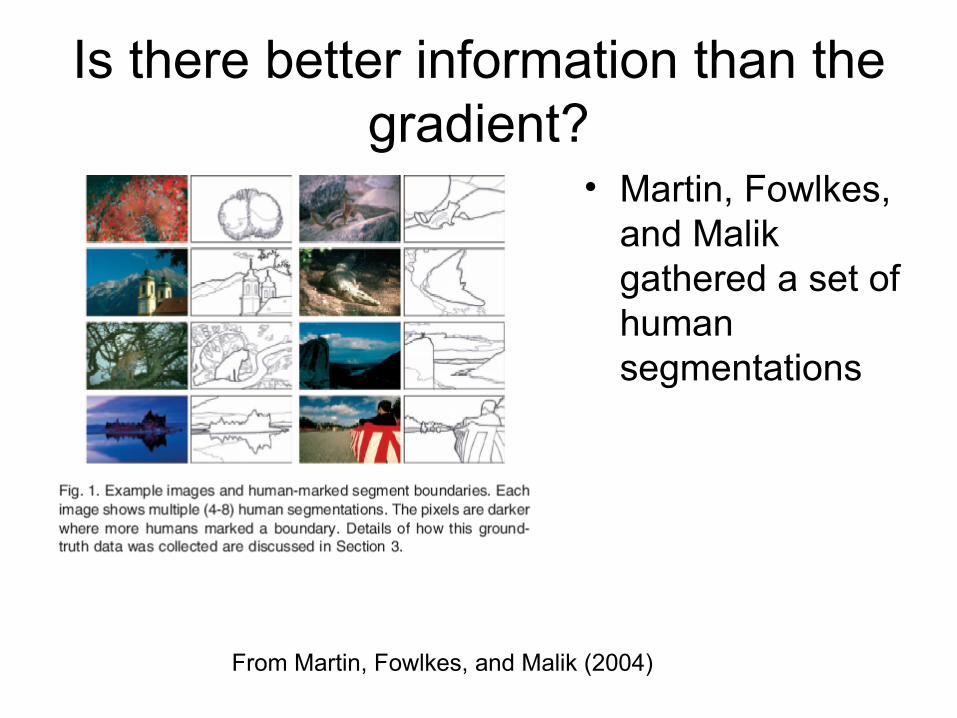
Is there better information than the gradient?

• Martin, Fowlkes, and Malik gathered a set of human segmentations

From Martin, Fowlkes, and Malik (2004)

Capturing Texture

Texture and Color Help

• This is a precision-recall curve

• The highest curve has the best performance

• The best performance comes from using brightness (Image gradient), texture and color

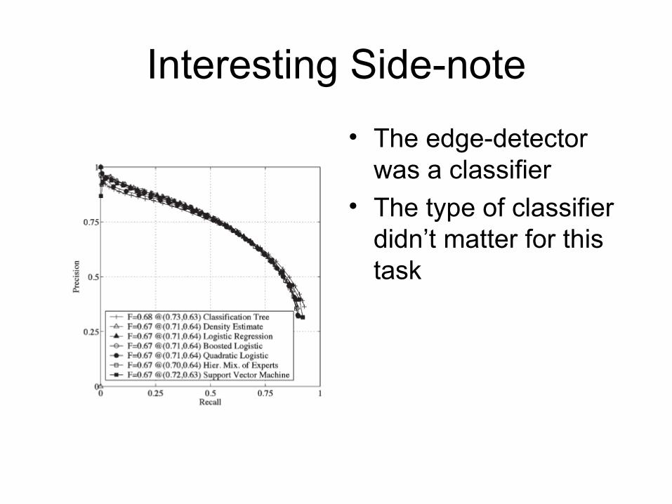
Interesting Side-note

• The edge-detector was a classifier

• The type of classifier didn’t matter for this task

• Next Time:– We’ll start talking about learning to classify

things like edges