8/11/2011

1

Lecture 5: Rules of Differentiation

Fi t d d i ti• First order derivatives• Higher order derivatives• Partial differentiation• Higher order partials• Differentials• Derivatives of implicit functionsDerivatives of implicit functions• Generalized implicit function theorem• Exponential and logarithmic functions• Taylor series approximation

First Order Derivatives

• Consider functions of a single independent i bl f X R X i t l f Rvariable, f : X R, X an open interval of R.

R1(constant function) f(x) = k f'(x) = 0.

R2 (power function) f(x) = xn f'(x) = nxn-1

R3 (multiplicative constant) f(x) = kg(x) f'(x) = kg'(x).

8/11/2011

2

Examples R1-R3

#1 Let y = f(x) = x3 . Find dy / dx x3 = (x)1/ 3. Hence, d / dx (x)1/3 =

1/3(x)1/3-1 = 1/3(x)-2/3 .

#2 Let y = f(x) = 3, where f: R+ R. Find dy /dx = 0

#3 Let y = f(x) = 10x0. Find dy / dx = (10) x0-1 = 0 1x = 0. = 0

#4 Let y = f(x) = 20 x4/5. Find dy /dx = 16x-1/5.

Two or more functions of the same variable: sum-difference

• Def 1. By the sum (difference) of any two l l d f ti f( ) d ( ) hreal-valued functions f(x) and g(x), where

f: D R and g: E R, we mean the real-valued function f g: D E R whose value at any x D E is the sum (difference) of two real numbers f(x) and g(x). In symbols we have

(f g) (x) = f(x) g(x), for any x D E.

8/11/2011

3

Rules

R4 (sum-difference) g(x) = i fi(x) g'(x) =

i fi'(x).

Remark: To account for differences, simply multiply any of the fi by -1 and use the multiplicative constant rulemultiplicative constant rule.

Examples

#1 What is the slope of the curve y= f(x) = x3 - 3x + 5, when it crosses the y

-axis?

First find

dydx

ddx

xddx

xd

dx 3 3 5

dy / dx = 3x2 - 3 = f(x).

h h h i h l When the curve crosses the y - axis, we have x = 0. Hence, evaluate

f(x) for x = 0.

f(0) = -3 .

Thus the slope at x = 0 is -3.

8/11/2011

4

Examples

#2 Find f(x) if f(x) = .5x7x

x 2/12

3

x

Clearly we may write f(x) as

f(x) = x -7x -1/2 + 5

Hence

f(x) = d

dxx

d

dxx

d

dx 7 51 2/

dx dx dx

f(x) = 1 + 72

x -3/2

Product

• Def By the product of any two real valued f ti f( ) d ( ) h f D Rfunctions f(x) and g(x), where f: D R and g: E R, we mean the real function

fg : D E R

whose value at any x D E is the product of the two real numbers f(x) andproduct of the two real numbers f(x) and g(x).

8/11/2011

5

Product Rule

R5 (product) h(x) = f(x)g(x) h'(x) = f'(x)g(x) + f(x)g'(x)

Remark: This rule can be generalized as

d[f1(x) f2(x) fN(x)] = f1(x)[f2(x) f3(x) fN(x)] + f2(x)[f1(x) f3(x) fN(x)]

dx[f1(x) f2(x) fN(x)] f 1(x)[f2(x) f3(x) fN(x)] + f 2(x)[f1(x) f3(x) fN(x)]

+ + fN(x)[f1(x) f2(x) fN-1(x)].

ExampleLet f(x) = x x

5

52 (5x + 6)

Findd

f(x) H ere we may consider f(x) as the product of twoFind dx

f(x). H ere we may consider f(x) as the product of two

functions, say

h(x) = x x5

52 , and g(x) = (5x + 6).

Hence d

dxf(x) =

d h x g x

dx

. U sing the product rule w e obtain

f(x) = (x4 + 2x) (5x +6) + x5 + 5x2

= x45x + 6x4 + 10x2 + 12x + x5 + 5x2

= x55 + 6x4 + 15x2 + 12x +x5

f (x) = 6x5 + 6x4 + 15x2 + 12x.

8/11/2011

6

Quotient

• Def. The quotient of any two real-valued f ti f( ) d ( ) h f D Rfunctions f(x) and g(x), where f: D R, g: E R, is the real-valued function f/g: D E R, defined for g(x) 0, whose value at any x D E is the quotient of the two real numbers f(x) / g(x), g(x) 0.

Quotient Rule

• R6 (quotient) h(x) = f(x)/g(x)

h'(x) = [f'(x)g(x) – g'(x)f(x)]/[g(x)]2

8/11/2011

7

Examples

#1 Find f(x), where f(x) = x

g x

3

( ), g(x) differentiable fn of x.

g x( )

3 2 3

2

x g x g x x

g x

( ) ( )

( )

#2 Find d

dx

x x

x

( )( ),

2 3

2

1 4

where x 0

Here we must use the product rule and the quotient rule.

2 4 3 1 2 1 43 2 2 2 2 3

4

x x x x x x x x

x

( ) ( ) ( )( )

Composite functions

Def The composite function of any two functions z = f(y) and y = g(x), where

X Y Zg f

such that the domain of f coincides with the range of g, is a function h(x), where

h : X Z,

defined by h(x) = f(g(x)) for every member x X

Remark: The notation f o g is used to denote the composite function f(g(x)).

defined by h(x) = f(g(x)) for every member x X.

8/11/2011

8

Example

• max u(x1,x2) st I = p1 x1 + p2 x2

• x2 = I/p2 - (p1/p2) x1 = g(x1)

• u(x1, I/p2 - (p1/p2) x1 ) = u(x1,g(x1))

• max u(x1,g(x1))

Example

Consider the two functions g: R R and f: R R defined by

y = g(x) = 3x -1

z = f(y) = 2y + 3

for any real numbers x, y. From our definition we may form the

function f g or f[g(x)]:

f g = f[g(x)] = 2(3x-1) + 3 = z,

where f g is defined for every real x.

8/11/2011

9

Composite function rule

• R7 (chain) If z = f(y) is a differentiable function of y and y = g(x) is a differentiablefunction of y and y = g(x) is a differentiable function of x, then the composite function f g or h(x) = f[g(x)] is a differentiable function of x and

h'(x) = f[g(x)] g(x).R k Thi l b t d d tRemark: This rule can be extended to any

finite chain. e.g., h = f(g(r(x))) h' = f'(g)g'(r)r'(x)

Examples

#1 Let z = 6y + 1/2y2 and y =3x. Theny y y

dz

dx=

dz

dy

dy

dx

=(6 + y)3

but y = 3x

dzdx

= (6 + 3x) 3 = 9x + 18

8/11/2011

10

Examples

#2 Let z = y

y

12 , y = 5x

y

dzdx

= 1 2 12

2 2

( ) ( )

( )

y y y

y

(5)

= 5 2 2 5 2 5 10 5 102 2

4

2

4

2

4 4

( ) ( ) ( )y y y

y

y y

y

y y

y

y y

y

dz

dx =

( )5 103

y

y

dx y

but y = 5x

dz

dx =

5 5x 10

5x 3

( )

( )

Inverse function

• Def. The inverse function of a function y = f( ) h f X Y i f ti f 1( )f(x), where f: X Y, is a function x = f-1(y), where f-1: f[X] X. We have that y = f(x) if and only if x = f-1(y) for all (x,y) Gr(f).

• Proposition If the function y = f(x) is one-• Proposition. If the function y = f(x) is one-to-one, then the inverse function x = f-1(y) exists.

8/11/2011

11

Inverse function

• A one-to-one function defined on real numbers is called monotonic A monotonicnumbers is called monotonic. A monotonic function is either increasing or decreasing.

• Def. A monotonic function f(x), f: R R is monotonically increasing iff for any x, x R, x > x implies f(x) > f(x).D f A t i f ti f( ) f R R i• Def. A monotonic function f(x), f: R R is a monotonically decreasing function iff for any x, x R, x > ximplies f(x) < f(x).

Inverse function

• Remark: A practical method of d t i i h th ti ldetermining whether a particular differentiable function is monotonic is to see if its derivative never changes sign. (> 0 if , < 0 if )

8/11/2011

12

Example

• Direct demand Q = D(p)

• Inverse demand p = D-1(Q) = p(Q)

• Q = 5-p. What is inverse demand?

Inverse function rule

• R8 (inverse function) Given y = f(x) and x f 1( ) h= f-1(y), we have

f-1'(y) = 1/f'(x).

• Proposition. If a function y = f(x), f : X Y, is one-to-one, then

(i) the inverse function x = f-1(y) exists(i) the inverse function x = f-1(y) exists,

(ii) f-1(y) is one-to-one,

(iii) (f-1)-1 = f.

8/11/2011

13

ExamplesLet y = f(x ) = 5x + 4, f: R R .

f i s b i jec tiv e f -1(y) .

y 4 f -1(y ) =

y 4

5 = x

N o w fin d d

d xf (x ) and

d

dyf -1( y) an d com p are .

d

dxf(x ) = 5 , th en b y in ver se f n ru le

d

dyf -1(y ) sh ou ld = 1/5 .

df - 1( y) =

( )1 5 0 5 1

dyf ( y)

25 25 5

F ro m ab o v e w e s ee th at

y = 5 x + 4

x = 15 y - 4 /5

a re b o th bij ec tiv e .

Higher Order Derivatives

• If a function is differentiable, then its derivative function is itself a function whichderivative function is itself a function which may possess a derivative.

• If this is the case, then the derivative function may be differentiated. This derivative is called the second derivative. If d i ti f th d d i ti• If a derivative of the second derivative function exists, then the resultant derivative is called the third derivative.

8/11/2011

14

Higher Order Derivatives

• Generally, if successive derivatives exist, a function may have any number of highera function may have any number of higher order derivatives.

• The second derivative is denoted f''(x) or d2f/dx2 and the nth order derivative is given by dnf/dxn.E l L t f( ) 3 5 10 W h• Example: Let f(x) = 3x5 + 10x. We have that f' = 15x4 + 10, f'' = 60x3, and d3f/dx3

= 180x2.

Partial derivatives

• Here we consider a function of the form

y = f(x1, , xn), f: Rn R.

• Short-hand notation: y = f(x), where x Rn.

8/11/2011

15

Partial derivative: definition

• Def. The partial derivative of the function f( ) f Rn R t i t ( of(x1,x2,, xn), f: Rn R, at a point (x1

o

,xo2,, xo

n) with respect to xi is given by

lim

( ,. .. , , , ) ( , , )

x

yx

oi i N N

i

f x x x x f x xx

0

10 0

10 0

xii x0

Notation

Notation: We denote the partial derivative, lim

x

yx

ii0, in each of the following ways.

fi(x), f(x)/xi or ix

f(x).

8/11/2011

16

Illustration

f

xo1

f

f1

xo2

Summary

The mechanics of differentiation are very i lsimple:

• When differentiating with respect to xi, regard all other independent variables as constants

• Use the simple rules of differentiation for• Use the simple rules of differentiation for xi.

8/11/2011

17

Examples

#1 Let y = f(x 1,x 2) = x 12 + x 2 + 3

then

f

x 1

= 2x1 and

f

x 2

= 1

#2 L et y = f(x 1, x 2 ,x 3) = (x 1 + 3 ) ( x 22 + 4 ) (x 3)

fx 1

= 1 ( x 22 + 4) (x3)

#3 L et y = f(x 1,x 2) = x x12

24 + 10x 1

f

x 1

= 2x 1 x 24 + 10

Extensions of the chain rule

a Let y = f(x1 xn) where xi = xi(x1) for i = 2 n We have thata. Let y f(x1,...,xn), where xi xi(x1), for i 2,...,n. We have that

dy/dx1 = f/x1 +

fxii

n

2

dxdx

i

1

.

b . L et y = f( x1,...,x n), w here i x i = x i(u ). T hen w e have that y ( , , ), ( )

dy /du = fdx

duii

i

n

1.

8/11/2011

18

Extensions of the chain rule

c. Let y = f(x1,...,xn), where xi = xi(v1,...,vm), for all i. Then we have that y ( ) ( )

y/vj = fxvi

i

ni

j

1

.

Example

• Let y = f(x1,x2) = 3x1 + x22, where x1 = v2

d 5 Fi d //+u and x2 = u + 5v. Find

vyuy /,/

8/11/2011

19

Higher order partial derivatives

• A first order partial derivative function is it lf f ti f th i d d titself a function of the n independent variables of the original function. Thus, if this function has partial derivatives, then we can define higher order partial derivative functions. Th t i t ti th d d• The most interesting are the second order partial derivative functions denoted

fij(x) = x Rn.ji xxf /2

Higher order partial derivatives

• If i and j are equal, then fii is called a direct second order partial derivative and if ij f issecond order partial derivative and if ij, fij is called a cross second order partial derivative.

• We can associate a matrix of partial derivatives to each point (x1,...,xn) in the domain of f. The matrix is defined by

H(xo) = [f (xo )]H(xo) = [fij(xo )]i,j = 1,…,n

and it is called the Hessian of f at the arbitrary point xo.

8/11/2011

20

Examples #1. Let f = (x1 + 3)(x2

2 + 4)x3. We have that

f1 = (x22 + 4)x3, f11 = 0, f12 = 2x2x3, f13 = (x2

2 + 4)

f2 = (x1 + 3)(x3)(2x2), f22 = 2(x1 + 3)x3, f21 = 2x2x3, f23 = (x1 + 3)(2x2).

f3 = (x1 + 3)(x22 + 4), f32 = (x1 + 3)(2x2), f31 = (x2

2 + 4), f33 = 0.

#2 . L et f = x 1x 2.

f1 = x 2, f12 = 1 , f11 = 0 ,

f2 = x 1, f21 = 1 , f22 = 0 .

The Hessian at any po in t (x 1,x 2) i s given by

H = 0 1

1 0

=

f f

f f11 12

21 22

.

A result

• Young's Theorem. If f(x), x Rn, ti ti l d i tipossesses continuous partial derivatives

at a point, then fij = fji at that point.

• Example: f = x2y2. Show fxy = fyx.

8/11/2011

21

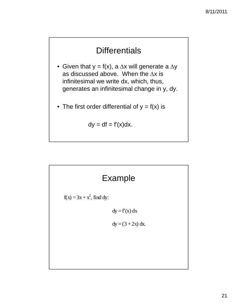
Differentials

• Given that y = f(x), a x will generate a y di d b Wh th ias discussed above. When the x is

infinitesimal we write dx, which, thus, generates an infinitesimal change in y, dy.

• The first order differential of y = f(x) is• The first order differential of y = f(x) is

dy = df = f'(x)dx.

Example

f(x) = 3x + x2, find dy:( ) , y

dy = f(x) dx

dy = (3 + 2x) dx.

8/11/2011

22

Functions of Many Variables

• Given y = f(x1,…xn), the differential of f is i bgiven by

df = ifi (x) dxi.

Some rules

Proposition 1. If f(x1, x2, , xn) and g(x1, x2, , xn) are differentiable functions of the variables

xi ( i = 1, , n), then

(i) d (fn) = nfn-1df

(ii) d (f g) = df dg

(iii) d (f g) = gdf + fdg

f

gdf fdg (iv) d

f

g

=

gdf fdg

g 2, g 0.

8/11/2011

23

Example

• Let f = (x12 + 3x2)/x1x2, find df.

df = x x x

x xdx

xx x

dx12

2 22

1 22 1

13

1 22 2

3

( ) ( ).

2nd order differential

• It is also possible to take a differential of a fi t d diff ti l t d fifirst order differential so as to define a second order differential.

We have that d2f can be expressed as a

d2f =

n

1i

n

1i

fijdxidxj.

j=1i=1

• We have that d2f can be expressed as a quadratic form in dx:

dx'Hdx,

8/11/2011

24

Derivatives of Implicit Functions

• Implicit relationships between two variables x and y are often expressed asvariables x and y are often expressed as equations of the form

F(x, y) = 0. If possible, we would like to define explicit functions say x = x(y) and y = y(x) from thi l tithis relation.

• We would also like to define the derivatives of such functions.

Example

• A circle with radius 2 and center 0:

F(x, y) = x2 + y2 – 4 = 0.

y

2 2

2x 2 + y 2 - 4 = 0

x 2

- 2

- 2

8/11/2011

25

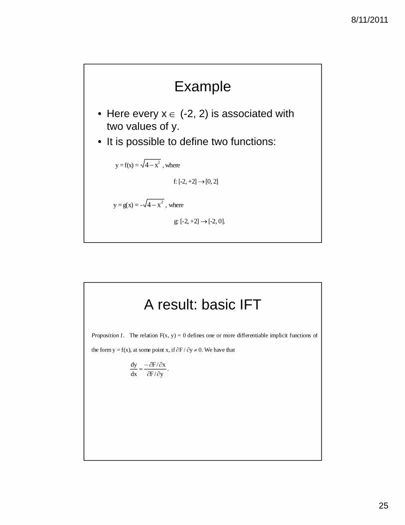
Example

• Here every x (-2, 2) is associated with t l ftwo values of y.

• It is possible to define two functions:

y = f(x) = 4 2x , where

f: [-2, +2] [0, 2] f: [ 2, 2] [0, 2]

y = g(x) = - 4 2 x , where

g: [-2, +2] [-2, 0].

A result: basic IFT

Proposition 1. The relation F(x, y) = 0 defines one or more differentiable implicit functions of

the form y = f(x), at some point x, if F / y 0. We have that

y/F

x/F

dx

dy

.

8/11/2011

26

Our Example

y =f(x) = 4 2x ; f: [-2, +2] [0, 2]y f(x) 4 x ; f: [ 2, +2] [0, 2]

y = g(x) = - 4 2x ; g: [-2, +2] [-2, 0]

f '(x) = -x(4 - x2)-1/2 = -x/y

g'(x) = +x (4 - x2)-1/2 = -x/y

Use IFT on x2 + y2 – 4 = 0.

d yd x

F xF y

xy

xy

//

,2

2

8/11/2011

27

A generalization

P 2 Th l i F( ) 0 d fi diff i bl i li iProposition 2. The relation F(x1, x2, x3, , xN) = 0 defines one or more differentiable implicit

functions of the form xi = fi(xj), at xj, if F / xi 0, i, j=1, , N, i j. We have that

i

j

j

i

x/F

x/F

x

x

.

Example

• x13 x2 + x3 x2 = 0. Find 32 / xx

x

x

F x

F x

x

x x2

3

3

2

2

13

3

/

/ ( ), for (x1

3 + x3) 0.

8/11/2011

28

A Generalized Implicit Function Theorem

• Consider a system of n equations

• The variables y1,...,yn represent n independent variables and the x1,...,xm

represent m parameters Write as y Rn

0 = Fi(y1, ...y n,x 1,... ,x m), i = 1, ...,n.

represent m parameters. Write as y Rn

and x Rm.

The Jacobian of the System

Jy =

F y F y

F y F y

n

n nn

11

1

1

/ /

/ /

y yn1/ /

8/11/2011

29

General IFT

Proposition 3. Let Fi(y,x) = 0 possess continuous partial derivatives in y and x. If at a point

i(yo,xo), |Jy| 0, then n functions yi = fi(x1,...,xm) which are defined in a neighborhood of xo. We

have

(i) Fi(f1,...fn,xo) = 0, i,

(ii) yi = fi( ) are continuously differentiable in x locally

y xk1 / F x1 / y x k1 / F x1 /

(iii) Jy

y x

y x

k

n k

1 /

/

=

F x

F x

k

nk

/

/

and

y x

y x

k

n k

1 /

/

= Jy-1

F x

F x

k

nk

/

/

.

Cramer's Rule and IFT

Remark: Using Cramer's Rule we have thatRemark: Using Cramer's Rule, we have that

yi/xk = |Jyi|/|Jy|.

8/11/2011

30

Example

Example: Solve the following system for system y1/x and y2/x.

2y1 + 3y2 - 6x = 0

y1 + 2y2 = 0.

Exponential and Logarithmic Functions

• An exponential function is a function in hi h th i d d t i blwhich the independent variable appears

as an exponent:

y = bx, where b > 1

We take b > 0 to avoid complex numbers. b > 1 is not restrictive because we canb > 1 is not restrictive because we can take (b-1)x = b-x for cases in which b (0, 1).

8/11/2011

31

Logarithmic

• A logarithmic function is the inverse f ti f bx Th t ifunction of bx. That is,

x = logby.

A preferred base is the number e 2.72. More formally, e = limn

[1 + 1/n]n. e is called the

t l l ith i b It h th d i bl t th td x x Th di lnatural logarithmic base. It has the desirable property that dx

ex= ex. The corresponding log

function is written x = ln y, meaning loge y.

Illustration

bx

y

1

x

8/11/2011

32

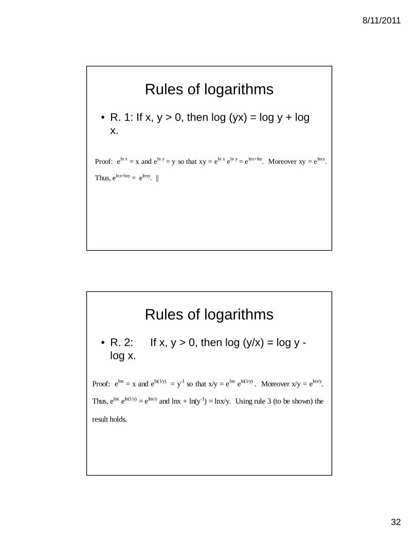
Rules of logarithms

• R. 1: If x, y > 0, then log (yx) = log y + log x.

Proof: eln x = x and eln y = y so that xy = eln x eln y = elnx+lny. Moreover xy = elnxy.

Thus, elnx+lny = elnxy. ||

Rules of logarithms

• R. 2: If x, y > 0, then log (y/x) = log y -llog x.

Proof: elnx = x and eln(1/y) = y-1 so that x/y = elnx eln(1/y) . Moreover x/y = elnx/y.

Thus, elnx eln(1/y) = elnx/y and lnx + ln(y-1) = lnx/y. Using rule 3 (to be shown) the

result holds.

8/11/2011

33

Rules of logarithms

• R. 3: If x > 0, then log xa = a log x.

Proof: elnx = x and axeln = xa. However, xa = (elnx)a = ealnx. Thus,

axeln = ealnx. ||

Conversion and inversion of bases

• conversion

logbu = (logbc)(logcu) (logcu is known)

Proof: Let u = cp. Then logc u = p. We know that logb u = logb cp = plogb c. By definition, p =

logc u, so that logb u = (logc u)(logb c). ||

8/11/2011

34

Conversion and inversion of bases

• inversion

logbc = 1/(logcb)

Proof: Using the conversion rule, 1 = logb b = (logb c)(logc b). Thus, logb c = 1/(logc b). ||

Derivatives of Exponential and Logarithmic Functions.

• R. 1: The derivative of the log function l f( ) i i by = ln f(x) is given by

d yd x

f xf x

( )( )

8/11/2011

35

Derivatives of Exponential and Logarithmic Functions

• R. 2: The derivative of the exponential f ti f(x) i i bfunction y = ef(x) is given by

dy

dx= f(x)ef(x).

Derivatives of Exponential and Logarithmic Functions

• R. 3: The derivative of the exponential f ti bf(x) i i bfunction y = bf(x) is given by

dy

dx= f(x)bf(x)ln b.

8/11/2011

36

Derivatives of Exponential and Logarithmic Functions

• R. 4: The derivative of the logarithmic f ti l f( ) i i bfunction y = logbf(x) is given by

d yd x

f xf x b

( )( ) l n

1

Examples

#1 L e t y = e x2 42 , th en y ,

d yd x

= 4x e x2 42 .

# 2 L e t y = [ l n ( 1 6 x 2 ) ] x 2

d y

d x =

3 2

1 6 2

x

xx 2 + 2 x l n ( 1 6 x 2 )

= 2 x + 2 x l n 1 6 x 2 = 2 x + 2 x ( l n 1 6 + 2 l n x )

= 2 x ( 1 + l n 1 6 ) + 4 x l n x .

8/11/2011

37

Examples

#3 Let y = 62 17x x , then f' = (2x + 17) 6

2 17x x ln 6.

The Taylor Series Approximation

• It is sometimes of interest to approximate f ti t i t ith th fa function at a point with the use of a

polynomial function.

• Linear and quadratic approximations are typically used.

• Let y = f(x)• Let y = f(x).

8/11/2011

38

The Taylor Series Approximation

• A Taylor's Series Approximation of f at xo

i i bis given by

f(x) f(xo) + .)xx(dx

)x(fd

!i

1 ioi

oik

1i

Linear Approximation

• A linear approximation takes k = 1. This is given byby

f(x) f(xo) + [df(xo)/dx](x-xo) = [f(xo) – f '(xo)xo] + f '(xo)x.

• Defining, a [f(xo) – f '(xo)xo ] and b f '(xo), we have

f(x) a + bx.

8/11/2011

39

Illustration

f(xo) A Note that A = f – (f – f 'x) and A/x = f ' [f(xo) – f ' (xo)xo] xo

Quadratic Approximation

• A quadratic approximation takes k = 2. We have thatWe have that

• or

f(x) f(xo) + f '(xo)(x-xo) + .)xx(2

)x(''f 2oo

f( ) [f( o) f '( o) o + f ''( o)( o)2/2] + [f '( o) of ''( o)] +[f ''( o)/2] 2

• This is of the form

f(x) [f(xo) – f '(xo)xo+ f ''(xo)(xo) /2] + [f '(xo) – xof ''(xo)]x + [f ''(xo)/2]x

f(x) a + bx + cx2.

8/11/2011

40

Functions of many variables

• General linear

f( x) f( xo) +

n

1i

oii

oi ).xx)(x(f

Define f(x)' (f1(x)…fn(x)) and term this the gradient of f. Then we have

f(x) f(xo) + f(xo)'(x – xo),

Functions of many variables

• Quadratic

• or

f( x ) f ( x o ) + f (x o ) '(x – x o ) +

'

) .xx)(xx)(x(f2

1 ojj

oii

o

i j i j

f ( x ) f ( x o ) + f ( x o ) '( x – x o ) + 2

1( x – x o ) 'H ( x o ) ( x - x o ) .

8/11/2011

41

Examples

Consider the function y = 2x2. Let us construct a linear approximation at x = 1.y pp

f 2 + 4(x – 1) = -2 + 4x.

A quadratic approximation at x = 1 is f 2 + 4(x – 1) + (4/2)(x-1)2 = 2 + 4x – 4 + 2(x2 –2x + 1) = 2 + 4x – 4 + 2x2 –4x + 2) f = 2x2. Given that the original function is quadratic, the approximation is exact.

Examples. Let y = x1

3x2. Construct a linear and a quadratic approximation of f at (1,1). The linear

approximation is given by

f 1 + 3(x1 – 1) + 1(x2 – 1).

Rewriting,

f -3 + 3x1 + x2.

A quadratic approximation is constructed as follows:

1 36 1x1 f 1 + 3(x1 – 1) + 1(x2 – 1) + 2

1[x1 – 1 x2 – 1]

03

36

1x

1x

2

1 .

Expanding terms we obtain the following expression.

f 3 - 6x1 - 2x2 + 3 x1x2 + 3x12.