Lecture 5: Antennas and Wave Propagation

Anders Västberg

vastberg@kth.se

08-790 44 55

Digital Communication System

Source of Information

SourceEncoder

Modulator RF-Stage

Channel

RF-StageInformation

SinkSource

DecoderDemodulator

ChannelEncoder

DigitalModulator

ChannelDecoder

DigitalDemodulator

[Slimane]

Maxwell's Equations

• Electrical field lines may either start and end on charges, or are continuous

• Magnetic field lines are continuous

• An electric field is produced by a time-varying magnetic field

• A magnetic field is produced by a time-varying electric field or by a current

Radiation

Only accelerating charges produce radiation

[Saunders, 1999]

Electromagnetic Fields

)cos(}{),( tetrE tj EE

(V/m),2

1ErmsE

HEP

H2

1rmsH

)(W/m,2

1

2

1 2HEP S

Poyntings Vector:

Power density:

Impedance of Free Space

• Both fields carry the same amount of energy

• Free space impedance is given by

• The power density can be expressed as

H/m104

F/m10854185.87

0

120

22

0

HE

3770

00

Z

20

0

2

rmsrms HZZ

ES

[Slimane]

Isotropic Antenna

• An isotropic radiator is an hypothetical antenna that generates a uniform field, i.e., energy flows with equal strength in all directions.

• Let Pt be the total power emitted by this antenna.

• This total power will be uniformly distributed over the surface of a sphere enclosing the antenna.

• The power density on a sphere of radius r is given by:

22

W/m,4 r

PS tr

[Slimane]

Effective Aperture of an Antenna

• Ae is defined as the area of a perfect lossless antenna

• The received power can be written as follows:

• Ae is dependent on the type of receiving antenna

24 r

APASP eterr

[Slimane]

Antenna Gain

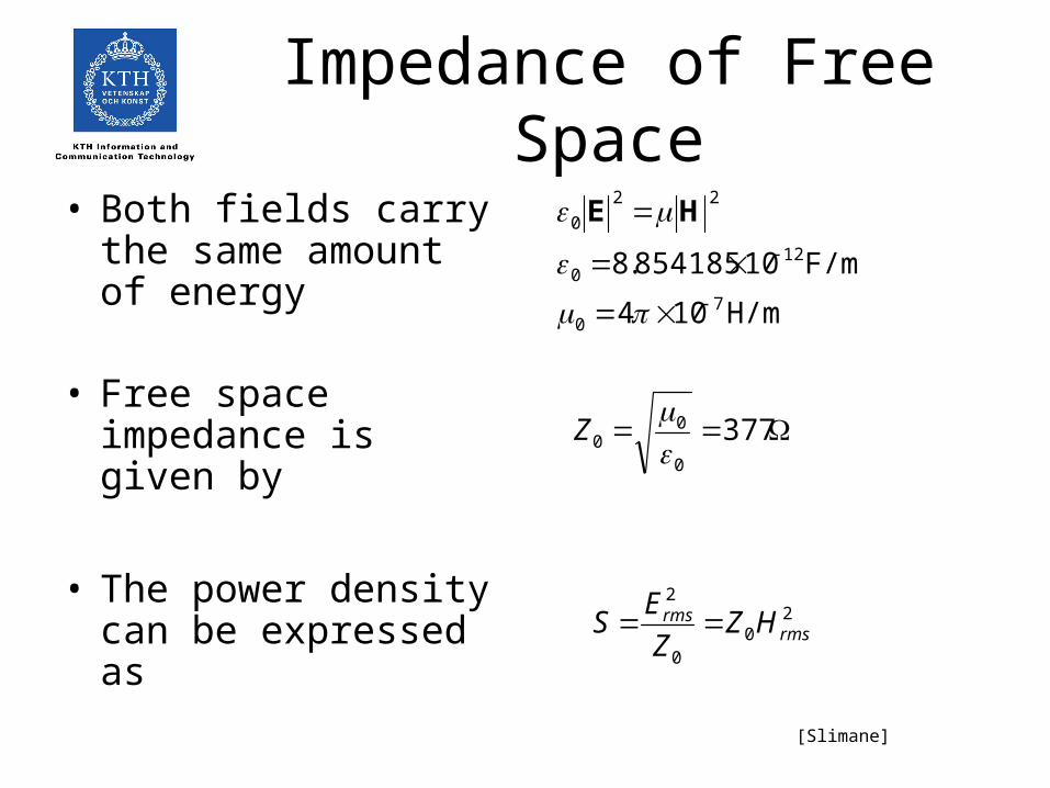
2

2

2

44

c

AfAG ee

• The antenna gain is defined by its relative power density

),(max SG

24

),(),,(

r

PS

SSrS

tr

rr

Wave propagation

• The field at the receiver can be decomposed into three components– Direct wave, Line-of-Sight Path– Ground reflected wave– Ground Wave (less than 2 MHz, less than 10 MHz over water)

[Slimane]

Plane Earth Model

[Slimane]

Plane Earth Model

[Slimane]

Diffraction

[Saunders, 1999]

Diffraction

• For radio wave propagation over rough terrain, the propagation is dependent on the size of the object encountered.

• Waves with wavelengths much shorter than the size of the object will be reflected

• Waves with wavelengths much larger than the size of the obstacle will pass virtually unaffected.

• Waves with intermediate wavelengths curve around the edges of the obstacles in their propagation (diffraction).

• Diffraction allows radio signals to propagate around the curved surface and propagate behind obstacles.

[Slimane]

Propagation in the Atmosphere

• The atmosphere around the earth contains a lot of gazes (1044 molecules)

• It is most dense at the earth surface (90% of molecules below a height of 20 km).

• It gets thinner as we reach higher and higher attitudes.

• The refractive index of the air in the atmosphere changes with the Height

• This affects the propagation of radio waves.• The straight line propagation assumption may

not be valid especially for long distances.

[Slimane]

Effective Earth Radius

[Slimane]

Microwave Communication

[Slimane]

Line-of-Sight Range

[Slimane]

Fresnel Zone

[Slimane]

Ionospheric Communication

[Davies, 1993]

Propagation Modelling

[Slimane]

Propagation Modelling

[Slimane]