Lecture 4:

• Trials and Tribula,ons! • Uncertain,es

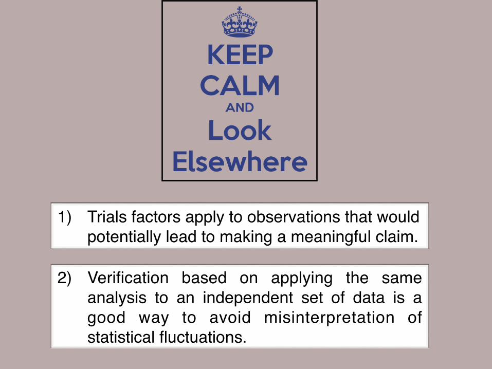
1) Trials factors apply to observations that would potentially lead to making a meaningful claim.

2) Verification based on applying the same analysis to an independent set of data is a good way to avoid misinterpretation of statistical fluctuations.

7776

Pop Quiz:100 true/false questions on details of 17th century Swedish architecture.

100 true/false questions on details of 17th century Danish architecture.

0 25 50 75 100number of correct answers

0 25 50 75 100number of correct answers

What an improvement! This particular group of students must know much more about Danish architecture!!

“Regression to the Mean”

100 75 50 25 0 0

2

5

5

0

7

5

1

00

First Test Score

Seco

nd Te

st Sc

ore

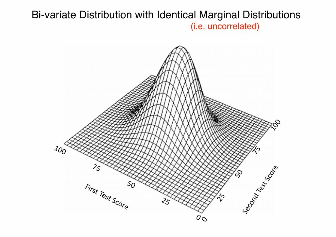
Bi-variate Distribution with Identical Marginal Distributions(i.e. uncorrelated)

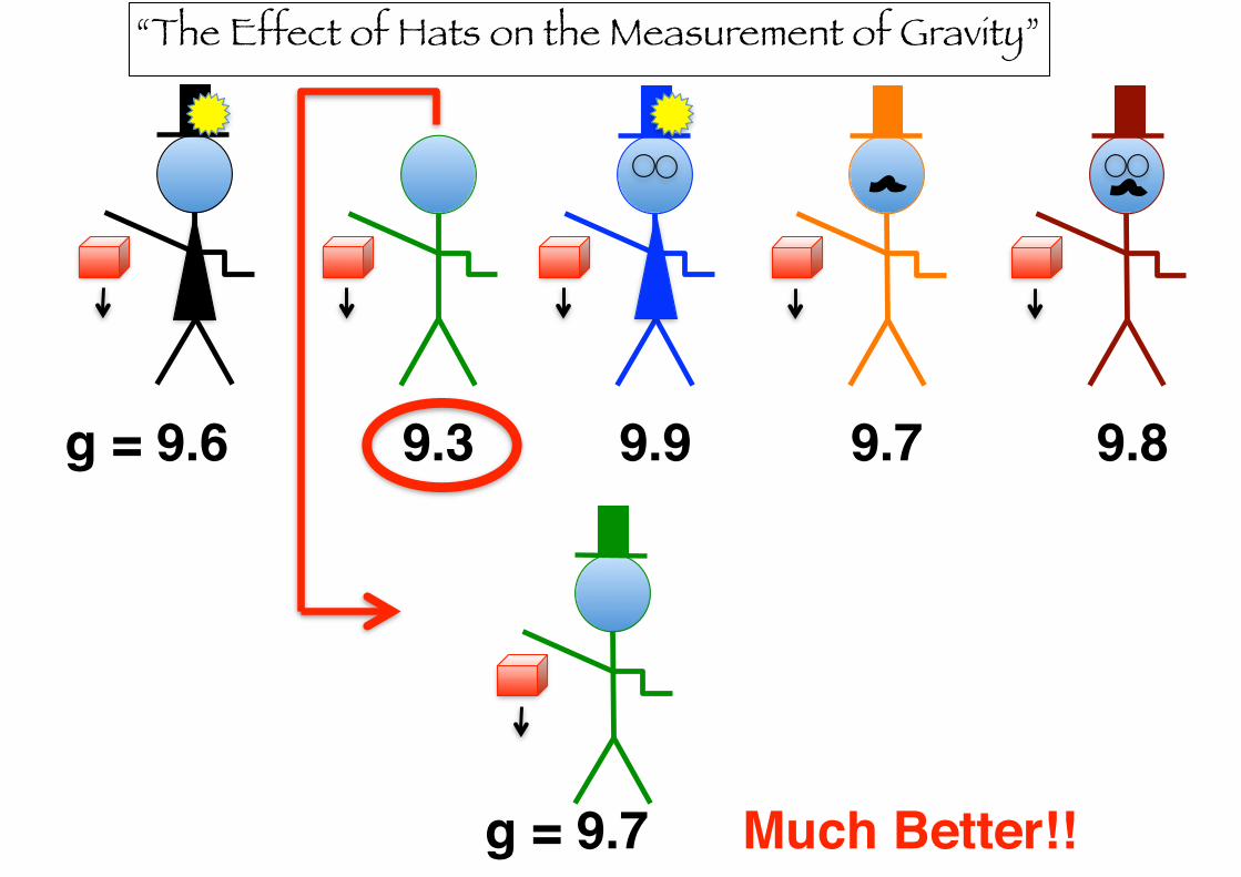
g = 9.6 9.3 9.9 9.7 9.8

“The Effect of Hats on the Measurement of Gravity”

g = 9.7 Much Better!!

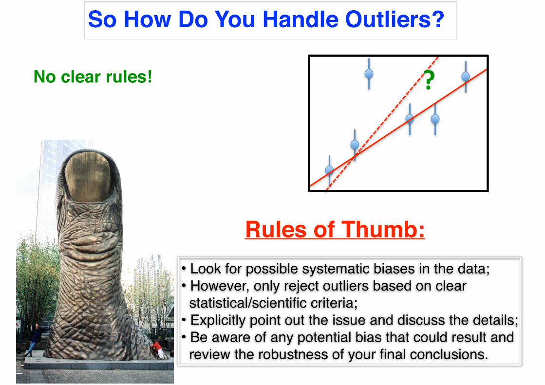
So How Do You Handle Outliers?

• Look for possible systematic biases in the data;• However, only reject outliers based on clear statistical/scientific criteria;• Explicitly point out the issue and discuss the details;• Be aware of any potential bias that could result and review the robustness of your final conclusions.

Rules of Thumb:

?No clear rules!

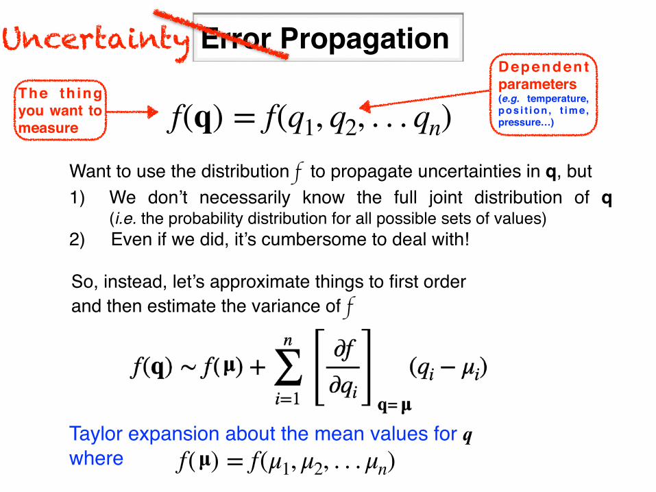
Error Propagation

Want to use the distribution f to propagate uncertainties in q, but 1) We don’t necessarily know the full joint distribution of q

(i.e. the probability distribution for all possible sets of values)2) Even if we did, it’s cumbersome to deal with!

So, instead, let’s approximate things to first orderand then estimate the variance of f

Uncertainty

f(q) = f(q1, q2, . . . qn)

Taylor expansion about the mean values for qwhere f(μ) = f(μ1, μ2, . . . μn)µ

The th ing you want to measure

Dependent parameters (e.g. temperature, p o s i t i o n , t i m e , pressure…)

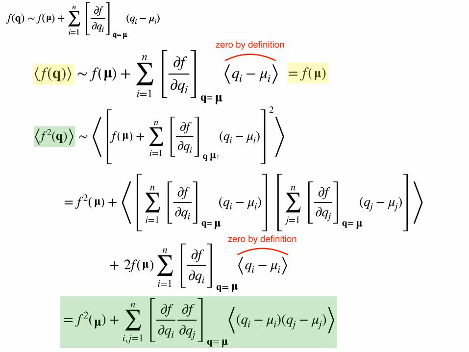
zero by definition

zero by definition

= f(μ)µ⟨ f(q)⟩ ∼ f(μ) +n

∑i=1 [ ∂f

∂qi ]q=μ

⟨qi − μi⟩µµ

⟨f 2(q)⟩ ∼ ⟨ f (μ) +n

∑i=1 [ ∂f

∂qi ]q=μ

(qi − μi)

2

⟩µ

µ

= f 2(μ) + ⟨n

∑i=1 [ ∂f

∂qi ]q=μ

(qi − μi)n

∑j=1 [ ∂f

∂qj ]q=μ

(qj − μj) ⟩µ

µ µ

+ 2f(μ)n

∑i=1 [ ∂f

∂qi ]q=μ

⟨qi − μi⟩µ

µ

= f 2(μ) +n

∑i, j=1 [ ∂f

∂qi

∂f∂qj ]q=μ

⟨(qi − μi)(qj − μj)⟩µµ

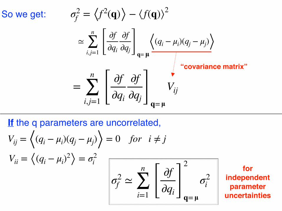
So we get: σ2f = ⟨f 2(q)⟩ − ⟨ f(q)⟩2

≃n

∑i, j=1 [ ∂f

∂qi

∂f∂qj ]q=μ

⟨(qi − μi)(qj − μj)⟩µ

Vij = ⟨(qi − μi)(qj − μj)⟩ = 0 for i ≠ j

Vii = ⟨(qi − μi)2⟩ = σ2i

σ2f ≃

n

∑i=1 [ ∂f

∂qi ]2

q=μ

σ2i

µ

for independent parameter

uncertainties

If the q parameters are uncorrelated,

=n

∑i,j=1 [ ∂f

∂qi

∂f∂qj ]q=μ

Vijµ

“covariance matrix”

Some simple examples:

Ttot = t1 + t2

σ2T ≃ [ ∂T

∂t1 ]2

σ21 + [ ∂T

∂t2 ]2

σ22

σ2s ≃ [ ∂s

∂v ]2

σ2v + [ ∂s

∂t ]2

σ2t

= σ21 + σ2

2

= t2σ2v + v2σ2

t

( σs

s )2

≃ ( σv

v )2

+ ( σt

t )2

s = vt

For a quadrature addi,on of uncertain,es, uncertain,es that are half as big only carry 1/4 of the weight, and uncertain,es that are 1/4 as big only carry 1/16 of the weight... Only the dominant uncertain5es ma7er!

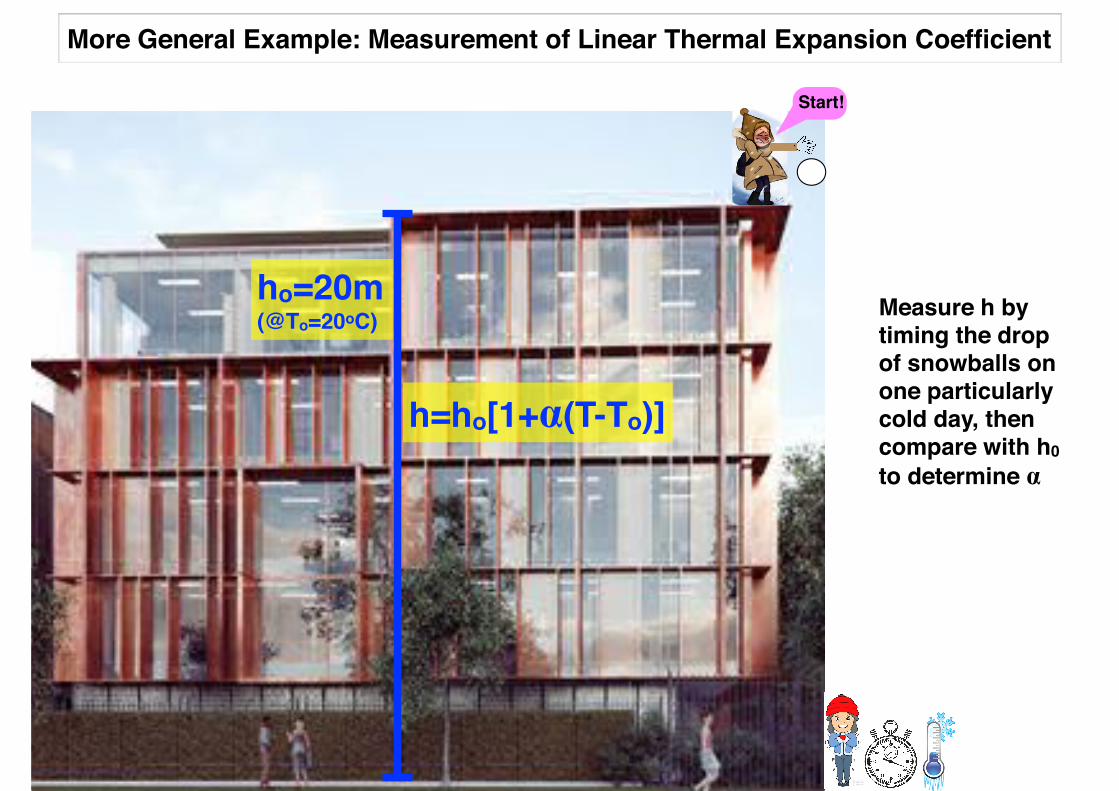
ho=20m(@To=20oC)

h=ho[1+α(T-To)]

More General Example: Measurement of Linear Thermal Expansion Coefficient

Start!

Measure h by timing the drop of snowballs on one particularly cold day, then compare with h0 to determine α

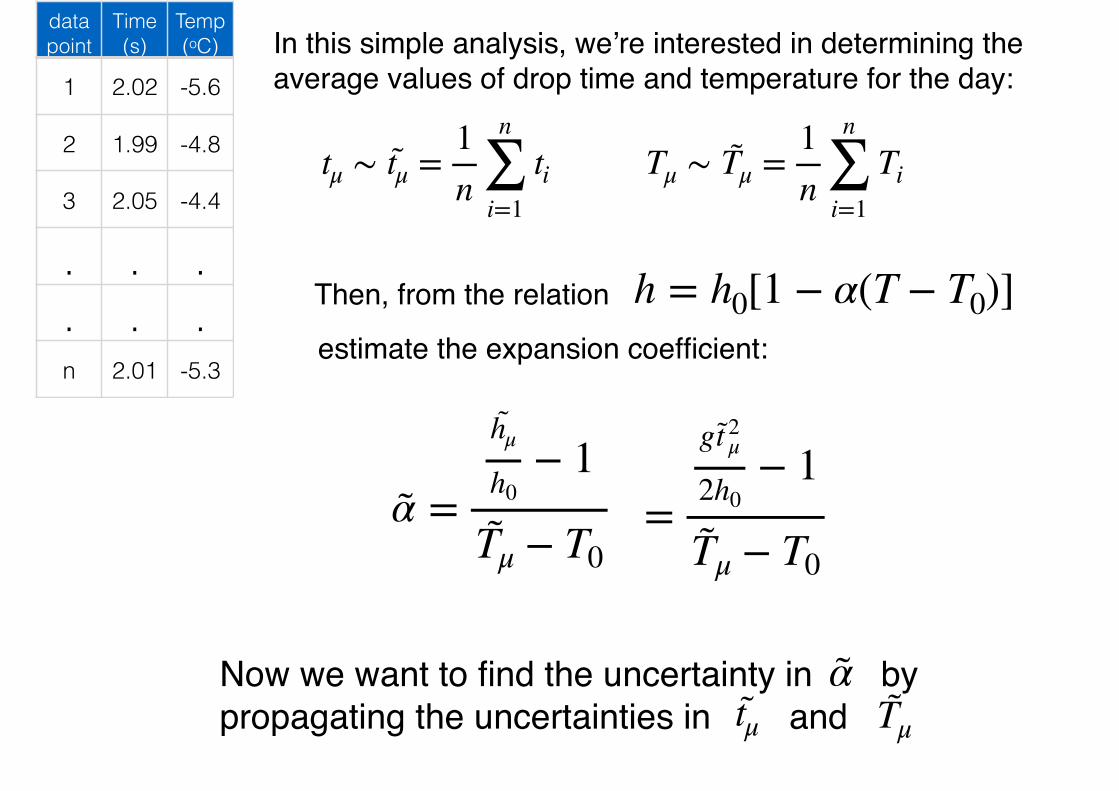
data point

Time (s)

Temp (oC)

1 2.02 -5.6

2 1.99 -4.8

3 2.05 -4.4

. . .

. . .n 2.01 -5.3

tμ ∼ t̃μ = 1n

n

∑i=1

ti Tμ ∼ T̃μ = 1n

n

∑i=1

Ti

In this simple analysis, we’re interested in determining the average values of drop time and temperature for the day:

h = h0[1 − α(T − T0)]Then, from the relation

estimate the expansion coefficient:

α̃ =h̃μ

h0− 1

T̃μ − T0=

gt̃ 2μ

2h0− 1

T̃μ − T0

Now we want to find the uncertainty in by propagating the uncertainties in and

α̃t̃μ T̃μ

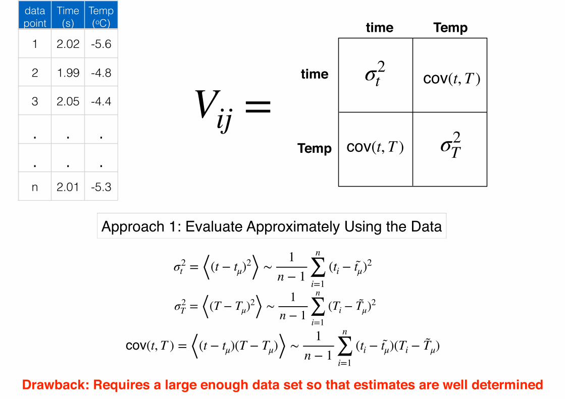
data point

Time (s)

Temp (oC)

1 2.02 -5.6

2 1.99 -4.8

3 2.05 -4.4

. . .

. . .n 2.01 -5.3

Approach 1: Evaluate Approximately Using the Data

σ2t = ⟨(t − tμ)2⟩ ∼ 1

n − 1n

∑i=1

(ti − t̃μ)2

σ2T = ⟨(T − Tμ)2⟩ ∼ 1

n − 1n

∑i=1

(Ti − T̃μ)2

cov(t, T ) = ⟨(t − tμ)(T − Tμ)⟩ ∼ 1n − 1

n

∑i=1

(ti − t̃μ)(Ti − T̃μ)

Drawback: Requires a large enough data set so that estimates are well determined

Vij =

time

time

Temp

Temp

σ2t

σ2T

cov(t, T )

cov(t, T )

Vij =

time

time

Temp

Temp

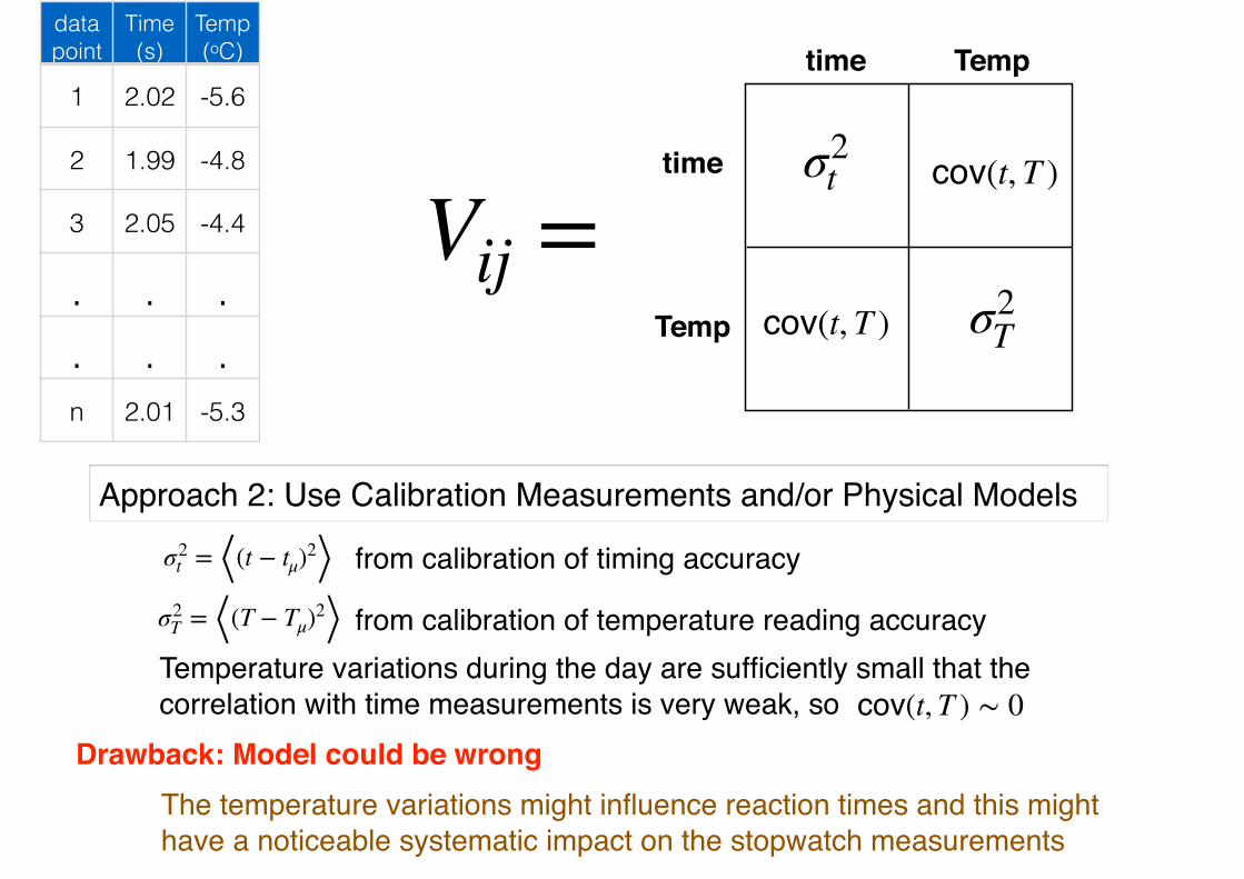
Approach 2: Use Calibration Measurements and/or Physical Models

Drawback: Model could be wrong

σ2t = ⟨(t − tμ)2⟩ from calibration of timing accuracy

σ2T = ⟨(T − Tμ)2⟩ from calibration of temperature reading accuracy

Temperature variations during the day are sufficiently small that the correlation with time measurements is very weak, so cov(t, T ) ∼ 0

data point

Time (s)

Temp (oC)

1 2.02 -5.6

2 1.99 -4.8

3 2.05 -4.4

. . .

. . .n 2.01 -5.3

The temperature variations might influence reaction times and this might have a noticeable systematic impact on the stopwatch measurements

σ2t

σ2T

cov(t, T )

cov(t, T )

Vij =

time

time

Temp

Temp

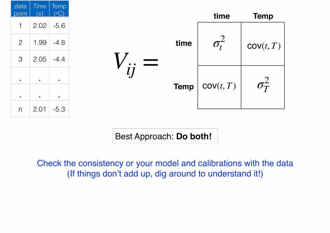
Best Approach: Do both!

Check the consistency or your model and calibrations with the data(If things don’t add up, dig around to understand it!)

data point

Time (s)

Temp (oC)

1 2.02 -5.6

2 1.99 -4.8

3 2.05 -4.4

. . .

. . .n 2.01 -5.3

σ2t

σ2T

cov(t, T )

cov(t, T )

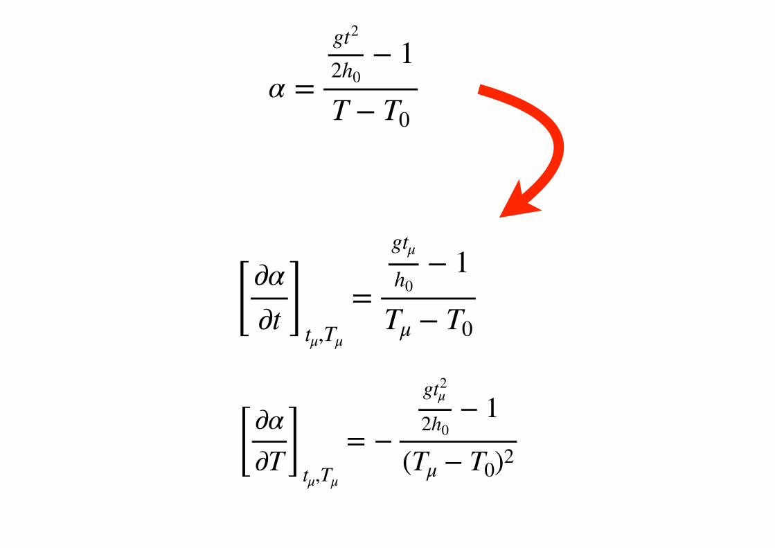
α =gt2

2h0− 1

T − T0

[ ∂α∂t ]

tμ,Tμ

=gtμh0

− 1Tμ − T0

[ ∂α∂T ]

tμ,Tμ

= −gt2

μ

2h0− 1

(Tμ − T0)2

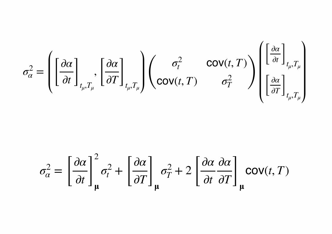
σ2α = [ ∂α

∂t ]tμ,Tμ

, [ ∂α∂T ]

tμ,Tμ( σ2

t cov(t, T )cov(t, T ) σ2

T )[ ∂α

∂t ]tμ,Tμ

[ ∂α∂T ]tμ,Tμ

σ2α = [ ∂α

∂t ]2

μσ2

t + [ ∂α∂T ]

μσ2

T + 2 [ ∂α∂t

∂α∂T ]

μcov(t, T )

µµ µ

Typical linear expansion coefficients for building materials ~5x10-6 per oC

Take (T-To) ~ 20oC

h0-h ~ (20m)(5x10-6)(20oC) = 0.002m

velocity at impact = 2gh0 = 2(9.8m /s2)(20m) ∼ 20m /sSo, timing must be known to an accuracy of (0.002/20) = 0.0001s

Accuracy of any one timing timing measurement ~ 0.1s

But we improve by averaging lots of measurements according to σm = σn

How many measurements do we need?

n = σ2

σ2m∼ ( 0.1

0.0001 )2

= 106 (ignoring systematic uncertainties!)

The Statistical Calculation That You Should Have Done at the Start!

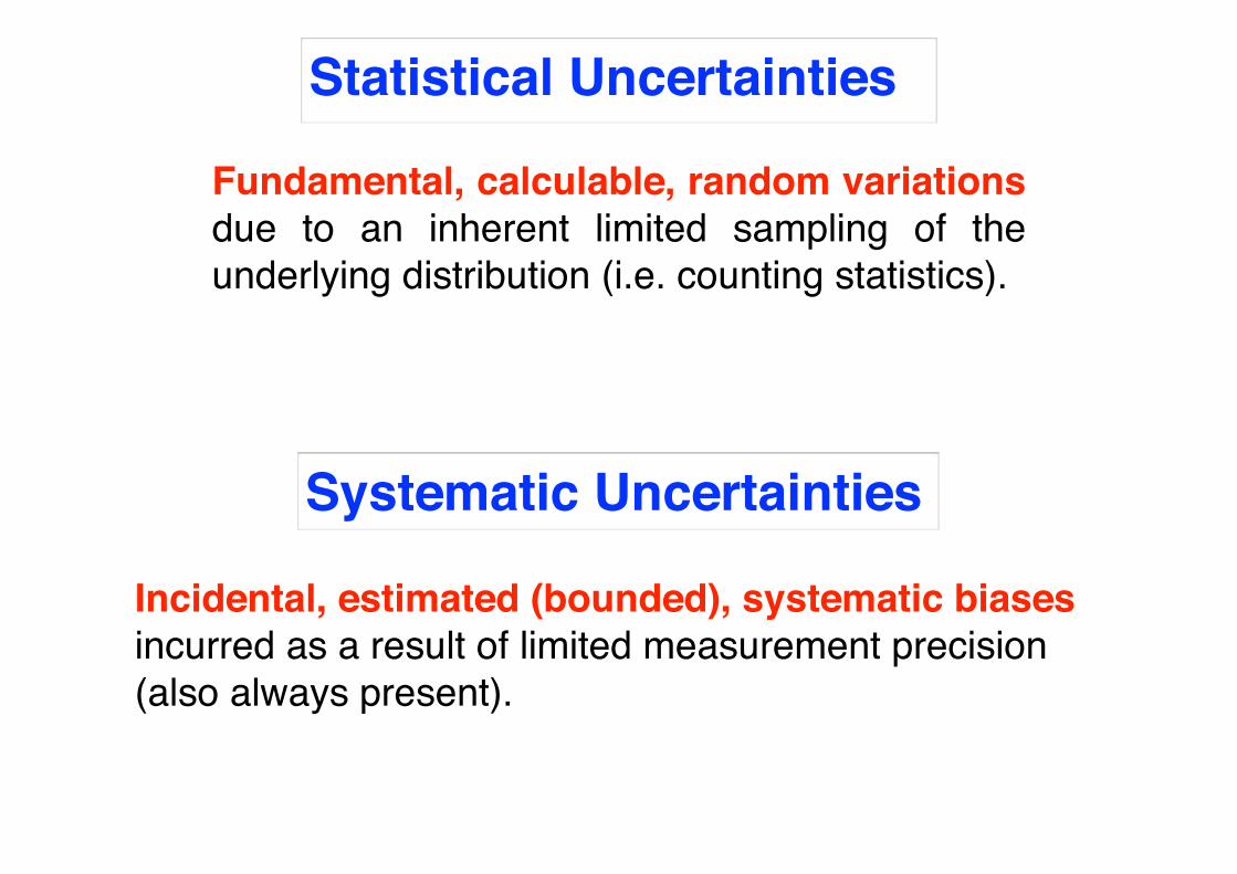
Statistical Uncertainties

Fundamental, calculable, random variations due to an inherent limited sampling of the underlying distribution (i.e. counting statistics).

Systematic Uncertainties

Incidental, estimated (bounded), systematic biasesincurred as a result of limited measurement precision(also always present).

There is no universally applicable method for estimating/bounding* systematic uncertainties. A typical approach often relies on independent cross-checks, accounting for possible statistical limitations of calibration procedures, knowledge about the experimental design and general consistency arguments.

* Systematic errors that are “determined” become corrections!

Because of their very different nature, there is no standard, mathematically rigorous way to combine the 2 types of uncertainties. The convention is thus to quote results in the form:

Result ± Uncertainty (stat) ± Uncertainty (sys)

And error bars such as: or sysquadraturesum of sysand stat

or sysquadraturesum of sysand stat

How do you then make use of such data points to fit a model?

It is often generally assumed that systematic uncertainties can be treated in a similar way to statistical uncertainties, with careful attention to correlations.

Ideally, the best way to treat systematic uncertainties are as free parameters in the model fit, constrained by the separately determined bounds on their values.