Lecture 4. Logistic Regression. Basis Expansion · Statistical Machine Learning (S2 2017) Deck 4 Logistic regression model 6-10 -5 0 5 10 0.0 0.2 0.4 0.6 0.8 1.0 Logistic function

Semester 2, 2017Lecturer: Andrey Kan

Lecture 4. Logistic Regression. Basis Expansion

COMP90051 Statistical Machine Learning

Copyright: University of Melbourne

Statistical Machine Learning (S2 2017) Deck 4

This lecture

• Logistic regression∗ Binary classification problem∗ Logistic regression model

• Basis expansion∗ Examples for linear and logistic regression∗ Theoretical notes

2


Logistic Regression Model

A linear method for binary classification

3


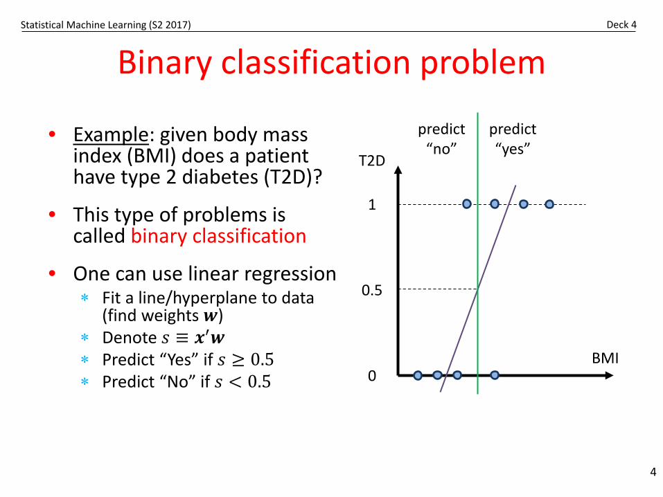
Binary classification problem

• Example: given body mass index (BMI) does a patient have type 2 diabetes (T2D)?

• This type of problems is called binary classification

• One can use linear regression∗ Fit a line/hyperplane to data

(find weights 𝒘𝒘)∗ Denote 𝑠𝑠 ≡ 𝒙𝒙′𝒘𝒘∗ Predict “Yes” if 𝑠𝑠 ≥ 0.5∗ Predict “No” if 𝑠𝑠 < 0.5

4

1

0

T2D

BMI

0.5

predict “yes”

predict “no”


Approaches to classification

• This approach can be susceptible to outliers

• Overall, the least squares criterion looks unnatural in this setting

• There are many methods developed specifically with binary classification in mind

• Examples include logistic regression, perceptron, support vector machines (SVM)

5

1

0

T2D

BMI

Confidence predictions are

penalised


Logistic regression model

6

-10 -5 0 5 10

0.0

0.2

0.4

0.6

0.8

1.0

Logistic function

RealsPr

obab

ilitie

s𝑠𝑠

𝑓𝑓𝑠𝑠

• Probabilistic approach to classification∗ 𝑃𝑃 𝒴𝒴 = 1|𝒙𝒙 = 𝑓𝑓 𝒙𝒙 = ?∗ Use a linear function? E.g., 𝑠𝑠 𝒙𝒙 = 𝒙𝒙′𝒘𝒘

• Problem: the probability needs to be between 0 and 1. Need to squash the function

• Logistic function 𝑓𝑓 𝑠𝑠 = 11+exp −𝑠𝑠

• Logistic regression model

𝑃𝑃 𝒴𝒴 = 1|𝒙𝒙 =1

1 + exp −𝒙𝒙′𝒘𝒘

• Equivalent to linear model for log-odds

log𝑃𝑃 𝒴𝒴 = 1|𝒙𝒙𝑃𝑃 𝒴𝒴 = 0|𝒙𝒙

=𝒙𝒙′𝒘𝒘


Logistic regression model

7

1

0

T2D

BMI

0.5

predict “yes”

predict “no”

• Probabilistic approach to classification∗ 𝑃𝑃 𝒴𝒴 = 1|𝒙𝒙 = 𝑓𝑓 𝒙𝒙 = ?∗ Use a linear function? E.g., 𝑠𝑠 𝒙𝒙 = 𝒙𝒙′𝒘𝒘

• Problem: the probability needs to be between 0 and 1. Need to squash the function

• Logistic function 𝑓𝑓 𝑠𝑠 = 11+exp −𝑠𝑠

• Logistic regression model

𝑃𝑃 𝒴𝒴 = 1|𝒙𝒙 =1


• Equivalent to linear model for log-odds

log𝑃𝑃 𝒴𝒴 = 1|𝒙𝒙𝑃𝑃 𝒴𝒴 = 0|𝒙𝒙

=𝒙𝒙′𝒘𝒘

Note: here we do not use sum

of squared errors for fitting


Effect of parameter vector (2D problem)

• Decision boundary is the line where 𝑃𝑃 𝒴𝒴 = 1|𝒙𝒙 = 0.5∗ In higher dimensional problems, the decision boundary is a plane or hyperplane

• Vector 𝒘𝒘 is perpendicular to the decision boundary∗ That is, 𝒘𝒘 is a normal to the decision boundary∗ Note: in this illustration we assume 𝑤𝑤0 = 0 for simplicity

8

Murphy, Fig 8.1, p246


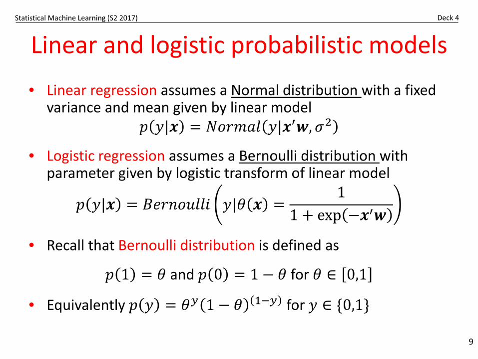
Linear and logistic probabilistic models• Linear regression assumes a Normal distribution with a fixed

variance and mean given by linear model𝑝𝑝 𝑦𝑦|𝒙𝒙 = 𝑁𝑁𝑁𝑁𝑁𝑁𝑁𝑁𝑁𝑁𝑁𝑁 𝑦𝑦|𝒙𝒙′𝒘𝒘,𝜎𝜎2

• Logistic regression assumes a Bernoulli distribution with parameter given by logistic transform of linear model

𝑝𝑝 𝑦𝑦|𝒙𝒙 = 𝐵𝐵𝐵𝐵𝑁𝑁𝐵𝐵𝑁𝑁𝐵𝐵𝑁𝑁𝑁𝑁𝐵𝐵 𝑦𝑦|𝜃𝜃 𝒙𝒙 =1


• Recall that Bernoulli distribution is defined as

𝑝𝑝 1 = 𝜃𝜃 and 𝑝𝑝 0 = 1 − 𝜃𝜃 for 𝜃𝜃 ∈ 0,1

• Equivalently 𝑝𝑝 𝑦𝑦 = 𝜃𝜃𝑦𝑦 1 − 𝜃𝜃 1−𝑦𝑦 for 𝑦𝑦 ∈ {0,1}

9


Training as maximising likelihood estimation

• Assuming independence, probability of data

𝑝𝑝 𝑦𝑦1, … ,𝑦𝑦𝑛𝑛|𝒙𝒙1, … ,𝒙𝒙𝑛𝑛 = �𝑖𝑖=1

𝑛𝑛

𝑝𝑝 𝑦𝑦𝑖𝑖|𝒙𝒙𝒊𝒊

• Assuming Bernoulli distribution we have

𝑝𝑝 𝑦𝑦𝑖𝑖|𝒙𝒙𝑖𝑖 = 𝜃𝜃 𝒙𝒙𝑖𝑖 𝑦𝑦𝑖𝑖 1 − 𝜃𝜃 𝒙𝒙𝑖𝑖1−𝑦𝑦𝑖𝑖

where 𝜃𝜃 𝒙𝒙𝑖𝑖 = 11+exp −𝒙𝒙𝑖𝑖′𝒘𝒘

• “Training” amounts to maximising this expression with respect to weights 𝒘𝒘

10


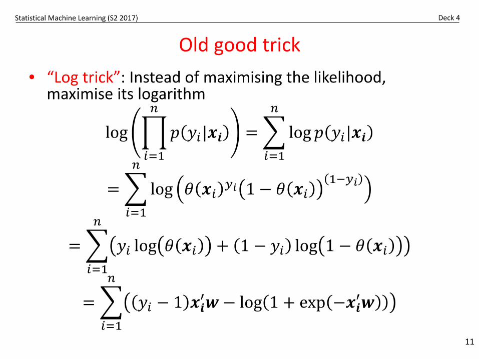
Old good trick• “Log trick”: Instead of maximising the likelihood,

maximise its logarithm

log �𝑖𝑖=1

𝑛𝑛

𝑝𝑝 𝑦𝑦𝑖𝑖|𝒙𝒙𝒊𝒊 = �𝑖𝑖=1

𝑛𝑛

log𝑝𝑝 𝑦𝑦𝑖𝑖|𝒙𝒙𝒊𝒊

= �𝑖𝑖=1

𝑛𝑛

log 𝜃𝜃 𝒙𝒙𝑖𝑖 𝑦𝑦𝑖𝑖 1 − 𝜃𝜃 𝒙𝒙𝑖𝑖1−𝑦𝑦𝑖𝑖

= �𝑖𝑖=1

𝑛𝑛

𝑦𝑦𝑖𝑖 log 𝜃𝜃 𝒙𝒙𝑖𝑖 + 1 − 𝑦𝑦𝑖𝑖 log 1 − 𝜃𝜃 𝒙𝒙𝑖𝑖

= �𝑖𝑖=1

𝑛𝑛

𝑦𝑦𝑖𝑖 − 1 𝒙𝒙𝒊𝒊′𝒘𝒘 − log 1 + exp −𝒙𝒙𝒊𝒊′𝒘𝒘

11


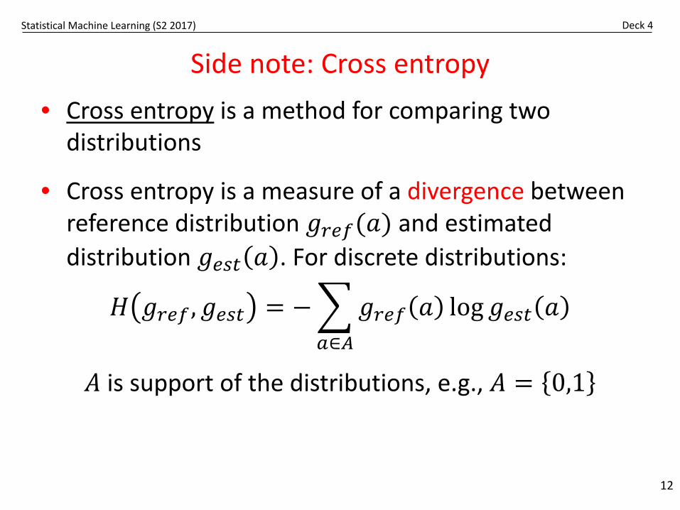
Side note: Cross entropy• Cross entropy is a method for comparing two

distributions

• Cross entropy is a measure of a divergence between reference distribution 𝑔𝑔𝑟𝑟𝑟𝑟𝑟𝑟(𝑁𝑁) and estimated distribution 𝑔𝑔𝑟𝑟𝑠𝑠𝑒𝑒 𝑁𝑁 . For discrete distributions:

𝐻𝐻 𝑔𝑔𝑟𝑟𝑟𝑟𝑟𝑟 ,𝑔𝑔𝑟𝑟𝑠𝑠𝑒𝑒 = −�𝑎𝑎∈𝐴𝐴

𝑔𝑔𝑟𝑟𝑟𝑟𝑟𝑟 𝑁𝑁 log𝑔𝑔𝑟𝑟𝑠𝑠𝑒𝑒 𝑁𝑁

𝐴𝐴 is support of the distributions, e.g., 𝐴𝐴 = 0,1

12


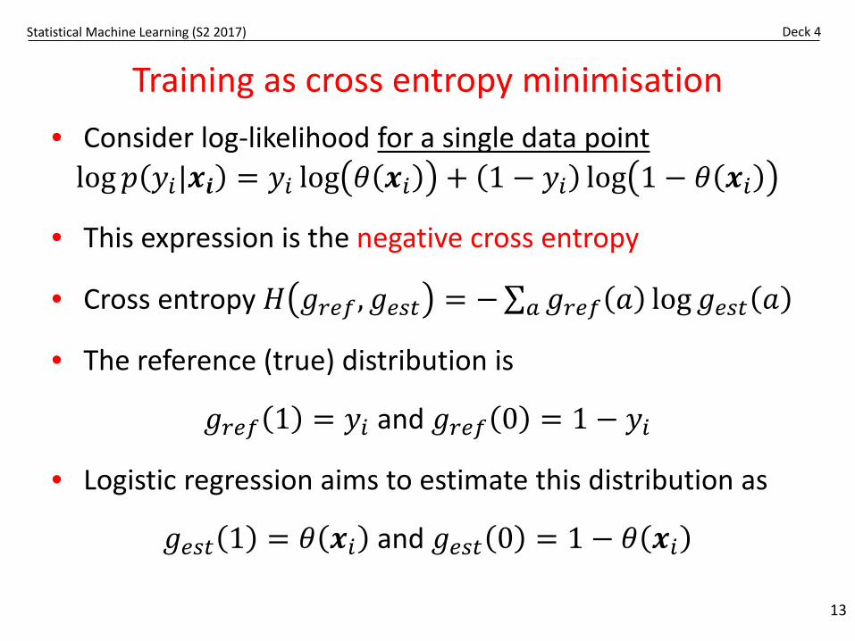
Training as cross entropy minimisation• Consider log-likelihood for a single data point

log𝑝𝑝 𝑦𝑦𝑖𝑖|𝒙𝒙𝒊𝒊 = 𝑦𝑦𝑖𝑖 log 𝜃𝜃 𝒙𝒙𝑖𝑖 + 1 − 𝑦𝑦𝑖𝑖 log 1 − 𝜃𝜃 𝒙𝒙𝑖𝑖

• This expression is the negative cross entropy

• Cross entropy 𝐻𝐻 𝑔𝑔𝑟𝑟𝑟𝑟𝑟𝑟,𝑔𝑔𝑟𝑟𝑠𝑠𝑒𝑒 = −∑𝑎𝑎 𝑔𝑔𝑟𝑟𝑟𝑟𝑟𝑟 𝑁𝑁 log𝑔𝑔𝑟𝑟𝑠𝑠𝑒𝑒 𝑁𝑁

• The reference (true) distribution is

𝑔𝑔𝑟𝑟𝑟𝑟𝑟𝑟 1 = 𝑦𝑦𝑖𝑖 and 𝑔𝑔𝑟𝑟𝑟𝑟𝑟𝑟 0 = 1 − 𝑦𝑦𝑖𝑖

• Logistic regression aims to estimate this distribution as

𝑔𝑔𝑟𝑟𝑠𝑠𝑒𝑒 1 = 𝜃𝜃 𝒙𝒙𝑖𝑖 and 𝑔𝑔𝑟𝑟𝑠𝑠𝑒𝑒 0 = 1 − 𝜃𝜃 𝒙𝒙𝑖𝑖

13


Notes on optimisation• Training logistic regression amounts to

finding 𝒘𝒘 that maximise log-likelihood∗ Equivalently, finding 𝒘𝒘 that minimise the sum of

cross entropies for each training point

• The usual routine is to set derivatives of the objective function to zero and solve

• Bad news: There is no closed form solution, iterative methods are used instead (e.g., stochastic gradient descent)

• Good news: The problem is strictly convex (like a bowl) if there are no irrelevant features

• With irrelevant features, the problem is convex (like a ridge). Regularisation methods can be applied

14

Murphy, Fig 8.3, p247𝑤𝑤1

𝑤𝑤2


Basis Expansion

Extending the utility of models via data transformation

15


Basis expansion for linear regression• Let’s take a step back. Back to linear

regression and least squares

• Real data is likely to be non-linear

• What if we still wanted to use a linear regression?∗ It’s simple, easier to understand,

computationally efficient, etc.

• How to marry non-linear data to a linear method?

16

𝑦𝑦

𝑥𝑥

• if the mountain won't come to Muhammad then Muhammad must go to the mountain

art: OpenClipartVectors at pixabay.com (CC0)


Transform the data• The trick is to transform the data: Map the data onto

another features space, such that the data is linear in that space

• Denote this transformation 𝜑𝜑:ℝ𝑚𝑚 → ℝ𝑘𝑘. If 𝒙𝒙 is the original set of features 𝜑𝜑 𝒙𝒙 denotes the new set of features

• Example: suppose there is just one feature 𝑥𝑥, and the data is scattered around a parabola rather than a straight line

17

𝑦𝑦

𝑥𝑥


Example: Polynomial regression• No worries, just define

𝜑𝜑1 𝑥𝑥 = 𝑥𝑥𝜑𝜑2 𝑥𝑥 = 𝑥𝑥2

• Next, apply linear regression to 𝜑𝜑1,𝜑𝜑2𝑦𝑦 = 𝑤𝑤0 + 𝑤𝑤1𝜑𝜑1 𝑥𝑥 + 𝑤𝑤2𝜑𝜑2 𝑥𝑥 = 𝑤𝑤0 + 𝑤𝑤1𝑥𝑥 + 𝑤𝑤2𝑥𝑥2

and here you have quadratic regression

• More generally, obtain polynomial regression if the new set of attributes are powers of 𝑥𝑥

18

𝑦𝑦

𝑥𝑥


Basis expansion• Data transformation, also known as basis expansion, is a

general technique∗ We’ll see more examples throughout the course

• It can be applied for both regression and classification

• There are many possible choices of 𝜑𝜑

19

φ


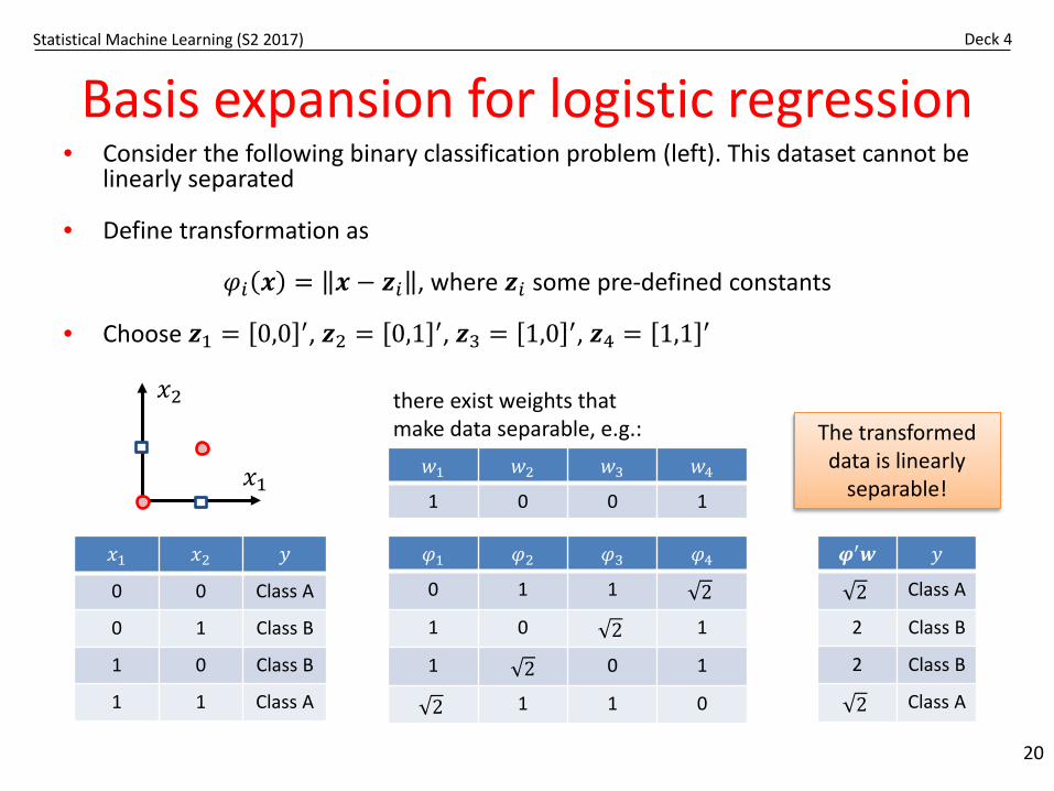
Basis expansion for logistic regression• Consider the following binary classification problem (left). This dataset cannot be

linearly separated

• Define transformation as

𝜑𝜑𝑖𝑖 𝒙𝒙 = 𝒙𝒙 − 𝒛𝒛𝑖𝑖 , where 𝒛𝒛𝑖𝑖 some pre-defined constants

• Choose 𝒛𝒛1 = 0,0 ′, 𝒛𝒛2 = 0,1 ′, 𝒛𝒛3 = 1,0 ′, 𝒛𝒛4 = 1,1 ′

20

𝑥𝑥1 𝑥𝑥2 𝑦𝑦

0 0 Class A

0 1 Class B

1 0 Class B

1 1 Class A

𝑥𝑥1

𝑥𝑥2

𝜑𝜑1 𝜑𝜑2 𝜑𝜑3 𝜑𝜑40 1 1 2

1 0 2 1

1 2 0 1

2 1 1 0

𝑤𝑤1 𝑤𝑤2 𝑤𝑤3 𝑤𝑤41 0 0 1

𝝋𝝋′𝒘𝒘 𝑦𝑦

2 Class A

2 Class B

2 Class B

2 Class A

The transformed data is linearly

separable!

there exist weights that make data separable, e.g.:


Radial basis functions• The above transformation is an example of the use of

radial basis functions (RBFs)∗ Their use has been motivated from the approximation

theory, where sums of RBFs are used to approximate given functions

• A radial basis function is a function of the form 𝜑𝜑 𝒙𝒙 = 𝜓𝜓 𝒙𝒙 − 𝒛𝒛 , where 𝒛𝒛 is a constant

• Examples:

• 𝜑𝜑 𝒙𝒙 = 𝒙𝒙 − 𝒛𝒛

• 𝜑𝜑 𝒙𝒙 = exp − 1𝜎𝜎𝒙𝒙 − 𝒛𝒛 2

21

𝜑𝜑 𝑥𝑥

𝑥𝑥


Challenges of basis expansion• Basis expansion can significantly increase the utility of

methods, especially, linear methods

• In the above examples, one limitation is that the transformation needs to be defined beforehand∗ Need to choose the size of the new feature set∗ If using RBFs, need to choose 𝒛𝒛𝑖𝑖

• Regarding 𝒛𝒛𝑖𝑖, one can choose uniformly space points, or cluster training data and use cluster centroids

• Another popular idea is to use training data 𝒛𝒛𝑖𝑖 ≡ 𝒙𝒙𝑖𝑖∗ E.g., 𝜑𝜑𝑖𝑖 𝒙𝒙 = 𝜓𝜓 𝒙𝒙 − 𝒙𝒙𝑖𝑖∗ However, for large datasets, this results in a large number of

features computational hurdle

22


Further directions• There are several avenues for taking the idea of basis

expansion to the next level∗ Will be covered later in this subject

• One idea is to learn the transformation 𝜑𝜑 from data∗ E.g., Artificial Neural Networks

• Another powerful extension is the use of the kernel trick∗ “Kernelised” methods, e.g., kernelised perceptron

• Finally, in sparse kernel machines, training depends only on a few data points∗ E.g., SVM

23


This lecture

• Logistic regression∗ Binary classification problem∗ Logistic regression model

• Basis expansion∗ Examples for linear and logistic regression∗ Theoretical notes

24

Documents

Lecture 4. Logistic Regression. Basis Expansion · Statistical Machine Learning (S2 2017) Deck 4 Logistic regression model 6-10 -5 0 5 10 0.0 0.2 0.4 0.6 0.8 1.0 Logistic function