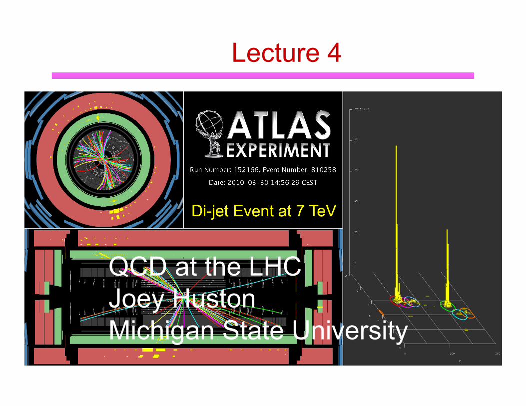
Lecture 4

QCD at the LHC Joey Huston Michigan State University

A question from Eric   Why do the low number eigenvectors correspond to the

best determined directions?   These are the directions in which the χ2 function

increases most steeply if you vary the parameters from the their central fit values

 Finishing up on PDFs

My recommendation to PDF4LHC/Higgs working group

  Cross sections should be calculated with MSTW2008, CTEQ6.6 and NNPDF

  Upper range of prediction should be given by upper limit of error prediction using prescription for combining αs uncertainty with error PDFs ◆  in quadrature for CTEQ6.6 and NNPDF ◆  using eigenvector sets for different values of αs for MSTW2008 ◆  (my suggestion) as standard, use 90%CL limits ◆  note that this effectively creates a larger αs uncertainty range

  Ditto for lower limit   So for a Higgs mass of 120 GeV at 14 TeV,it turns out that the gg cross

section lower limit would be defined by the CTEQ6.6 lower limit (PDF+αs error) and the upper limit defined by the MSTW2008 upper limit (PDF+αs error) ◆  with the difference between the central values primarily due to αs

◆  I’ll come back to using the Higgs as an example in the last lecture   To fully understand similarities/differences of cross sections/uncertainties

conduct a benchmarking exercise, to which all groups are invited to participate

  To be discussed in lecture #5

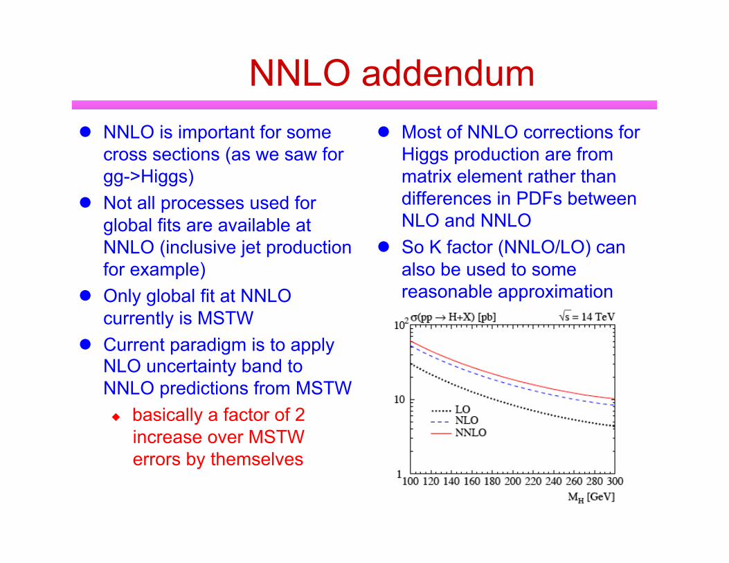
NNLO addendum   NNLO is important for some

cross sections (as we saw for gg->Higgs)

  Not all processes used for global fits are available at NNLO (inclusive jet production for example)

  Only global fit at NNLO currently is MSTW

  Current paradigm is to apply NLO uncertainty band to NNLO predictions from MSTW ◆  basically a factor of 2

increase over MSTW errors by themselves

  Most of NNLO corrections for Higgs production are from matrix element rather than differences in PDFs between NLO and NNLO

  So K factor (NNLO/LO) can also be used to some reasonable approximation

For CTEQ: αs series   Take CTEQ6.6 as base, and vary

αs(mZ) +/-0.002 (in 0.001 steps) around central value of 0.118

  Blue is the PDF uncertainty from eigenvectors; green is the uncertainty in the gluon from varying αs

  We have found that change in gluon due to αs error (+/-0.002 range) is typically smaller than PDF uncertainty with a small correlation with PDF uncertainty over this range ◆  as shown for gluon distribution on

right   PDF error and αs error can be

added in quadrature ◆  expected because of small

correlation ◆  in recent CTEQ paper, it has

been proven this is correct regardless of correlation, within quadratic approximation to χ2 distribution

So the CTEQ prescription for calculating the total uncertainty (PDF+αs) involves the use of the 45 CTEQ6.6 PDFs and the two extreme αs error PDF’s (0.116 and 0.120)

arXiv:1004.4624; PDFs available from LHAPDF

This also means that one can naively scale between 68% and 90% CL.

New from CTEQ-TEA (Tung et al)->CT10 PDFs

  Combined HERA-1 data   CDF and D0 Run-2 inclusive

jet data   Tevatron Run 2 Z rapidity from

CDF and D0   W electron asymmetry from

CDFII and D0II (D0 muon asymmetry) (in CT10W)

  Other data sets same as CTEQ6.6

  All data weights set to unity (except for CT10W)

  Tension observed between D0 II electron asymmetry data and NMC/BCDMS data

  Tension between D0 II electron and muon asymmetry data

  Experimental normalizations are treated on same footing as other correlated systematic errors

  More flexible parametrizations: 26 free parameters (26 eigenvector directions)

  Dynamic tolerance: look for 90% CL along each eigenvector direction ◆  within the limits of the

quadratic approximation, can scale between 68% and 90% CL with naïve scaling factor

  Two series of PDF’s are introduced ◆  CT10: no Run 2 W

asymmetry ◆  CT10W: Run 2 W asymmetry

with an extra weight

CT10/CT10W predictions

No big changes with respect to CTEQ6.6

LO PDFs   Workhorse for many

predictions at the LHC are still LO PDFs

  Many LO predictions at the LHC differ significantly from NLO predictions, not because of the matrix elements but because of the PDFs

  W+ rapidity distribution is the poster child ◆  the forward-backward

peaking obtained at LO is an artifact

◆  large x u quark distribution is higher at LO than NLO due to deficiencies in the LO matrix elements for DIS

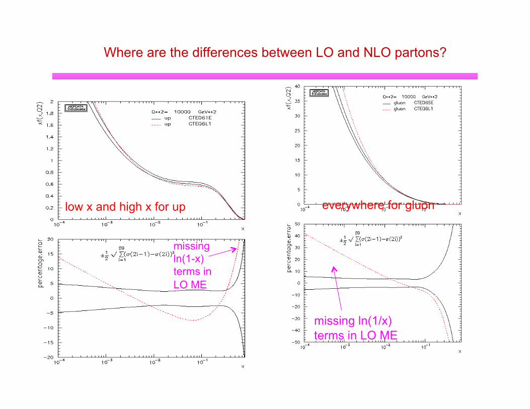
Where are the differences between LO and NLO partons?

low x and high x for up

missing ln(1-x) terms in LO ME

missing ln(1/x) terms in LO ME

everywhere for gluon

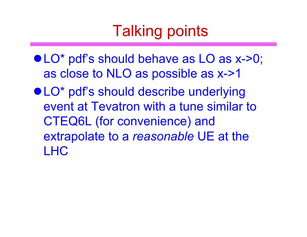
Talking points

 LO* pdf’s should behave as LO as x->0; as close to NLO as possible as x->1

 LO* pdf’s should describe underlying event at Tevatron with a tune similar to CTEQ6L (for convenience) and extrapolate to a reasonable UE at the LHC

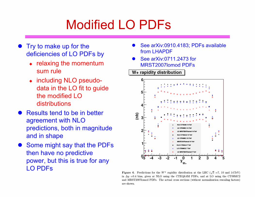
Modified LO PDFs   Try to make up for the

deficiencies of LO PDFs by ◆  relaxing the momentum

sum rule ◆  including NLO pseudo-

data in the LO fit to guide the modified LO distributions

  Results tend to be in better agreement with NLO predictions, both in magnitude and in shape

  Some might say that the PDFs then have no predictive power, but this is true for any LO PDFs

  See arXiv:0910.4183; PDFs available from LHAPDF

  See arXiv:0711.2473 for MRST2007lomod PDFs

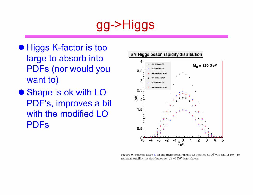
gg->Higgs

 Higgs K-factor is too large to absorb into PDFs (nor would you want to)

 Shape is ok with LO PDF’s, improves a bit with the modified LO PDFs

Tevatron data

  Wealth of data from the Tevatron, both Run 1 and Run 2, that allows us to test/add to our pQCD formalism

  Consider for example W/Z production ◆  cross section increases

with center-of-mass energy as expected

  We’ve already seen that the data is in reasonable agreement with the theoretical predictions

Rapidity distributions  Effect of NNLO is

basically a small normalization shift from NLO

 Data is in good agreement

 Provides some further constraints in pdf fits

Transverse momentum distributions

 Soft (and hard) gluon effects cause W/Z bosons to be produced at non-zero transverse momentum, as we saw last lecture

 Well-described by ResBos and parton shower Monte Carlos ◆  although latter need to

have non-perturbative kT added in by hand

pT distributions   High pT region is due to

hard gluon(s) emission, but is also well-described by predictions such as ResBos

  If we look at average transverse momentum of Drell-Yan pairs as a function of mass, we see that there is an increase that is roughly logarithmic with the mass ◆  as expected from the logs

that we saw accompanying soft gluon emission

Inclusive jet production   This cross section/

measurement spans a very wide kinematical range, including the highest transverse momenta (smallest distance scales) of any process

  Note in the cartoon to the right that in addition to the 2->2 hard scatter that we are interested in, we also have to deal with the collision of the remaining constituents of the proton and anti-proton (the “underlying event”)

  This has to be accounted for/subtracted for any comparisons of data to pQCD predictions

Study of inclusive jet events   Look at the charged particle

transverse momenta in the regions transverse to the dijet direction

  Label the one with the larger amount of transverse momenta the max direction and the one with the smaller amount the min direction

  The momenta in the max direction increases with the pT of the lead jet, while the momenta in the min cone is constant and is approximately equal to that in a minimum bias event

  “Tunes” to the underlying event model in parton shower Monte Carlos can correctly describe both the max and min regions and can be used for the correct subtraction of UE energy in jet measurements

Hadronization   Parton showers in the initial

and final state produce a large multiplicity of gluons

  The parton shower evolution variable t decreases (for the final state) from a scale similar to the scale of the hard scatter to a scale at which pQCD is no longer applicable (near ΛQCD)

  At this point, we must construct models as to how the colored quarks and gluons recombine to form the (colorless) final state hadrons

  The two most popular models are the cluster and string models

• In cluster model, there is a non-perturbative splitting of gluons into q-qbar pairs; color- singlet combinations of q-qbar pairs form clusters which isotropically decay into pairs of hadrons • In string model, relativistic string represents color flux; string breaks up into hadrons via q-qbar production in its intense color field

Herwig Pythia

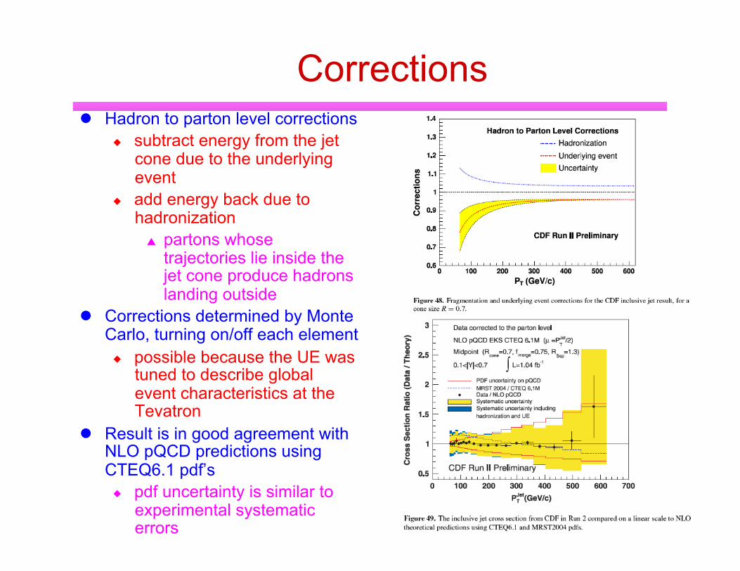
Corrections   Hadron to parton level

corrections ◆  subtract energy from the

jet cone due to the underlying event

◆  add energy back due to hadronization

▲  partons whose trajectories lie inside the jet cone produce hadrons landing outside

…partially cancel, but UE correction is larger for cone of 0.7 hadronization corrections for Pythia and Herwig basically identical

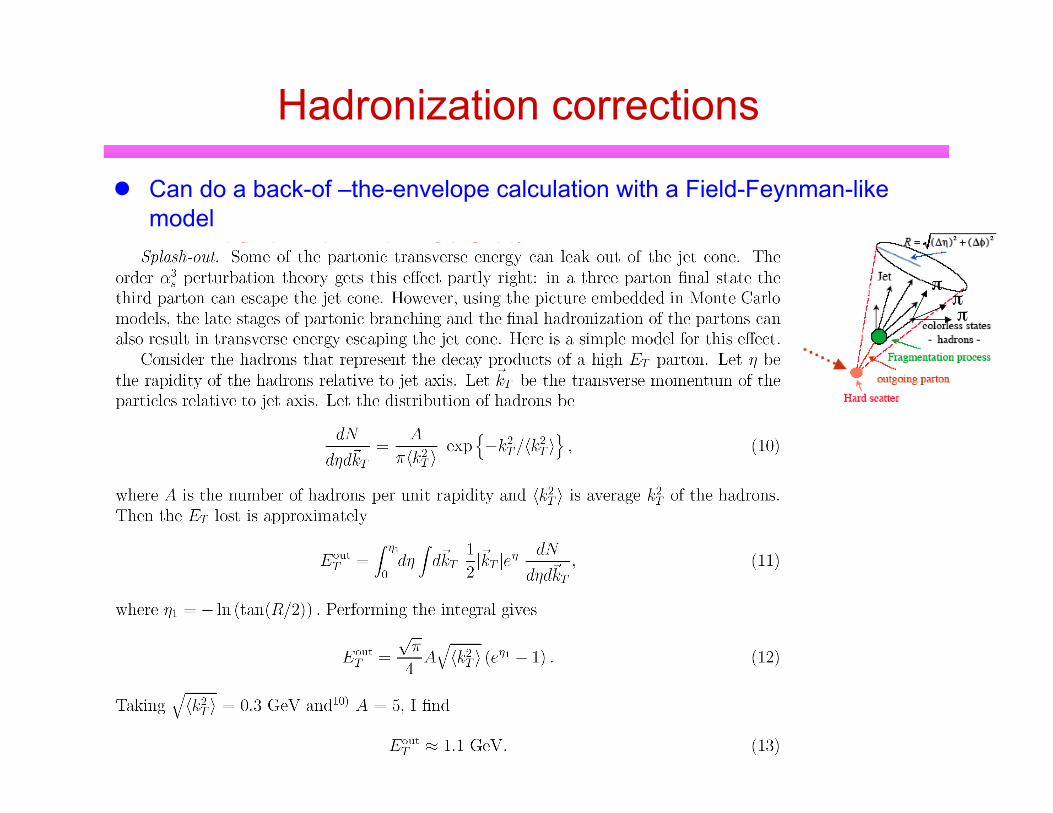
Hadronization corrections

  Can do a back-of –the-envelope calculation with a Field-Feynman-like model ◆  and find on the order of 1 GeV/c

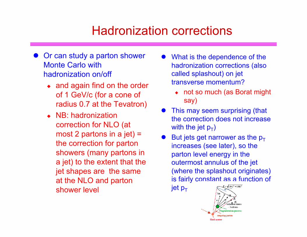
Hadronization corrections

  Or can study a parton shower Monte Carlo with hadronization on/off ◆  and again find on the order

of 1 GeV/c (for a cone of radius 0.7 at the Tevatron)

◆  NB: hadronization correction for NLO (at most 2 partons in a jet) = the correction for parton showers (many partons in a jet) to the extent that the jet shapes are the same at the NLO and parton shower level

  What is the dependence of the hadronization corrections (also called splashout) on jet transverse momentum? ◆  not so much (as Borat might

say)   This may seem surprising (that

the correction does not increase with the jet pT)

  But jets get narrower as the pT increases (see later), so the parton level energy in the outermost annulus of the jet (where the splashout originates) is fairly constant as a function of jet pT

Corrections   Hadron to parton level corrections

◆  subtract energy from the jet cone due to the underlying event

◆  add energy back due to hadronization

▲  partons whose trajectories lie inside the jet cone produce hadrons landing outside

  Corrections determined by Monte Carlo, turning on/off each element ◆  possible because the UE was

tuned to describe global event characteristics at the Tevatron

  Result is in good agreement with NLO pQCD predictions using CTEQ6.1 pdf’s ◆  pdf uncertainty is similar to

experimental systematic errors

Inclusive jet cross section

new physics tends to be central

pdf explanations are universal

crucial to measure over a wide rapidity interval

Full disclosure for experimentalists

  Every cross section should be quoted at the hadron level with an explicit correction given between the hadron and parton levels

note the correction rapidly approaches unity

Jet Shapes   Jets get narrower as the jet pT increases

◆  smaller rate of hard gluon emission as αs decreases (can be used to try to determine αs) ◆  jets switch from being gluon-induced to quark-induced

Jet Shapes: quark and gluon differences

  Pythia does a good job of describing jet shapes ◆  parton showering + hadronization + multiple parton interactions

  If effects of the underlying event are subtracted out, NLO (where a jet is described by at most two partons) also describes the jet shapes well

Quark/gluon jet shape differences

  Quarks and gluons radiate proportional to their color factors

  At leading order

  With higher order corrections, r~1.5

�

r ≡ngnq

≡gluon jet multiplicityquark jet multiplicity

�

r =CA

CF

=94

= 2.25

Jet shapes   Look at the fraction of jet

energy in cone of radius 0.7 that is outside the “core” (0.3)

  Gluon jets are always broader than quark jets, but both get narrower with increasing jet pT

  How to correct for the jet energy outside the prescribed cone? ◆  a NLO calculation “knows”

about the energy outside the cone, so no correction is needed/wanted

◆  for LO comparisons, can correct based on Monte Carlo simulations

at small pT, jet production dominated by gg and gq scattering due to large gluon distribution at low x

Back to jet algorithms   For some events, the jet

structure is very clear and there’s little ambiguity about the assignment of towers to the jet

  But for other events, there is ambiguity and the jet algorithm must make decisions that impact precision measurements

  If comparison is to hadron-level Monte Carlo, then hope is that the Monte Carlo will reproduce all of the physics present in the data and influence of jet algorithms can be understood ◆  more difficulty when

comparing to parton level calculations

CDF Run II events

Jets in real life   Jets don’t consist of 1 fermi

partons but have a spatial distribution

  Can approximate jet shape as a Gaussian smearing of the spatial distribution of the parton energy ◆  the effective sigma ranges

between around 0.1 and 0.3 depending on the parton type (quark or gluon) and on the parton pT

  Note that because of the effects of smearing that ◆  the midpoint solution is

(almost always) lost ▲  thus region II is effectively

truncated to the area shown on the right

◆  the solution corresponding to the lower energy parton can also be lost

▲  resulting in dark towers

remember the Snowmass potentials

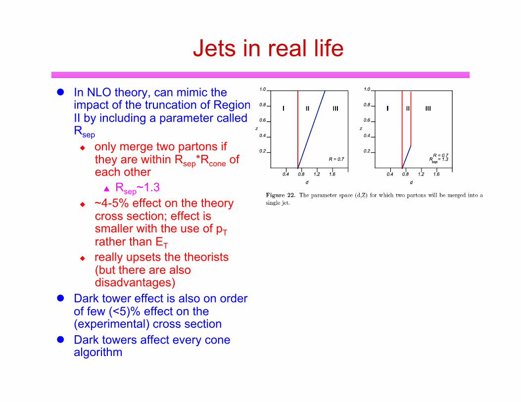
Jets in real life   In NLO theory, can mimic the

impact of the truncation of Region II by including a parameter called Rsep ◆  only merge two partons if

they are within Rsep*Rcone of each other

▲  Rsep~1.3 ◆  ~4-5% effect on the theory

cross section; effect is smaller with the use of pT rather than ET

◆  really upsets the theorists (but there are also disadvantages)

  Dark tower effect is also on order of few (<5)% effect on the (experimental) cross section

  Dark towers affect every cone algorithm

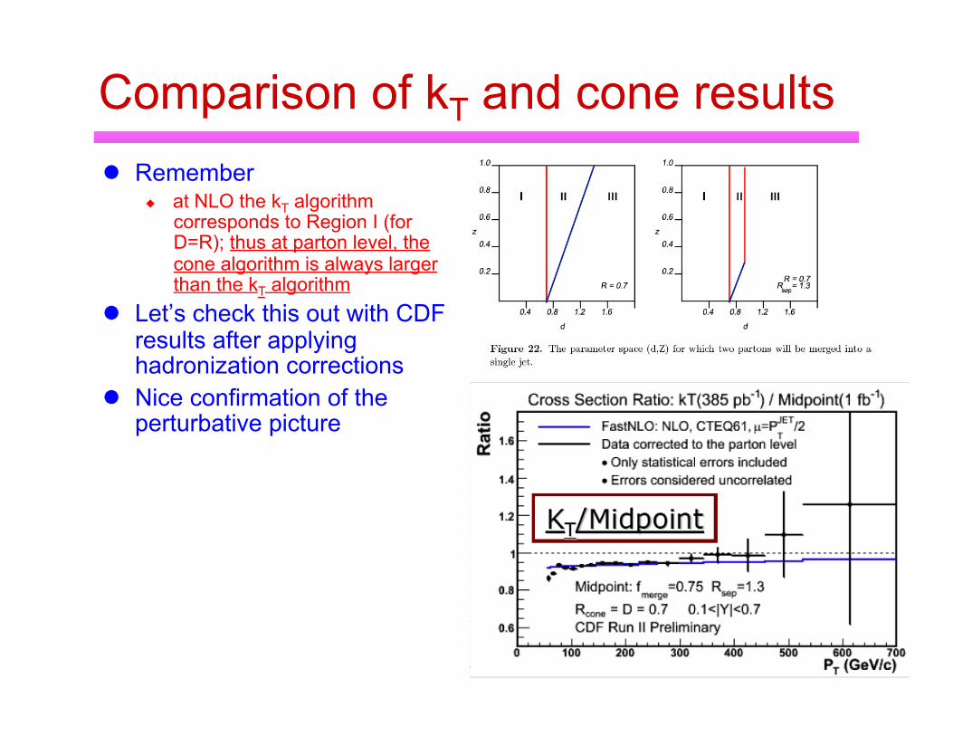
Comparison of kT and cone results   Remember

◆  at NLO the kT algorithm corresponds to Region I (for D=R); thus at parton level, the cone algorithm is always larger than the kT algorithm

  Let’s check this out with CDF results after applying hadronization corrections

  Nice confirmation of the perturbative picture

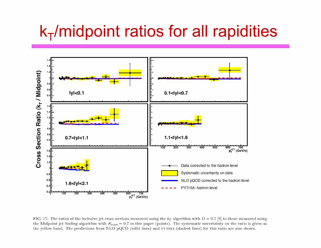
kT/midpoint ratios for all rapidities

SISCone vs Midpoint   The SISCone jet algorithm

developed by Salam et al is preferred from a theoretical basis, as there is less IR sensitivity from not requiring any seeds as the starting point of a jet

  So far, at the Tevatron, we have not explicitly measured a jet cross section using the SISCone algorithm, although studies are underway, but we have done some Monte Carlo comparisons for the inclusive cros sections

  Differences of the order of a few percent at the hadron level reduce to <1% at the parton level

less contribution from UE for SISCone algorithm

SISCone corrections are smaller

New kT family algorithms   kT algorithms are typically slow

because speed goes as O(N3), where N is the number of inputs (towers, particles,…)

  Cacciari and Salam (hep-ph/0512210) have shown that complexity can be reduced and speed increased to O(N) by using information relating to geometric nearest neighbors

  Anti-kT from Cacciari and Salam (reverse kT: Pierre-Antoine Delsart) clusters soft particles with hard particles first

  Now the algorithm of choice for both ATLAS and CMS

�

dij = min pT ,i2p , pT , j

2p( ) ΔRij2

D2

dii = pT ,i2p

p=0; C-A p=1: kT p=-1 anti-kT

Fragmentation functions   On a more inclusive note, can

define a fragmentation function D(z,Q2) that describes the probability to find a hadron of momentum fraction z (of the parent parton) at a scale Q

  The parton shower dynamically generates the fragmentation function, but the evolution of the fragmentation function with Q2 can be calculated in pQCD (just as the evolution of the parton distribution functions can be calculated)

  But, like the PDFs, the value of D(z,Qo) is not known and must be determined by fits to data

  The data from LEP are the most useful for their determination

NB: the gluon fragmentation function is much softer; Herwig does not describe the high z gluon fragmentation function well

Some more details   For outgoing quarks and gluons,

have collinear singularities just as for the parton distribution functions

  Fragmentation functions acquire µ dependence just as PDFs did

  …just like DGLAP

  Lowest order splitting functions are identical to those discussed for PDFs

�

µ 2 ∂∂µ2 Di(x,µ

2) =dzzx

1

∫j∑ αs(µ

2)2π

Djxz,µ 2⎛

⎝ ⎞ ⎠ Pji z,αs µ 2( )( )

Pji z,αs µ 2( )( ) = Pji(0)∫ +

αs µ 2( )2π

Pji(1) z( ) + ...

dσ ppπ

dηdpT2 = fa / p xa,µF( ) ⊗ fb / p∫∫∫ xb,µF( ) ⊗ σ ab→c pT ,

spT2 ,x1,x2,z,

pTµF

, pTµ

⎛ ⎝ ⎜

⎞ ⎠ ⎟ ⊗Dπ / c z,µF( ) × 1+ Ο

m2

pT2

⎛ ⎝ ⎜

⎞ ⎠ ⎟

⎧ ⎨ ⎩

⎫ ⎬ ⎭

�

µ 2 ∂∂µ2 Di(x,µ

2) =dzzx

1

∫j∑ αs(µ

2)2π

Djxz,µ 2⎛

⎝ ⎞ ⎠ Pji z,αs µ 2( )( )

�

Pji z,αs µ 2( )( ) = Pji(0) +

α s µ 2( )2π

Pji(1) z( ) + ...

Calculate single particle cross section by convoluting over fragmentation function

�

dσ ppπ

dηdpT2 = fa / p xa,µF( ) ⊗ fb / p∫∫∫ xb,µF( ) ⊗ σ ab→c pT ,

spT2 ,x1,x2,z,

pTµF

, pTµ

⎛ ⎝ ⎜

⎞ ⎠ ⎟ ⊗Dπ / c z,µF( ) × 1+ Ο

m2

pT2

⎛ ⎝ ⎜

⎞ ⎠ ⎟

⎧ ⎨ ⎩

⎫ ⎬ ⎭

Sum over all fragmentation functions, apply a jet algorithm and voila you have a jet cross section

Photon production   Production doesn’t go out to as high a

transverse momentum as for jets since the cross section is proportional to ααs

  Photons can either be direct or from fragmentation processes ◆  q->qγ

  There are backgrounds from jets which fragment into πo’s which contain most of the momentum (i.e. high z) of the original parton (quarks, not gluons)

  By imposing an isolation cut around the photon direction, the signal fraction can be greatly increased

  The isolation cut can either be a fraction of the photon transverse momentum, or a fixed cut

  To the right, the energy in the isolation cone is required to be less than 2 GeV (corrected for pileup)

◆  this energy is dominated by the UE

Comparison to NLO prediction   Good agreement above 50 GeV/c   Discrepancy below 50 GeV/c   Also seen by D0 and by previous

collider measurements of photon cross sections

  What gives?   Remember the pT of the W; here

we had a two-scale problem (mW and pT

W); near pT~0, the log was large and the effects of soft gluon radiation had to be resummed

kT kick   Here we only have 1 scale (pT

γ) but fixed order pQCD does not seem to be doing well at low pT

  Soft gluons are radiated by the incoming partons as they head towards the hard collision producing the photon ◆  as we saw earlier that the PDF’s

have a Q2 dependence because of this soft radiation

  They reduce the momentum fraction x carried by the parton but also give the parton a transverse momentum

  So that when the two partons collide, they have a relative transverse momentum

  This gives the photon a kT kick, in a manner not described by fixed order pQCD

this kick gets larger as the center of mass increases (and as the mass of the final state increases)

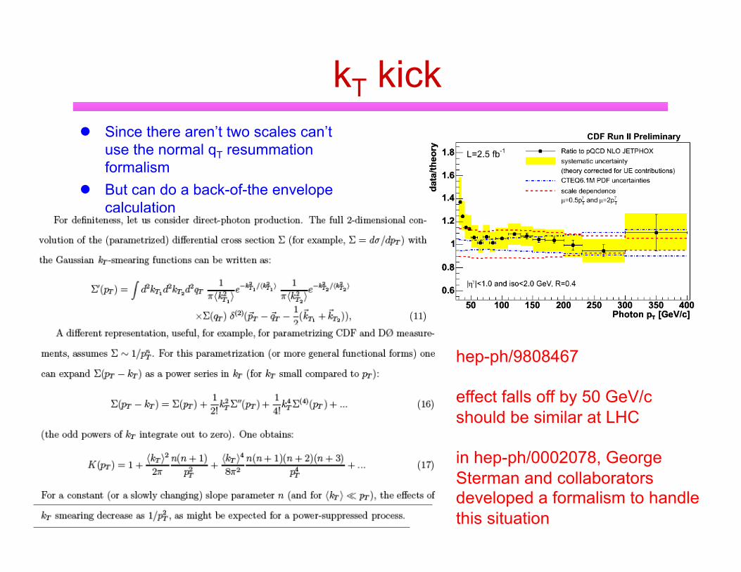
kT kick   Since there aren’t two scales can’t

use the normal qT resummation formalism

  But can do a back-of-the envelope calculation

hep-ph/9808467

effect falls off by 50 GeV/c should be similar at LHC

in hep-ph/0002078, George Sterman and collaborators developed a formalism to handle this situation