LLLeeeccctttuuurrreee 444

INTERUNIVERSITY CENTER FOR SOCIAL SCIENCE THEORY AND METHODOLOGY

Dynamic Networks and Behavior:

Separating Selection from Influence

Christian Steglich

Tom A.B. Snijders

ICS / Department of Sociology,

University of Groningen, The Netherlands

Michael Pearson

Centre for Mathematics and Statistics,

Napier University, Edinburgh

revised version

Groningen, July 18, 2007

[word count: 15434]

ABSTRACT

A recurrent problem in the analysis of behavioral dynamics, given a simultaneously evolving

social network, is the difficulty of separating effects of partner selection from effects of social

influence. Because misattribution of selection effects to social influence, or vice versa, suggests

wrong conclusions about the social mechanisms underlying the observed dynamics, special

diligence in data analysis is advisable. While a dependable and valid method would benefit

several research areas, according to the best of our knowledge, it has been lacking in the extant

literature. In this paper, we present a recently developed family of statistical models that enables

researchers to separate the two effects in a statistically adequate manner. To illustrate our

method, we investigate the roles of homophile selection and peer influence mechanisms in the

joint dynamics of friendship formation and substance use among adolescents. Making use of a

three-wave panel measured in the years 1995-97 at a school in Scotland, we are able to assess the

strength of selection and influence mechanisms and quantify the relative contributions of

homophile selection, assimilation to peers, and control mechanisms to observed similarity of

substance use among friends.

1

INTRODUCTION

In social groups, there generally is interdependence between the group members’ individual behavior

and attitudes, and the network structure of social ties between them. The study of such

interdependence is a recurring theme in theory formation as well as empirical research in the social

sciences. Sociologists have long known that structural cohesion among group members is a good

indicator for compliance with group norms (DURKHEIM 1893, HOMANS 1974). Research on social

identity theory identified within-group similarity and between-group dissimilarity as principles by

which populations are subdivided into cohesive smaller social units (TAYLOR & CROCKER 1981,

ABRAMS & HOGG 1990). Detailed network studies (e.g., PADGETT & ANSELL 1993) as well as

discussion essays (EMIRBAYER & GOODWIN 1994, STOKMAN AND DOREIAN 1997) made clear that

to obtain a deeper understanding of social action and social structure, it is necessary to study the

dynamics of individual outcomes and network structure, and how these mutually impinge upon one

another. In methodological terms, this means that network structure as well as relevant actor

attributes – indicators of performance and success, attitudes and cognitions, behavioral tendencies

– must be studied as joint dependent variables in a longitudinal framework where the network

structure and the individual attributes mutually influence one another. We argue that previous

empirical studies of such joint dynamics have failed to address fundamental statistical and

methodological issues, which may have had undue influence on reported results. As an alternative,

we present a new, statistically sound method for this type of investigation, which we illustrate in an

elaborate empirical application.

The example concerns the joint dynamics of friendship and substance use in adolescent peer

networks (HOLLINGSHEAD 1949, NEWCOMB 1962). It is by now well-established that smoking,

alcohol and drug use patterns of two adolescents tend to be more similar when these adolescents are

friends than when they are not (COHEN 1977, KANDEL 1978, BROOK, WHITEMAN & GORDON

1983). Formulated more generally, people who are closely related to each other tend to be at the

2

same time similar on salient individual behavior and attitude dimensions – a phenomenon for which

FARARO & SUNSHINE (1964) coined the term homogeneity bias. In statistical terminology, this kind of

association is known by the name of network autocorrelation, a notion originating from the spatial

statistics literature (DOREIAN 1989). Up till now, however, the dynamic processes that give rise to

network autocorrelation are not sufficiently understood. Some theorists evoke influence mechanisms and

contagion as possible explanations (FRIEDKIN 1998, 2001; OETTING & DONNERMEYER 1998) – a

perspective largely in line with classical sociological theory on socialization and coercion. Others

invoke selection mechanisms, more specifically homophily (LAZARSFELD & MERTON 1954, BYRNE 1971,

MCPHERSON & SMITH-LOVIN 1987, MCPHERSON, SMITH-LOVIN & COOK 2001) – while still others

emphasize the unresolved tension between these alternative perspectives (ENNETT & BAUMAN 1994,

LEENDERS 1995, PEARSON & MICHELL 2000, HAYNIE 2001, PEARSON & WEST 2003, KIRKE 2004).

Attempts to overcome this tension on the theoretical level are rare and in general not geared to

statistical analysis, but employ simulation (e.g., CARLEY 1991) or analytical techniques (FRIEDKIN &

JOHNSEN 2002). For the empirical researcher, these attempts therefore may not be very helpful.

In order to explain network autocorrelation phenomena, one must take a dynamic

perspective. Considering the case of network-autocorrelated tobacco use, a smoker may tend to have

smoking friends because, once somebody is a smoker, he or she is likely to meet other smokers in

smoking areas and thus has more opportunities to form friendship ties with them (selection). At the

same time, it may have been the friendship with a smoker that made him or her start smoking in the

first place (influence). Which of the two patterns plays the stronger role can be decisive for success or

failure of possible intervention programs – moreover, a policy that is successful for one type of

substance use (say, smoking) may fail for another (say, drinking) if the generating processes are

different in nature. Modeling this as a dynamic process using longitudinal network data is necessary

to address the problem adequately (VALENTE 2003).

3

The most common format of such data in sociological studies is the panel design – which

introduces some analytical complications, because the processes of influence and selection must

reasonably be assumed to operate unobservedly in continuous time between the panel waves. Finally,

complete network studies (i.e., measurements of the whole network structure in a given group) are

clearly preferable to personal (ego-centered) network studies, because selection patterns can best be

studied when also the properties of non-chosen potential partners are known, and because of the

possible importance of indirect ties (two persons having common friends, etc.) that are difficult to

assess in personal network studies. Complete network data have the downside, though, that

individual observations are highly interdependent, which rules out the application of statistical

methods that rely on independent observations – i.e., most standard techniques. To our knowledge,

no previous study succeeded in a statistically and methodologically credible assessment and

separation of selection and influence mechanisms.

In this paper, we show how previous approaches failed to adequately respond to these

statistical-methodological challenges, and we present a new, flexible method that enables researchers

to statistically separate the effects of selection from those of influence. The method, introduced by

SNIJDERS, STEGLICH & SCHWEINBERGER (2007), is based on a stochastic model that formalizes the

simultaneous, joint evolution of social networks and behavioral characteristics of the network actors.

These models can be fitted to data collected in a panel design, where complete networks as well as

changeable attributes are measured. We will call this data type network-behavior panel data,

understanding that ‘behavior’ here stands for changeable attributes in a wide sense, including

attitudes, performance, etc. Model fitting yields parameter estimates that can be used for making

inferences about the mechanisms driving the evolution process. The new method extends earlier

methodology for the analysis of ‘pure’ network dynamics (SNIJDERS 2001, 2005) by adding

components that allow for the inclusion of co-evolving behavioral variables.

4

In addition to the already mentioned network autocorrelation phenomena, other aspects of

dynamic network-behavior interdependence can in principle be investigated with our models. For

instance, GRANOVETTER’s (1982, 1983) theory about weak ties as providers of opportunities for

changing individual properties, or BURT’s (1987, 1992) theory about brokerage and structural

competition, can be tested for their validity on the actor level in a dynamic context where the

network is subject to endogenous change. We hope that the modeling presented here will open new

paths for testing and elaborating such theories. In the present paper, however, we restrict attention

to a general sketch of the modeling framework and one illustrative application, the analysis of

selection and influence mechanisms with respect to substance use behavior (tobacco and alcohol

consumption), based on network-behavior panel data measured in 1995-97 at a secondary school in

Scotland.

Overview

The paper is structured as follows. First, the problem of assessing simultaneously operating selection

and influence processes is illustrated by identifying three major methodological obstacles that need

to be addressed, and giving a summary review and critique of prior research methods. The example

of friendship and substance use in adolescent peer groups will only play a tangential role at this stage.

Then, the actor-driven model family for network and behavior co-evolution is presented on a

conceptual level. For a detailed treatment of the stochastic formalization, we refer to SNIJDERS ET

AL. (2007). We illustrate the new method by applying it to a three-wave data set about the co-

evolution of smoking and drinking behavior with friendship networks (PEARSON & WEST 2003). In

these analyses, selection and influence effects are assessed simultaneously, hence controlling one

effect for the other. A simulation study based on the obtained parameter estimates allows us to draw

quantitative conclusions about the sources of observed network autocorrelation. In addition to

selection and influence on the two substance use dimensions, other possible sources are

5

distinguished: the carryover of network autocorrelation that already existed at the beginning of the

investigated period, selection based on other individual variables (gender, age, money, dating), and

effects of endogenous network formation (reciprocity, balance, and network closure). In the

concluding section, the main results of the article are summarized, and the new method is put into

perspective by hinting at further research areas in which we think the method can be fruitfully

applied.

NETWORK AUTOCORRELATION AS AN EMPIRICAL PUZZLE

The genesis of network autocorrelation is not yet sufficiently understood in many research areas

(MANSKI 1993), and multiple explanatory propositions and theories co-exist. This also holds for the

literature on the effects of peer groups in adolescence, on which we focus here. One can find several

quite specific hypotheses about how friendship networks co-evolve with behavioral dimensions in

general, and with tobacco use and alcohol consumption in particular. The underlying theories posit

conceptually distinct mechanisms which, nonetheless, lead to similar cross-sectional patterns of

network autocorrelation. We confine our review to a short sketch of the three most prominent

mechanisms covered in extant literature – assimilation, homophily, and social context – and the

theoretical background they are typically associated with.

According to socialization theory, peer groups are responsible for creating behavioral

homogeneity in a group (OLSON 1971, HOMANS 1974). The claim is that adolescents, being

influenced by their peers, will assimilate to the peers’ behavior, hence the finding of similarity among

friends. Applications of this strand of theory can be found, e.g., in a series of papers on substance

use by OETTING and co-workers (OETTING & BEAUVAIS 1987, OETTING & DONNERMEYER 1998),

or in HAYNIE’s (2001) analysis of adolescents’ delinquency. In this perspective, change happens

primarily on the individual’s behavior, while the friendship network is treated as rather static

(FRIEDKIN 1998, 2001).

6

A diametrically opposite approach, in which the network is treated as dynamic, but its

determinants as rather static, is taken by research on friendship formation (BYRNE 1971,

LAZARSFELD & MERTON 1954, MOODY 2002). Here, similarity among friends is explained by

selection, i.e., by similar adolescents seeking out each other as friends. There can be different reasons

why this happens. The most widely known is homophily, the principle by which similarity in behaviour

acts as a direct cause of interpersonal attraction (MCPHERSON & SMITH-LOVIN 1987, MCPHERSON

ET AL. 2001). Applications of theories on homophily to adolescents’ substance use can be found, e.g,

in the papers by FISHER & BAUMAN (1988), ENNETT & BAUMAN (1994), ELLIOTT, HUIZINGA &

AGETON (1985), or THORNBERRY & KROHN (1997).

As stressed by FELD (1981, 1982; KALMIJN & FLAP 2001), however, selection patterns that

on the surface look like homophily may in reality result from other selection processes. Different

social contexts (settings, foci) can be responsible for the observed similarity of friends, because when

people select themselves to the same social setting, this usually will indicate prior similarity on a host

of individual properties – while actual friendship formation just reflects the opportunity of meeting

in this social setting, and does not allow us to infer a causal role of the prior similarity in friendship

creation. The argument can be extended to also cover informal forms of social settings, such as the

opportunity structure of meeting others that is implied by the social network itself (PATTISON &

ROBINS 2002). Endogenous mechanisms of friendship dynamics, such as network closure or social

balance (FELD & ELMORE 1982, VAN DE BUNT, VAN DUIJN & SNIJDERS 1999), may this way also

lead to similarity of friends and must not be misdiagnosed as homophile selection patterns (BERNDT

& KEEFE 1995).

In the terminology of BORGATTI & FOSTER (2003), the main dimensions on which these

three accounts of network autocorrelation differ are whether behavior is treated as a consequence

of the network (assimilation) or as its antecedent (homophily, context), and whether temporal

antecedence is also causal (homophily) or only correlational (context). In the case of adolescents’

7

substance use in friendship networks, it is obvious that all three accounts potentially play a role, as

networks typically change a lot during adolescence (DEGIRMENCIOGLU, URBERG, TOLSON &

RICHARD 1998) and the same holds for substance use. As can already be seen from the brief

discussion above, multiple theoretical accounts have been advanced for explaining network

autocorrelation, and a test of these theories against each other is expedient. Considering that previous

research on substance use found evidence for both selection and influence processes, this holds all

the more in the case of our empirical application. In our analyses, we will achieve a separation of

assimilation, homophily and other effects (some related to social context, but also others), on two

substance use dimensions. This separation consists of hypothesis tests of the different

autocorrelation-generating mechanisms in one model, and calculation of model-based effect sizes

for these mechanisms.

Our analysis is certainly not the first attempt to simultaneously assess selection and influence,

and determine the relative strength of each process. However, it differs from previous approaches

by its statistical rigor, and the aim to achieve a methodologically sound separation of selection and

influence effects by employing a model that explicitly represents change in continuous time and the

mutual dependence between network and behavior. Restrictions inherent to our method will be

addressed in the discussion. In the following sections, we will provide reasons why previous, similar

attempts cannot be considered trustworthy. For this aim, a set of criteria (‘key issues’) is derived

which an explanatory model for network autocorrelation should fulfill. The section ends with an

evaluation of previous attempts at disentangling selection and influence, making use of these criteria.

Key issues and a typology of previous approaches

Only a couple of earlier studies tested the competing theories against each other. The earliest

publications on this topic seem to be the articles by COHEN (1977) and KANDEL (1978), which

represent two of the three major previous approaches to the study of network autocorrelation that

8

we propose to distinguish here. These are the contingency table approach (KANDEL 1978, BILLY &

UDRY 1985, FISHER & BAUMAN 1988), ad-hoc social network analysis (COHEN 1977, ENNETT &

BAUMAN 1994, PEARSON & WEST 2003, KIRKE 2004) and structural equation modeling (KROHN,

LIZOTTE, THORNBERRY & MCDOWALL 1996, IANNOTTI, BUSH & WEINFURT 1996, SIMONS-

MORTON & CHEN 2005, DE VRIES, CANDEL, ENGELS & MERCKEN 2006). In the following, these

approaches will be shortly characterized and evaluated against three key issues that are fundamental

for the separation of selection and influence effects. These are incomplete observations implied by the

use of panel data while the underlying evolution processes operate in continuous time, the control

for alternative mechanisms of network evolution and behavioral change in order to avoid

misinterpretation in terms of homophily and assimilation, and network dependence of the actors, which

precludes the application of statistical techniques that rely on independent observations.

To motivate why these are key issues, a consideration of data format requirements for the

task at hand is opportune. It is obvious that longitudinal data are necessary. But how does the choice

for a specific type of data relate to the objective of separating selection from influence? If the whole

process of network evolution and adjustment of behavior were traced in continuous time, little

ambiguity would be left about whether selection or influence occurs at any given moment: network

changes give evidence of selection processes, behavior changes indicate influence processes.

Unfortunately, panel data, measured at only a few discrete time points, are the most common

longitudinal format in sociological studies, and social network research is no exception to this rule.

The temporal incompleteness of panel data makes it impossible to unequivocally identify which

process is responsible for an observed change, even if only the network or only the behavior changes

from one observation to the next – simply because a change on the respectively other dimension may

also have happened, but there has been a change back to the original value afterwards during the

same period. The two columns on the left in Figure 1 illustrate such situations. Suppose that the pair

of pupils in the middle column is observed at moments t0 and t1. At both moments, they are non-

9

drinkers, but while they are unconnected at t0, there is a unilateral friendship tie between them at t1.

At first sight, one might diagnose a pattern of homophile selection. However, the unobserved

process that generated these data may have looked fundamentally different, as illustrated in the

brackets. A while after the observation at t0, the actor on the right may have started drinking, say,

because he didn’t have any friends. The actor on the left may have noticed that and started a

therapeutic friendship with the new drinker. Under these circumstances, the drinker quit drinking

again. Only now, the network is observed again at t1. In this scenario, the processes actually

happening have nothing to do with homophile selection, and to diagnose the observations as

unequivocal evidence for selection is plainly wrong. Nonetheless, literally all quantitative studies on

the topic that we are aware of commit this error. As the example illustrates, alternative mechanisms

of network formation as well as behavior change need to be controlled for in order to preclude such

misinterpretation. A similar scenario, sketched in the left of Figure 1, illustrates how homophile

selection (taking place shortly before observation moment t1) can be misdiagnosed as the occurrence

of social influence (the default interpretation of the observed data when the happenings in the

brackets are neglected). The longer the time intervals are between observations, the higher the

chances that such alternative trajectories happen. In the studies on adolescent behavior mentioned,

time intervals of one year are the rule – while scenarios as sketched in Figure 1 can reasonably be

assumed to take place within a few months. The use of retrospective questions for assessing the

particular relationship’s history (KIRKE 2004) in principle could remedy this predicament. However,

retrospective social network information is rare and prone to unreliability (BERNARD, KILLWORTH,

KRONENFELD & SAILER 1985), so this remedy leads to other problems.

> Insert Figure 1 about here. <

It should be noted that the problem of alternative generating mechanisms is not limited to

situations where the data are incompletely observed. In the column on the right of Figure 1, the

newly created tie could result from homophile selection (and indeed would be unequivocally

10

diagnosed as such by previous approaches in the literature). However, it also could result from a

purely structural mechanism known to play a strong role in friendship formation, namely triadic

closure. Having a common friend at t0 may be the reason why at t1, a tie is established between the

two previously unrelated actors. The message is that even if we can assume that no unobserved

changes have taken place, there still is interpretative leeway concerning the mechanisms responsible

for a given observed change. Controlling for such mechanisms as far as possible is a criterion that

previous research largely has failed to address.

Next to the temporal aspect of data collection, also the cross-sectional design is of

importance for the prospect of distinguishing selection from influence effects. There are two major

types of social network studies, one being the ego-centered network studies, in which for a random

sample of individuals, the network neighbors and their properties are assessed. The other type are

the complete network studies, in which for a given set of actors (the egos), all relational links in this

set are assessed. For the present purpose, the collection of ego-centered network data is inadequate

because even in a panel study, such data do not provide information about other, potential relational

partners that were not selected. This precludes a meaningful assessment of selection processes. For

adequately measuring selection effects, a meaningful approximation of the set of potential relational

partners must be made, whose individual properties must be known irrespective of whether they

actually become partners or not. In studies of complete networks, these data are available for all

actors in the network. Following from the above consideration, a necessary condition for conducting

a complete network study is that the delineation of the network gives a reasonable approximation

to the set of the actual and potential relational partners. However, this information comes at the

price of dependence of observations, which rules out the application of the common statistical

procedures, as these rely on randomly sampled data. Depending on the exact nature of the data, such

procedures can be biased towards conservative as well as liberal testing (KENNY & JUDD 1986,

BLIESE & HANGES 2004), and therefore lack reliability.

11

An assessment of previously used analytical methods

There are earlier attempts to separate selection effects from influence effects, which above we

categorized in three main groups: modeling frequencies in a contingency table, ad-hoc applications

of social network analysis, and structural equation modeling. Here, we will shortly characterize these

methods, in this order, and highlight the degree to which they meet the requirements on the three

key issues introduced.

In the contingency table approach, typically dyads of mutually-chosen best friends are cross-

tabulated according to whether or not the two pupils’ friendship remains stable between first and

second measurement, and whether or not their behavior falls in the same, binary category. Influence

is typically assessed by studying the subsample of respondents who named the same best friend in

both waves, while selection is assessed on the subsample of changing friendship ties. For both

mechanisms, probabilities of change towards a behaviorally homogeneous friendship are calculated,

and based on these probabilities, predictions are generated for the whole sample of dyads.

Significance tests for the two mechanisms then are derived by comparing these predictions to the

observed data, under the assumption of dyad independence. Prominent studies that employ variants

of this approach are KANDEL’s (1978) seminal study of marijuana use, educational aspirations,

political orientation, and delinquency at New York State high schools, BILLY & UDRY’s (1985) study

of adolescents’ sexual behavior, and FISHER & BAUMAN’s (1988) investigation of adolescents’

smoking and alcohol consumption. Our key issue of network dependence, here in the shape of

inadequately assuming dyad independence, usually is acknowledged as an acceptable weakness in this

research. The two other key issues, though, remain fully unaddressed. Especially the use of

incompletely observed data puts a question mark over the results. Because the categorization of

dyads in the contingency table is based only on the observed states at the beginning and at the end

of the observation period, the possibility of multiple explanatory trajectories linking these

observations (as shown in Figure 1) is ruled out, unduly so. Alternative generating mechanisms,

12

finally, can to some degree be controlled for in this approach (see FISHER & BAUMAN 1988 for an

example). However, triadic effects such as network closure or balance cannot, because of the

restriction to dyads.

The studies we summarize as taking an ad-hoc social network analysis approach follow an explicit

two-stage strategy. First, the network data are collapsed into summary statistics on the actor level,

indicating the actors’ network position and properties of his network neighborhood. Second, these

reduced data are analyzed. Implicit in this approach are (usually inappropriate) assumptions that all

change is observed and sufficiently reflected in the chosen statistics. The secondary analyses are

typically based on independence assumptions which clearly are erroneous, so that the studies cannot

establish a firm statistical conclusion concerning processes of influence and selection. Next to leaving

all our key issues unresolved, however, there are additional problems with this approach. One is

related to the arbitrariness in the choice of the particular pre-processing algorithm. While ENNETT

& BAUMAN (1994), PEARSON & MICHELL (2000) and PEARSON & WEST (2003) make use of the

NEGOPY software (RICHARDS 1995), which categorizes respondents into the four sociometric

positions ‘group member’, ‘peripheral’, ‘liaison’ and ‘isolate’, COHEN (1977) relies on a definition of

sociometric groups proposed by COLEMAN (1961), while KIRKE (2004) relies on the identification

of weak components provided by the GRADAP software (SPRENGER & STOKMAN 1989). The

different options available at this pre-processing stage are manifold, and their consequences are not

well-understood. More importantly, though, the reliance on the output of such algorithms implies

that network positions and neighborhood properties are used as if they were exogenously determined

actor attributes. Further mutual interdependencies in the network structure, or the specific identity

of the peers, are not taken into account. A ‘group member’ at one observation may still be identified

as a ‘group member’ at the subsequent observation, yet the groups referred to may consist of

completely different peers. In such a situation, even the assumption that ‘the group’ exerted social

influence in the period in-between seems dubious. Also, the selection of specific peers cannot be

13

modeled in an actor-based analysis, and accordingly, the study of influence processes is not

controlled for selection. As partial solution to the problem of peer identity, the actor-level statistics

obtained in the first stage can be combined with an analysis on the dyad level under a contingency

table approach (see ENNETT & BAUMAN 1994 for an example).

The third type of studies that we distinguish here employ structural equation models to assess

selection and influence (KROHN ET AL. 1996, IANNOTTI ET AL. 1996, SIMONS-MORTON & CHEN

2005, DE VRIES ET AL. 2006). An advantage of this approach over the other two is the relative ease

to simultaneously assess selection and influence effects in the same analysis, controlling one for the

occurrence of the other. Typically, ‘cross-lagged’ model specifications are used to estimate effects

of previous-wave respondent behavior on current-wave peer behavior, and previous-wave peer

behavior on current-wave respondent behavior. In this setup, the estimated path coefficient from

lagged peer behavior to current respondent behavior is taken as a measure of peer influence, while

the coefficient for the path from lagged respondent behavior to current peer behavior is taken as an

indicator for selection effects. By estimating separate effects for old friends and new friends, the

interpretation of path coefficients in terms of selection and influence is possible, at least

conceptually. However, the method still neglects the three key issues of incomplete observations

(estimated path coefficients directly link the observed variables to each other), alternative generating

mechanisms (triad effects not possible to include), and – here especially important – the

interdependence of observations. When analyzing complete network data, the individual respondent,

whose behavior figures central in one observation, will appear again among the peers for other

observations. This clearly violates independence of observations, which is one of the crucial

assumptions of structural equation modeling. While the use of ego-centered data would solve this

problem, it is not an option because it effectively precludes the study of selection processes, as

outlined earlier.

14

To summarize: the three analytical strategies covered here all follow a two-stage procedure.

In the first stage, the network data are collapsed into individual-level variables (e.g., local density,

centrality, indicators of group position, peer behavior) or dyad-level variables (behavioral

homogeneity), which in the second stage figure as variables in more conventional analyses – as

dependent variables for assessing selection effects, and as independent variables for assessing effects

of social influence. The shortcomings of such approaches are related to the key issues introduced

earlier. The stage of collapsing networks into individual- or dyad-level data remains arbitrary does

not do full justice to structural aspect of evolving networks. In particular, the use of such collapsed

variables artificially freezes their values at the last preceding observation, which negates their

endogenous nature and inhibits the study of potentially important feedback mechanisms between

network and behavior that are unobserved. Alternative mechanisms that may be responsible for

observed changes are generally difficult to include in the models, especially when they express triadic

or higher-order network effects such as closure or structural balance. Finally due to the problem of

non-independence of actors and dyads, the first step of data reduction does not deliver data that

meets the requirements of the statistical procedures applied in the second-stage analyses.

A NEW APPROACH:

MODELING THE CO-EVOLUTION OF NETWORKS AND BEHAVIOR

The following requirements are desirable for a more suitable model for analyzing network-behavior

co-evolution. First, the model must allow for unobserved changes to occur in-between the

observation moments. Second, the model must be able to express the feedback processes consisting

of the simultaneously operating effects of the network on the behavior of the actors, and of the

behavior on the network. Third, the interdependence of actors in the network needs to be taken into

account. Basic types of such interdependence are the dependence of all ties involving one given

actor, and network closure. In order to keep track of these interdependencies, collapsing the network

15

into a vector of summary characteristics per actor or per dyad is inadequate, but rather the evolution

of the complete network-behavior data structure should be modeled as a complex whole. A

computational model, which can be analyzed by means of computer simulations, is likely the only

satisfactory way to proceed.

This is achieved by the method proposed by SNIJDERS ET AL. (2007), which is an extension

of earlier modeling work by SNIJDERS (2001, 2005) for networks without co-evolving behavioral

dimensions. The process of network-behavioral co-evolution is modeled here as an emergent group

level result of interdependent behavioral changes occurring for single actors, and network changes

occurring for pairs of actors. The model assumes that changes may occur continuously between the

observation moments. Handling the dynamic mutual dependence of the network ties and the

individual behavior requires a process model that specifies these dependencies in a plausible way.

Specifying this as an actor-based model makes sense in a lot of applications, as it is in line with extant

theories of individuals who act in the context of a social network. E.g., for the study of friendship

networks, taking the network actors as the foci of modeling seems natural, as commonly invoked

mechanisms of friendship formation (like homophily, reciprocity or transitive closure) are

traditionally formulated and understood as forces operating at the actor level, within the context of

the network; the same holds for mechanisms of behavioral change (like social influence). Modeling

these changes in an actor-based framework implies that actors are assumed to “make” the change,

by altering either their outgoing network ties or their behavior. The central model components will

be the actors’ behavioral rules determining these changes.

Action rules and occasions to act

Some assumptions need to be made in order to retain a tractable model. While we focus on the

analysis of data measured at discrete time points, we assume that in the underlying dynamic process,

changes in network ties and behavior happen in continuous time, at stochastically determined

16

moments. This allows us to tackle the key issue of unobserved changes. Distinguishing between the

network changes of an actor and his behavior changes, we rule out the possibility that changes in

network ties and in actor behavior, or changes by two different actors, occur at the same time point.

An example for such forbidden simultaneous changes would be binding contracts of the type “when

you start smoking, I’ll become your friend.” While such bargaining is not impossible, we will here

model it as two subsequent changes, the connection of which cannot be enforced. Given the present

application of the model to the evolution of substance use and friendship ties, such an assumption

seems reasonable – in other applications, it could be relaxed. The compound change that is observed

between two observations thus is interpreted as resulting from many small, unobserved changes that

occurred between the observation moments. The assumption that at any given moment, not more

than one tie variable or one behavior variable can change, enables us to keep the rules that govern

actors’ behavior relatively simple, relieving us from the burden of explicitly modeling the totality of

changes between two measurements all at once (an advantage of continuous-time modeling put

forward already by COLEMAN, 1964). Here, this assumption provides an elegant and simple way of

expressing the feedback processes inherent in the dynamic process, where the currently reached state

is also the initial state for further developments, and where the probabilities for specific changes can

depend, in perhaps complicated ways, on the entire current network-behavior configuration. There

is a cost to this approach, however. Because we cannot know which precise trajectory of small

changes happened from one observation to the next, we have to rely on data augmentation

procedures and simulation-based inference for estimating our models. Spelling out a probability

model for all possible trajectories between the observed states allows such inference, and it becomes

possible to infer effect sizes of various mechanisms operating in the process, and test hypotheses

about them. So, the key issue of alternative generating mechanisms can be addressed adequately. The

first observation in the panel data set is not modeled but conditioned upon, i.e., the starting values

of the network ties and the initial behavior are taken for granted. This implies that the evolution

17

process is modeled without contamination by the contingencies leading to the initial state, and that

no assumption of a dynamic equilibrium needs to be invoked. For changes of network as well as

behavior, we now proceed to modeling the temporal occurrence of opportunities for the different types

of changes, and the rules of change followed by the actors, once they face such an opportunity.

> Insert Table 1 about here. <

These model components, summarized in Table 1, will be sketched below in a formal probabilistic

operationalization, using the application to substance use in high school as an illustration. Formally,

the model is a continuous time MARKOV process, where the totality of possible combinations of

network ties and actor behavior figures as the state space. While the model in principle is equipped

for analyzing the co-evolution of multiple dimensions of networks and behavior, we consider – for

ease of presentation – the case of one network variable X and one dependent actor variable Z only

(in the empirical section, we will give an example with two behavioral dimensions). In the following,

first some notational conventions are introduced, and then the formal model is sketched. A detailed

mathematical account of our model is given in SNIJDERS ET AL. (2007).

Notation and data requirements

The outcome variables for which the model is defined are the changing network and the changing

actor behavior – which may be called endogenous, since they evolve as a function of each other – and

independent variables that can be individual, dyadic, changing or unchanging. We make use of the

following notation. The network is assumed to be based in a group of N actors – e.g., a cohort of

pupils at the same school, or business firms active in the same period in the same industry. The

network is denoted by x, where xij(t) stands for the value of the directed relationship between actors

i and j at time point t. Examples for such relational variables are friendship between the pupils of a year

group, advice among employees in an organization, or share ownership between business firms. We

assume that x is dichotomous, i.e., xij=1 stands for presence of a tie and xij=0 for absence. Next, z

18

denotes the behavioral variable, with zi(t) standing for the score of actor i at time point t. Examples

here are the smoking behavior of pupils, the performance of employees, or the activity in a given market

segment of a business firm. We assume that behavioral dimensions are measured on a discrete, ordinal

scale represented by integer values (including dichotomous scales). Finally, v and w denote actor-level

and dyad-level exogenous covariates, respectively (for ease of presentation here assumed to be

constant over time), with standing for the score of actor i on actor covariate k, and ( )k

iv( )k

ijw

standing for the dyadic covariate k measured for the pair (ij). Typical actor covariates are gender, age

or education of a pupil or an employee, or number of employees of a business firm. Examples for dyadic

covariates could be a classmate relation between pupils in a year group, an organizational hierarchy between

employees, or the geographical distance of business firms.

We consider the case of network-behavior panel data, where the network and behavioral data are

collected for a finite set of time points only (say, t1<t2<...<tM), with at least M=2 waves. In the

following, the data are indicated by lowercase letters (networks x(t1),...,x(tM), behavior z(t1),...,z(tM),

etc.), while the stochastic model components (of which these data are assumed to be realizations) are

indicated by uppercase letters (network model X(t) and behavioral model Z(t)). Note that the formal

model itself will describe network evolution in continuous time, notwithstanding the fact that it is

used for the analysis of observations at discrete time points. The formal model is obtained by spelling

out the submodels indicated in Table 1 and integrating them into the overall model. Although the

objective functions are the most important model component, for ease of presentation we first

explain the model for occurrence of changes.

Modeling opportunities for change

The assumption was already mentioned that at any single moment, only one tie variable or one

behavioral variable may change. More specifically, it is assumed that at stochastically determined

moments, one actor gets the opportunity to change one of his/her outgoing tie variables, or to

19

change his/her behavior. Such opportunities for change are called micro steps. It also is allowed that

the actor does not make a change but leaves things as they are. The frequency by which actors have

the opportunity to make a change is modeled by rate functions, one for each type of change. The

main reason for having separate rate functions for the behavioral and the network changes is that

practically always, one type of decision will indeed be made more frequently than the other. In

information flow networks, for example, one can expect that the actors’ individual properties (here:

knowledge states) change more quickly than their network ties. In group formation processes, where

the behavioral dimensions may represent attitudes, the opposite may be true. In the application to

substance use and friendship at high school, one would expect quicker changes in the network than

in substance use, caused by (a) the addictive nature of substance use and (b) the students’ social

orientation phase in adolescence.

The first observations of network ties x(t1) and behavior z(t1) serve as starting values of the

evolution process – i.e., they are not modeled themselves, but conditioned upon, and only the

subsequent changes of network ties and behavior are modeled. The timing of the micro steps is

modeled by the following stochastic process. For each actor i and for network and behavioral changes

alike, we model the waiting time until actor i takes a micro step by exponentially distributed variables

Tinet and Ti

beh with parameters λλλλinet>0 and λλλλi

beh>0, i.e., the waiting times are distributed such that

for all t>0. The parameters of these distributions indicate the rate (or speed)> = −Pr( ) exp( )T t tλλλλ

at which the respective change is likely to occur; the expected waiting time is 1/λλλλ. Exponential

waiting times are a standard assumption for this type of stochastic processes. Since actual waiting

times between changes are not observed, more complicated modeling is unwarranted. It is further

assumed that all waiting times are independent, given the current state of network and behavior.

Properties of the exponential distribution imply that, starting from any given moment in time (e.g.,

the time when the preceding micro step occurred), the waiting time until occurrence of the next micro

step of either kind by any actor is exponentially distributed with parameter .( )net beh

total= +∑ i ii

λ λ λλ λ λλ λ λλ λ λ

20

The probability that this is a network micro step taken by actor i is , and the probabilitynet

total/

iλ λλ λλ λλ λ

that it is a behavioral micro step taken by actor i is . beh

total/

iλ λλ λλ λλ λ

There may be heterogeneity in the activity of actors – some actors may change their network

ties, or their behavior, more quickly than others. Such activity differences may be caused by individual

properties (e.g., by gender differences) or by existing network structure (e.g., by the number of ties

an actor already has). We can directly incorporate such activity differences between actors by allowing

actor covariates and the current network positions to exert an influence on the rate functions by

letting the parameters λλλλ depend on actor attributes and network positions, see SNIJDERS (2001, 2005).

In this paper, however, we limit the discussion to model specifications where both types of rate

functions are constant across actors and network positions, and depend only on the periods between

panel waves.

Modeling mechanisms of change

What happens in a micro step is modeled as the outcome of changes made by the actors. Micro steps

can be of two kinds, corresponding to network changes or behavioral changes. For network changes,

the micro step consists of the change of one tie variable by a given actor. Say, x is the current network

and actor i has the opportunity to make a network change. The next network state x' then must be

either equal to x (i.e., keep the current situation) or deviate from x in exactly one element in row i

(i.e., change the tie variable linking actor i to one other actor). From these N possible outcomes, it

is assumed that i chooses that value x' for which is maximal. Here z isεεεε′ ′+net net( , , ) ( , , )i if x x z x x z

the current vector of behavior scores, is a deterministic objective function that can benetf

interpreted as a measure of the actor’s satisfaction with the result of the network decision (“what the

actor strives for, behaviorally”), and is a random disturbance term representing unexplainednet

εεεε

change. By making some convenient standard assumptions about the distribution of the random

21

component (MCFADDEN 1974, PUDNEY 1989), the choice probabilities can be expressed in

multinomial logit shape, as proportional to .( )′netexp ( , , )if x x z

In a behavioral micro step, it is assumed that a given actor either increments or decrements his

score on the behavioral variable by one unit, provided that this change does not step outside the

range of this variable; it is also allowed that the score is not changed. The modeling is completely

analogous to that of the network micro steps. If z is the current vector of behavior scores for all

actors, and i is the actor allowed to change his behavior, let z' denote the vector resulting from an

allowed micro step. It is assumed that i chooses that value z' for which εεεε′ ′+beh beh( , , ) ( , , )i if x z z x z z

is maximal, where now is a (different!) deterministic objective function that again can bebehf

interpreted as the actor’s satisfaction with the result of the behavioral decision, and again is aεεεεbeh

random disturbance term representing unexplained change. By making appropriate assumptions about

the distribution of the random component, choice probabilities can also be expressed in multinomial

logit shape. It may be necessary to point out here that the model formulation in terms of choice

models does in no way imply that we assume actors to be strategically rational, let alone that estimated

parameters for the objective functions express respondents’ actual preferences. This and more

cautioning remarks about model interpretation will be addressed in more detail below.

The focus of modeling is on the deterministic parts, defined by the objective functions f. A

high degree of flexibility is achieved by modeling these as linear combinations of effects that express

the dependence of network and behavior on each other as well as on externally given variables. The

term exogenous will be used for effects depending on such external variables, while endogenous effects

depend on the current values of the dependent variables (networks and behavior). For network

changes, the objective function has the general shape , where′ ′=∑net net net( , , ) ( , , , )i h hhf x x z s i x x zββββ

statistics stand for the effects, weighted by parameters whose size is determined by fittingnet

hsnet

hββββ

the model to the data. Analogously, the objective function for behavioral changes has the form

. The statistics, or effects, must be defined on substantive′ ′=∑beh beh beh( , , ) : ( , , , )i h hhf x z z s i x z zββββ

22

grounds, and are arbitrary from the point of view of mathematical modeling, although in practice it

is an advantage that they are not too complicated computationally. The most important network and

behavior effects do not depend on the previous states x' and z' but only on the new states x and z,

and their weights ββββ can be interpreted as the degree to which the actors have a tendency to change

into a direction where the network-behavioral state has high values for these effects. A selection of

possible endogenous network effects is given in Table 2, while a similar selection of effects net

hsbeh

hs

for behavioral changes is given in Table 3. These components are based on indicators of structural

positions in networks that are of fundamental importance in social network analysis (WASSERMAN

& FAUST 1994). The second column of these tables contains the formulae of the statistics that express

the respective effects.

> Insert Tables 2 and 3 about here. <

In these tables, similarity of the behavioral scores of two actors i and j is defined as

, where the range of behavioral scores is defined as the maximum minus: 1sim range= − −ij i j Z

z z

the minimum of observed values. By this definition, similarity is standardized to the unit interval,

sim=0 indicating maximally dissimilar scores and sim=1 indicating identical (i.e., maximally similar)

scores. For the calculations of the statistics in the tables, similarity is further centered around the

empirical average over all measurement points. Such centering reduces estimation difficulties caused

by collinearity. Therefore, also the covariates and behavioral variables are centered (which, in this

case, can be seen back in the formulae). The balance effect for network evolution contains a measure

of structural similarity that is analogous to similarity, where b is( )strsim := − −∑ij h ih jhb x x

a parameter used for standardization (DAVIS 1963, MIZRUCHI 1993). In network terms, this may be

regarded as a measure for structural equivalence as regards outgoing ties (LORRAIN & WHITE 1971).

The tables can naturally only give a glimpse of the complexity and richness of modeling that becomes

possible within the proposed framework. The range of research questions that can be analyzed this

way will give rise to many more effects that cannot be covered here.

23

Integration of model components

The total model specification for network-behavioral co-evolution consists of the first wave

observations x(t1) and z(t1) as initial state of the stochastic process, the rates of occurrence of network

or behavioral micro steps by specific actors as sketched above, and the choice probabilities for each

possible micro step. As a whole, the model belongs to the class of continuous time Markov chains (e.g.,

NORRIS 1997). The description given above allows us to construct a computer simulation of this

process and also to specify the so-called intensity matrix which is the mathematical characterization

of the Markov chain process.

The model is too complicated to allow for closed-form calculations of probabilities,

expectations, etc. Direct ways of parameter estimation such as maximum likelihood are therefore not

easily implemented. However, once tentative parameter values are assumed, the evolution model can

be implemented as a stochastic simulation algorithm which can be used to generate network and

behavioral data according to the postulated dynamic process. Then, parameter estimates can be

determined as those values under which simulated and observed data resemble each other most

closely. In statistical terminology, this is called the method of moments. The resemblance criteria are

crucial for the estimation procedure, which is described in detail in SNIJDERS ET AL. (2006). Parameter

estimation for this type of model has been broadly categorized as “third generation problems” in

applied statistics (GOURIÉROUX & MONFORT 1996) and is computationally intensive. Depending on

the data set, it is possible that for some models, the algorithm does not converge in a satisfactory way.

This happens for models that are complicated in the sense that there are too many parameters relative

to the variation in the data, or when effects are highly correlated in the data. Non-convergence may

also be an indicator of model misspecification. In the large majority of cases, however, with data sets

ranging between 30 and a few hundred actors, our experience is that convergence results are good.

24

Interpretation of model parameters

As a consequence of the actor-driven nature of modeling, special attention needs to be paid to the

interpretation of the estimated model parameters. The parameters of the rate functions can be related

transparently to the speed of the evolution process. The parameters of the objective functions,

however, relate in a more indirect way to the observed global dynamics of network and behavior.

From a perspective of agency, these functions can be regarded as satisfaction measures of the actors

with their local network-behavioral neighborhood. At a less construing level, they can be thought of

descriptively, as those behavioral rules that are likely followed by the actors, given the observed data.

These objective functions, together with the current network-behavior configuration, imply specific

global dynamics as emergent property of the individual changes, in which network actors are mutually

constraining each other and mutually offering opportunities to each other in a complicated feedback

process. In order to understand how the estimated parameters of the objective functions relate to the

global dynamics observed, the Markov property of the process model needs to be invoked. This

property implies that corresponding to the parameters there is a stationary (equilibrium) distribution

of probabilities over the state space of all possible network-behavior configurations. Because often,

the data configuration observed in the first wave of the panel will not be in the center of this

equilibrium distribution, the model defines a non-stationary process of network-behavioral dynamics,

starting at the first observation, and then ‘drifting’ towards those states that have a relatively high

probability under the equilibrium distribution – for the mathematical principles, see e.g. NORRIS

(1997). The dynamics as well as the stationary distribution of all but the simplest cases of these

models are too complex for analytic calculations, but they can be investigated by computer

simulation.

For the ‘immediate interpretation’ of the objective functions’ parameters, it can be useful to

consider the odds of somewhat idealized micro steps (this is similar to the interpretation of

parameters obtained by logistic regression). Suppose an actor i is in a situation to make a network

25

micro step, and suppose two alternative courses of action result in networks and . From theAx Bx

linear shape of the objective function and the multinomial logit probabilities for micro steps, the odds

for these outcomes can be derived as , in( )net net netPr( ) Pr( ) exp ( ) ( ) = − ∑A B h h A h Bhx x s x s xββββ

simplified notation. As can be seen from this formula, the odds depend on the degree to which the

two networks differ on the actor-specific statistics (see Table 2), these differences being weightednet

hs

by the model parameters. Likewise, if the actor is in a situation to make a behavioral micro step, and

considering two alternative courses of action resulting in behavioral vectors and , the oddsAz Bz

are given by . ( )beh beh behPr( ) Pr( ) exp ( ) ( ) = − ∑A B h h A h Bhz z s z s zββββ

By way of example, let us assume that in a simple model specification, the function

was estimated as typical network′ ′ ′ ′= − + +∑ ∑ ∑net ( , , ) 2.0 2.5 1.0 simi ij ij ji ij ijj j jf x x z x x x x

objective function, while the behavioral objective function was estimated as

, also quite typical. The( ) ( )beh 2( , , ) 1.0( ) 0.5( ) 2.5 sim′ ′ ′ ′= − − − − + ∑ ∑i i i ij ij ijj jf x z z z z z z x x

primes indicate those elements in the formulae the values of which are under the control of actor i

and may be changed in a micro step that is governed by the objective function in which they occur.

The network objective function contains three effects: the outdegree effect (with parameter estimate

), the reciprocity effect (with parameter estimate ), and the similarity effect= −net

out 2.0ββββ =net

rec 2.5ββββ

(with parameter estimate ). In the behavioral objective function, the model contains three=net

sim 1.0ββββ

more effects: two parameters determining the basic shape of the distribution of the variable, one

linear (with estimate ) and one quadratic (with estimate ) , and an effect ofbeh

lin 1.0= −ββββ beh

quad 0.5= −ββββ

average similarity to neighbors (with parameter estimate ). We now address the questionbeh

av.sim 2.5=ββββ

of how these parameter values can be interpreted, starting with the network objective function.

The parameter attached to the outdegree effect in the network objective function has a

negative sign, which indicates that observed network densities are low. If the objective function were

constant zero (i.e., the outdegree parameter and all other parameters are zero), the network micro

steps would, according to the odds formula above, on the long run lead to a network of density 0.5.

26

In other words, 50% of all possible ties would be present in such equilibrium networks. Empirical

densities in most social networks are much lower than 0.5, and therefore, the outdegree parameter

(which models the general tendency of the actors to send out ties in the network, hence indirectly also

the density of the network) is typically strongly negative. For the moment disregarding the other

parameters, the value of –2.0 for the outdegree parameter means that upon an opportunity for

change, the odds for any tie to be present vs. absent are .( )exp 2.0 0.135− ≈

The reciprocity parameter accounts for the observed degree of reciprocity in the networks.

If the objective function only consisted of the outdegree effect, and the reciprocity parameter were

zero, the micro steps would on the long run lead to a network in which the incoming and outgoing

ties are independent. In such a situation, reciprocated ties in sparse networks would be very unlikely.

However, many sparse social relations, such as friendship, exhibit a relatively high degree of

reciprocation. For modeling these relations, the reciprocity parameter (which models the general

tendency of the actors to reciprocate incoming ties by sending back an outgoing tie) is typically

strongly positive. The objective function value associated to a reciprocated tie is calculated by adding

to the outdegree parameter value (for having the tie) the reciprocity parameter value (for the

additional property of reciprocity), which amounts to a net value of –2.0 + 2.5 = 0.5 for a

reciprocated tie. Making use of the odds formula above, the odds of reciprocating an incoming tie

vs. not reciprocating it is .( )exp 0.5 1.65≈

The positive similarity effect in our example indicates that actors tend to have ties to similar

others rather than to dissimilar ones; the odds are ceteris paribus 2.72 for a tie to a maximally similar

actor vs. a maximally dissimilar actor. By including this effect, homophile selection based on the

behavioral variable can be modeled.

So far, the odds calculations only referred to existence of a tie versus non-existence, but they

can also be more complex. For instance, the odds of reciprocating an incoming tie to a dissimilar

actor vs. creating an unilateral, unreciprocated tie to a similar one are .( )exp 0.5 2.0 1.0 4.48+ − ≈

27

As in logistic regression, the calculation of odds becomes the more complex, the more components

the model has, and the more variable configurations one is willing to distinguish. One must keep in

mind that all odds calculations are model-derived and refer to artificial comparisons, they only hold

under a ceteris paribus assumption. Accordingly, for determining their validity, they need to be

considered in light of how the actual data look like – here reflected in the empirical values of the

statistics s – and whether a specific odds calculation derived from an estimated model refers to

situations that frequently occur in the data (then validity is less problematic) or not (then calculation

of the odds in question may be an unwarranted extrapolation). In general, the more effects one is

willing to consider (and estimate) simultaneously, the less analytically tractable the model-explained

global dynamics get, and the more one needs to consult simulations for learning about what an

estimated model means in terms of global network properties.

In the example above, now consider the behavior objective function, which contains three

more parameters. The linear and quadratic shape parameters model the shape of the long-term

distribution of the behavior variable. Let us assume that the possible scores on the behavioral variable

range from 1 to 5, and that the observed average over all time points is at . Then the centered3=z

behavior variable ranges from –2 to +2. Disregarding the third parameter for the moment, the two

shape parameters define a parabolic objective function with maximum at the centered behavior score

of –1, which corresponds to value 2 on the original scale. This means that on the long run, the

distribution of respondents’ behavior scores will also be unimodal with maximum at score value 2.

Also for behavioral micro steps, odds calculations can be done. For instance, comparing a move from

the average score of 3 to the optimum score of 2 with the option of staying at score 3, the odds are

, meaning that in direct comparison,( )2 2exp 1.0[(2 3) (3 3)] 0.5[(2 3) (3 3) ] 1.65− − − − − − − − ≈

the move down to 2 is more likely (62%) than the stay at 3 (38%).

The third parameter, positive average similarity, indicates a propensity of the actors to behave

in the same manner as their friends do, i.e., assimilate to them. Consider the same actor as above with

28

score 3 on the behavior, and assume he has five friends, four of which are scoring 3 or higher, and

one of which is scoring 2 or lower. Then for the above comparison of staying at score 3 vs. moving

down to score 2, the actor would get more dissimilar to the four friends scoring high while getting

more similar to the one friend scoring low. Average similarity to friends would decrease by 0.5 (the

sum of similarity changes to all actors) divided by 5 (the number of friends), and the new odds can

be calculated by multiplying the odds from above with the new contribution

, such that we altogether get odds of for moving( )exp 6.0 ( 0.5/5) 0.549× − ≈ 0.549 1.65 0.90× ≈

down to 2 instead of staying at 3. Due to the additional effect of assimilation to friends, the binary

probabilities now change to slightly favoring staying at 3 (52%) over moving down to score 2 (48%).

In the total model, both selection and influence effects were included in the same model

specification (though in different parts). Therefore, the effects are controlled for each other, i.e.,

statistically separated. In order to assess the empirical evidence for either effect, we need to take a

closer look at the standard errors and test the hypothesis that the effect is nil. In the empirical part

reported in the following section, we will address these issues in more detail. Also there, examples of

simulation-based inference regarding global network dynamics will be given, in the shape of an

investigation of the determinants of network autocorrelation.

THE CO-EVOLUTION OF FRIENDSHIP AND SUBSTANCE USE

In this section, the use of the techniques introduced above will be demonstrated. In an exemplary

application, we investigate the interplay of friendship dynamics and the dynamics of substance use

among adolescents, the substances studied being alcohol and tobacco. On both dimensions, network

autocorrelation is a well-documented fact, and on both dimensions, influence as well as selection were

advanced as explanatory mechanisms (NAPIER, GOE & BACHTEL 1984, FISHER & BAUMAN 1988,

ENNETT & BAUMAN 1994, ANDREWS, TILDESLEY, HOPS & LI 2002). The purpose of the present

investigation is to decide between the different underlying theories, for the social environment in

29

which our data were collected, by assessing the strength of their underlying mechanisms. By fitting

actor-driven models, we are able to overcome the three key issues we identified: the continuous-time

model controls for invisibility of changes between panel waves, the simultaneous modeling of

network and behavioral evolution ensures that selection and influence can be controlled for each

other as well as for other mechanisms of network and behavior change, and the actor-driven type of

modeling ensures that dependencies in the data are fully taken into account.

Questions addressed

The investigation addresses the following main questions: (1) To what degree can influence and selection

mechanisms account for the observed co-evolution of substance use and friendship ties in our data? (2) Does the answer

to this question differ between the use of tobacco and the use of alcohol? Finally, in order to explicitly address the

issue of separating selection and influence and quantify the amount of observed substance use

similarity among friends, we ask: (3) Which amount of network autocorrelation on the substance use dimensions

can be accounted for by selection mechanisms, by influence mechanisms, or by other ‘control’ mechanisms?

Data

The data were collected in the Teenage Friends and Lifestyle Study (PEARSON & MICHELL 2000, PEARSON

& WEST 2003). Tracing a year cohort at a secondary school in Glasgow / Scotland, friendship

networks, smoking behavior, alcohol consumption and other lifestyle variables were measured in

three waves, starting in spring of 1995 when the pupils were 12-13 years old, and ending in 1997. The

panel contained altogether 160 pupils, of which 150 were present in the 1995 data set, 146 in 1996,

and 137 in 1997. Social networks were assessed by asking pupils to name up to six friends from their

year group. Further, they were asked about ‘adolescent issues’ like lifestyle, taste in music, smoking

behavior, alcohol and drug consumption. We here focus on the dynamics of smoking and alcohol

30

consumption only; analyses of other variables in this study can be found in STEGLICH, SNIJDERS &

WEST (2006, taste in music) and PEARSON, STEGLICH & SNIJDERS (2006, cannabis use).

The network variable of interest is the friendship relation between pupils. If pupil i reported

pupil j as his friend, this was coded as xij=1, otherwise xij=0. The two dimensions of substance use

are smoking zsmoke, which ranged from 1 (non-smokers) to 3 (regular smokers, i.e., more than one

cigarette per week), and alcohol consumption frequency zalcohol, which ranged from 1 (not at all) to

5 (more than once a week). The distribution of these variables at the three measurement points can

be seen in Figure 2.

> Insert Figure 2 about here. <

To indicate the magnitude of network autocorrelation that occurs in these data, we consider the two

most widely used standardized measures of network autocorrelation, the coefficients proposed by

MORAN (1948) and GEARY (1954). The two coefficients measure slightly different aspects of the

association between behavioral homogeneity and presence vs. absence of a relational tie, as illustrated

by the formulae, which is why it is useful to study them both in parallel to check validity of our results

(CLIFF & ORD 1981). The I-coefficient proposed by MORAN measures standardized within-tie

correlation of the behavioral scores of the two relational partners. Values close to zero indicate that

relational partners are not more similar than one would expect under random pairing, while values

close to one indicate a very strong network autocorrelation. GEARY’s c-coefficient measures the

degree to which differences on the behavioral variable coincide with relational ties. Values close to

one are expected under random pairing, while values close to zero indicate strong behavioral

homogeneity – in this sense, GEARY’s measure is an inverse indicator of network autocorrelation. In

formulae, the coefficients are defined as follows:

( )( )

− −=

−

∑

∑ ∑ 2

( )( )

( )

ij i jij

ij iij i

n x z z z zI

x z z ( )( )

− −=

−

∑

∑ ∑

2

2

( 1) ( )

( )

ij i jij

ij iij i

n x z zc

x z z

31

The observed values of I and c are visualized in Figure 3. As expected, on both behavioral

dimensions and at all three measurement points, there is considerable network autocorrelation, i.e.,

I>0 and c<1.

> Insert Figure 3 about here. <

For some cursory impressions of selection and influence, consider Figures 4 and 5. In Figure 4, tie

change patterns in a period are cross-tabulated with similarity at the beginning of the period (the

figure renders results pooled over both periods). One can see that among the pupil pairs connected

through a tie at the beginning of the period, tie stability is the more likely the higher their initial

similarity (possible de-selection of dissimilars). Also among initially unconnected pupil pairs, creation

of a new tie is the more likely the more similar the pupils were in the beginning (possibly homophile

selection). Figure 5 depicts how pairs of actors change their behavior relative to each other, setting

off pairs with a friendship tie against pairs without a friendship tie at the beginning of the period.

Four patterns of behavior change are distinguished: actors can approach each other on the behavioral

dimension, distance themselves, or keep their current similarity. This third group is subdivided by a

median split of similarity scores into those pairs of actors who keep their similarity at a high level (stay

close) or at a low level (stay away). What can be seen is that for both behaviors alike, presence of a tie

at the beginning of a period enhances the odds of staying similar vs. distancing oneselves, and reduces

the odds of staying dissimilar vs. approaching each other – possibly caused by social influence. It

should be noted, though, that these figures’ descriptive patterns do not allow a conclusion about the

underlying mechanisms of network and behavior change, for the reasons outlined earlier.

> Insert Figures 4 and 5 about here. <

Next to substance use, some control variables are included in the analyses. The individual control

variables included are gender (1=male, 2=female), birth year (minus 1900), the amount of money the

pupils had at their disposal (measured in units of 10 British ^ per week), and whether or not they

were currently engaged in a romantic relationship (1=no, 2=yes). Furthermore, as potential predictors

32

for substance use, parental smoking and sibling smoking are included, and whether or not anyone at

home smoked (all coded 1=no, 2=yes). As an example for a dyadic covariate, the classmate-relation

(“being in the same class”) was included.

Model

We now fit to the data a series of actor driven models as introduced in the previous section. Here,

a description of the most comprehensive of these models is given (the ‘full model’ of Tables 5 and

6), of which all the other models are simplifications. First, the model for friendship dynamics is

discussed by specifying the network objective function; then the behavior objective functions are

sketched, one for each type of substance use, modeling behavior dynamics.

An overall tendency to form network ties, expressed by the outdegree effect, forms the basis

of the network objective function. It is expected to be negative due to low density of the observed

networks (see first row in Table 2). Endogenous determinants of network evolution are properties

by which the network, in a feedback process, affects its own dynamics. We include several

endogenous network effects: the tendency to reciprocate friendship nominations (reciprocity effect,

expected positive, second row in Table 2), the tendency to nominate popular (i.e., frequently chosen

others) as friends (‘preferential attachment’, expected positive, third row), and tendencies towards

network closure and structural balance. Network closure means that direct friendship relations are

more likely to those others who also indirectly are friends, i.e., linked via a third pupil. This could be

operationalized by three different effects, described in rows 4-6 of Table 2, of which we chose rows

5 and 6. Structural balance is a well-known concept dating back to HEIDER (1958). In our

operationalization (row 7), we measure it by the tendency to be friends with pupils who share the

same other friends: the more similar the friendship selection patterns of two pupils (in network

jargon: the more structurally equivalent they are), the more likely they are expected to also choose

each other as friends. Other endogenous network effects that could be included in a model, but which

33

we omitted for lack of substantive theory in the present case, are related to hierarchization and

brokerage. An aversion to form 3-cycles indicates presence of an informal hierarchy in the network,

and could be modeled by including the corresponding effect (row 8). The betweenness effect (row

9) measures a tendency to assume a broker role in the friendship network by establishing indirect links

between network regions that are not directly connected. For friendship networks, it can be expected

that there is no hierarchy and that brokerage plays little role, hence our omission of these effects.

The dyadic variable wclassmate, indicating whether two pupils belong to the same class in the

cohort, is expected to have a main (positive) effect on friendship, which is included in the model as

a statistic (not visualized in Table 2). The individual variables gender, birth year,classmate∑ ij ijj

x w

money, and involvement in romantic relations can be expected to affect friendship evolution in three

ways: as a main effect on alter attractiveness (row 10), as a main effect on network activity of ego (row

11), and as a similarity effect of homophile selection (row 12). Finally, in order to assess effects of

selection based on substance use, also for the variables smoking and alcohol use, the ego-, alter-, and

similarity effects are included in the model specification. In the upper part of Table 4, some

reasonable expectations about the signs of some effects are given. Because for our purpose, most

effects only play the auxiliary role of control variables, we do not further motivate them here.

Nonetheless, their inclusion is crucial for our aim of explaining network autocorrelation and properly

separating selection and influence, as they capture the ‘alternative generating mechanisms’ that we

identified as a key issue to take into account.

> Insert Table 4 about here. <

The basis for modeling the evolution of the substance use dimensions are two parameters expressing

the shape of the variables’ distributions in the long run. Looking at Figure 2, the distribution of the

smoking variable is U-shaped, while the alcohol consumption variable is distributed according to an

inverse U-shape. In the objective function, these different shapes can be expressed by the linear and

quadratic effects of substance use (see first row of Table 3). The sign of the quadratic term here

34

indicates whether the objective function is a parabola opening upward (positive sign, implying a U-

shaped distribution as observed for the smoking variable) or downward (negative sign, implying an

inverse U-shaped distribution as observed for the alcohol variable).

For measuring social influence on substance use, different operationalizations are possible,

such as an effect of average similarity to neighbors (second row), an effect of similarity that is not

averaged, but added over neighbors (third row), or a main effect of peers’ average substance use (row

4). Which of those, if any, is best-suited for modeling social influence, in principle remains an

empirical question. Based on score-type tests (SCHWEINBERGER 2004) that provide a statistical basis

for choosing between such alternative operationalizations, we here chose for the average similarity

effect, as it fitted best to our data. It also corresponds most closely to the intuitive idea that each pupil

is influenced by his group of friends in about the same way (COHEN 1977).

Individual variables v are included as main effects in the behavior objective functions, i.e.,

with statistics (not visualized in Table 3). In the same way, also main effect of the( )( )− −i iz z v v

substance use dimensions on each other can be included. The second part of Table 4 gives an

overview of reasonable expectations concerning the specific model parameters for the substance use

dynamics.

Results

We estimated models of four degrees of complexity for the co-evolution of the friendship network

with smoking behavior and alcohol consumption. The trend model postulates purely random change

of network and behavior, and the control model contains all effects except selection and influence

related to the behavioral variables. These models will further below serve as benchmarks for

explaining observed network autocorrelation. The full model is the one in which the hypotheses from

Table 4 are tested. The strawman model, finally, is a deliberately mis-specified model in which

selection and influence are modeled in a ‘naive’ way, i.e., not controlling for most of the effects in the

35

control model. This strawman will serve for illustrating the dangers of model mis-specification, in

terms of failure to control for alternative generating mechanisms. Tables 5 and 6 give parameter

estimates for the models discussed below.

> Insert Tables 5 and 6 about here. <

First the network evolution part is considered (reported in Table 5), then the evolution of the two

behavioral dimensions smoking and alcohol consumption (reported in Table 6). The parameters of

main interest here are those that operationalize friendship selection based on substance use.

Surprisingly, none of these parameters reaches significance, although the homophily-operationalizing

parameters have the predicted sign (alcohol similarity and smoking similarity, row 13 of Table 4). This

result indicates that what at first sight looks like homophile selection according to substance use in

the data (Figure 4) can better be explained as a combination of mechanisms expressed by the other

parameters. A look at the strawman model’s estimates confirms this impression: when not

comprehensively controlling for alternative generating mechanisms, strong effects of substance use

homophily are found – a result not to be taken serious. The effects more likely responsible for this

appearance of substance use homophily are those that are significant in the full model but not

included in the strawman model.

The inherent tendency of friendship to be reciprocated, a tendency towards seeking popular

others as friends, network closure, and structural balance, are highly significant endogenous network

effects. Their signs confirm our expectations formulated in Table 4 (rows 1 through 5). Also among

the covariate effects, several expectations can be confirmed, such as homophily mechanisms based

on gender, money, and having a romantic relation (rows 7, 10 and 12 in Table 4), a higher

attractiveness of rich vs. poor friends (row 9), and a lower network presence of older pupils, as

expressed in the negative ego and alter effects of birth year (row 8). The same effect for the romantic

relations variable (row 11) does not reach significance, though, and – surprisingly – neither does the

classmate effect (row 6). This may be due to the fact that in the school studied, teaching at the time

36

did not take place in a classroom context, but in courses of varying composition. The class was an

largely administrative unit, and did not necessarily reflect opportunity for social interaction.

The behavioral evolution part of the models consists of the submodels for smoking dynamics

and alcohol dynamics, the results are reported in Table 6. Here, the focus of interest is on social

influence mechanisms, and these are clearly confirmed by our analyses (row 14 in Table 4) – the

average similarity effects indicate strong assimilation effects on both substance use dimensions, in the

full model and in the strawman model alike. The consistency between these two models indicates that

the mechanisms of behavior change that we control for seem not to be related to social influence

processes.

The two shape parameters of the smoking submodel confirm the expectation of a U-shaped

basis for the objective function – this holds for all estimated models alike. This suggests that this

empirical shape (see Figure 2) does not result from influence mechanisms alone, but might express

a ‘universal’ property of smoking. There hardly seems to be a ‘middle ground’, pupils either are non-

smokers or regular smokers, possibly reflecting addiction effects. Social influence exists, but is

unlikely to override this basic pattern. For alcohol consumption, the expected inverse U-shape is only

found back in the simpler models (trend and control), but not in the models containing the

assimilation effect. Apparently, the inverse U-shape of the empirical distributions of alcohol use in

Figure 2 can better be explained as resulting from assimilation to friends’ alcohol consumption than

from a universal shape of the distribution. Finally, none of the included covariates (rows 15-19)

significantly explains the evolution of either substance use dimension, stressing the point that

alternative generating mechanisms seem not to play a strong role on the substance use dimensions,

as they did on the network dimension.

37

Conclusions from the analyses

Proceeding from these results, we now can draw conclusions about which of the mentioned theories

are able to account for the observed co-evolution dynamics. The dynamics of smoking behavior and

alcohol consumption follow roughly the same patterns: the same parameters are (or are not)

significant. However, smoking seems to be somewhat less of a ‘social phenomenon’ in the sense of

pupils being influenced by their friends than alcohol consumption, where this clearly is the case. This

is expressed in the higher significance of the average similarity parameter in the alcohol submodel,

and the fact that the quadratic shape parameter in the alcohol submodel turned insignificant upon

inclusion of this effect – while in the smoking submodel, it remained strongly significant. These

results in the first place can be viewed as a confirmation of social influence theories.

Selection of friends, if it results in friendship between pupils of similar alcohol consumption

and tobacco use, seems not to result from genuine homophily according to these substance use

patterns, but from other, significant selection patterns that are included in the model. The control for

a broad array of alternative mechanisms of friendship formation is necessary, as can be seen when

comparing the strawman model with the full model. Control for only the most basic effects – in the

strawman model’s case: reciprocity and gender homophily – is insufficient. So, in the second place,

the results support FELD’s (1981, 1982) argument about similarity resulting from context effects

rather than occurring independently from those. In order to add weight to this argument, however,

it needs to be investigated whether these significant alternative mechanisms indeed do imply similarity

on the substance use dimensions, i.e., contribute to network autocorrelation. To test this, we now

conduct a simulation study.

A quantitative assessment of the determinants of network autocorrelation

Let us now address the issue of measuring the ‘amount’ of network autocorrelation allocated by a

fitted model to the different generative processes, i.e., selection, influence, and the control processes

38

unrelated to these two main effects. Two alternative measures of network autocorrelation are

considered, Moran’s I-coefficient and Geary’s c-coefficient, as introduced above. Our overall

conclusions from these analyses should not depend on the specific measure chosen. We do, however,

expect minor quantitative differences since Geary’s measure is distance-based, while Moran’s is

correlation-based.

The procedure followed is similar in underlying intuition to KANDEL’s (1978) quantification

proposal, which in a footnote she attributes to James Coleman. Also FISHER & BAUMAN’s (1988)

proposal follows the same ideas, so our own proposal in principle is nothing new. KANDEL’s

procedure was as follows: first, two simple models are fitted to the data, one operationalizing the

selection process ‘alone’, the other the influence process ‘alone’. Both models then are used for

calculating expected network autocorrelation, and this calculated value indicates the magnitude of the

effect considered. Our implementation differs from those by KANDEL and FISHER & BAUMAN mainly

by the fact that we use a model where the selection and influence effects are mutually controlled for

each other, and for other mechanisms. We thus evaluate the observed network autocorrelation, the

network autocorrelation implied by our fitted model, and the values implied by simpler models, in

which either selection, or influence, or both, are ‘switched off’. For this purpose, we combine results

from the full and the control model. In addition, in order to assess the amount of network

autocorrelation that can be attributed to alternative (‘control’ ) mechanisms, we consider implications

of the trend model. In this model, both the selection and influence effects, as well as the control

effects are ‘switched off’, enabling us to improve on a second major criticism we had of the earlier

studies, namely their neglect of assessing the impact of alternative mechanisms. The resulting

allocation of network autocorrelation according to generating mechanisms can be seen in Figure 6.

In these diagrams, it needs to be understood that the pie slices labeled ‘selection’ cover substance-use

based selection only, i.e., homophily, ego- and alter-effects based on substance use. Other selection

effects, such as closure or covariate-based homophily, are allocated to the ‘control’ slices.

39

> Insert Figure 6 about here. <

The percentages in this figure were obtained in the following way. The trend model, the control

model and the full model, as well as two hybrid models, were used for simulating in continuous time

network-behavioral co-evolution trajectories that follow the rules extracted from the data. Each such

trajectory starts out at the first observation of network and behavior at t1. When in the simulations,

time reaches the moment t2 of the second observation, the autocorrelation measure is evaluated on

the simulated data. The same procedure is repeated for all periods until the time reaches the last

observation moment tM (here M=3). This way, observed autocorrelation measures can be related to

a distribution of simulated autocorrelation measures, and different models can be compared on their

implied distributions of network autocorrelation measures. For brevity, we only report across-period

averages on the network autocorrelation measures. Thus, the variables studied in Figure 6 are Moran’s

I-coefficient and Geary’s c-coefficient, averaged over observation moments t2 and t3.

The calculations rely on 1000 independent trajectories of the network-behavioral co-evolution

process of five models. The main model of interest here is the one in which, next to the control

effects, both the main influence effect and the main selection effect were estimated from the data (the

full model). The model without influence or selection, in which the network and the two behavioral

dimensions evolve independently, is the control model. To assess the impact of the control effects

on the network autocorrelation, the trend model is estimated. It only contains the outdegree

parameter in the network part and the two shape parameters in the behavioral parts, and yields

network autocorrelation values that depend on universal trend together with the initially observed

state. These three data-fitted models are complemented by two ‘cross-combined’ hybrid models. In

one of these, the network part is taken from the full model while the behavioral parts are taken from

the control model, and in the other one, the combination is done vice versa. The idea behind this

cross-combination is that, in order to identify the magnitude of network autocorrelation explained

by only the main selection effect, we wish to compare network autocorrelation under the full model

40

(where selection is controlled for influence) with network autocorrelation under a model where no

selection occurs, while influence is like it is under the full model, and all control effects in the network

part fit the data best.

> Insert Table 7 about here. <

Table 7 renders averages and standard deviations of the network autocorrelation coefficients over the

1000 simulated network trajectories per model, next to the expected value under permutations of the

actors (row ‘null’) and the observed value. The numbers refer to the coefficients’ average over t2 and

t3, the time points at the end of the two periods in which unobserved change is simulated. What needs

to be noticed first is that the values for the full model do not perfectly fit the observed values. For

smoking, the model-predicted values are less extreme than observed – indicating that in our full

model, we still miss determinants of network autocorrelation. For alcohol consumption, it is the other

way round: the full model predicts a slightly higher Moran coefficient than observed, only the Geary

coefficient for alcohol autocorrelation is predicted accurately. The over-prediction of the Moran

coefficient can be interpreted as an indicator that our model overlooks effects that reduce alcohol

network autocorrelation. These results suggest that factors that lie outside the scope of our models

likely enhance smoking autocorrelation, while they likely reduce alcohol autocorrelation.

The table clearly shows that the less complex a model is, the less network autocorrelation it

implies. Taking the full model’s predictions as 100% (“all the model predicts”), the vales of Table 7

were transformed into percentages to arrive at the diagrams in Figure 6. The models trend, control

and full are hierarchically nested, so it is the coefficients can be linearly transformed into percentages.

The other two models, in which either selection or influence are switched off, are nested in-between

the control and the full model, but not within each other. Therefore, the allocation of percentage

values to influence and homophile selection can be done in two ways: by considering increase of the

predicted coefficient upon including the effect, compared to the control model – or by considering

41

decrease of the predicted coefficient upon excluding the effect, compared to the full model. The

resulting discrepancy of both calculations is rendered as “indeterminate” in the diagrams.

As suspected, trend and control effects are responsible for a considerable part of the observed

network autocorrelation. More than one third of the explained autocorrelation on smoking is

epiphenomenal, i.e., resulting from processes other than substance use based selection and social

influence of school friends. For alcohol consumption, the role of these effects is much weaker, not

exceeding one fifth of the total explained autocorrelation. The fractions that are allocated to influence

and selection processes are giving a consistent, strong result only for alcohol consumption. Here, on

both measures, the fraction unequivocally allocated to social influence lies round one half, compared

to a fraction unequivocally allocated to selection of below one third. While this corroborates the

differences between the two mechanisms in terms of parameter significance (reported above), it also

shows that an insignificant effect (alcohol-based selection) nonetheless can have considerable effect

size, here in the sense of determining network autocorrelation.

For the smoking variable, the results unfortunately are not consistent across autocorrelation

coefficients. Looking at the Moran measure, the fractions allocated to the two processes of interest

again correspond to what significance tests of the parameters indicate. For the Geary coefficient, this

is not the case – selection is even diagnosed to play a slightly stronger role here than influence. The

conclusion about smoking behavior must be that while there is significant evidence for assimilation

to friends, the role of this effect in the genesis of network autocorrelation is still a relatively weak and

possibly unreliable result. Even the best-fitting models can only predict about 80% of the observed

network autocorrelation on smoking (Table 7). Of this explained fraction, more than one third is due

to trend and control effects. The allocation to the mechanisms under study (homophile selection of

friends vs. assimilation to friends) is volatile, it strongly depends on the network autocorrelation

measure chosen.

42

DISCUSSION

In this paper, we presented a new method for analyzing the co-evolution of social networks and the

behavior of the actors in the network. This co-evolution is crucial for a variety of research topics that

currently receive a lot of attention. Examples are studies about the spread of health-related behaviors,

like the smoking and drinking behavior studied in our example, about the spread of deviance and

crime, about the effects of communication interaction on individual attitudes and performance, about

the formation of alliances between firms, and their effects on firm performance, or about the

formation and effects of social capital of employees in organizations. The social influence processes

involved are hardly ever limited to conveniently bounded groups of actors, but often a meaningful

approximation can be made by focusing on groups that contain within them a large part of the social

influence processes relevant to the behavior in question, so that a complete network study within

such a group will uncover a major part of the dynamic interplay of structural network properties and

individual behavior. In our example, this group was a school cohort.

Statistical inference about what drives the co-evolution of a network and behavioral variables

from empirical data is complicated. Difficulties reside in the endogenous nature of the two

components, network and behavior, and in the strong influence of feedback processes on their

dynamics. A longitudinal design is necessary to distinguish between what drives the network change

and what drives the behavior change. In this paper we have assumed a panel design, where a network

(binary) and behavior (measured on an ordinal scale) are observed at two or more discrete time

points, but what happened in-between is unobserved. This type of design is frequent in the study of

networks representing affective or interactional relations between individuals, such as friendship,

regular communication, or advice, and also occurs regularly in the study of relations between

organizations. The intermittent nature of the observations, combined with the feedback processes

intrinsic to the dynamics under study, makes it necessary to postulate a model for what happens

between the observations. We have found an actor-based model most natural for this purpose. The

43

network together with the behavior of all actors jointly constitute the ‘state’ of this model, which

evolves dynamically in continuous time. The model specification has separate components for what

drives network change and what drives behavior change, thus allowing to draw separate conclusions

about selection and influence while assuming that both of these processes occur simultaneously. We

hope that the availability of these new methods of statistical inference will be an impetus for research

on network-behavior interactions in diverse fields – including, but not limited to, those listed above.

The software to estimate these models is freely available on the internet.

Important scholarly work has been published in the econometric literature about the difficulty

of identifying endogenous social interactions, defined by MANSKI (1993, p.532) as effects “wherein

the propensity of an individual to behave in some way varies with the behaviour of the group”. Our

model presents a special case of endogenous social interactions, where the group is defined as the

personal network (the collection of members of the total network to whom the focal actor has an

outgoing tie) and determined endogenously. In this case, it is possible to obtain meaningful estimates

of these effects, due to the longitudinal design, the observation of the ties in the network, and the

model assumptions being postulated.

Just like in any statistical model, the validity of the conclusions depends on the tenability of

the model as, at least, an adequate approximation. A crucial assumption in our general modeling

approach is that the probabilities of the changes in network and behavior depend only on the current

value of network and behavior (the ‘state’ of the model) and on the observed exogenous actor-bound

and dyadic variables – in mathematical terms, that network and behavior jointly evolve as a Markov

process (NORRIS 1997). Making such an assumption for modeling network dynamics was first

proposed by HOLLAND & LEINHARDT (1977), and our approach shares this assumption with many

actor-based models as well as with many statistical models. It should be noted that it is not assumed

that the observed system is in equilibrium. The specification of the objective functions (cf. Tables 2

and 3) offers much flexibility to specify how exactly the probabilities of change depend on the current

44

state and the independent variables, while staying within the class of Markov processes. In the

empirical analyses, we therefore included relatively many independent variables – to obtain a good

fit between model and data, and alleviate concerns about the model assumptions.

In the empirical part of the paper, we showed how persistent puzzles surrounding network

autocorrelation in substance use among adolescents could be solved by applying our method. We

showed that in our data set, there was evidence for peer influence on both substance use dimensions,

very strong for alcohol consumption, and weaker but still significant for smoking. Effects of partner

selection, on the other hand, were identified not to be primarily related to substance use, but to

mechanisms of network closure, structural balance, and selection based on socio-demographic

properties. Simulation studies served to quantify the ‘amount’ of network autocorrelation that could

be ascribed to the different processes of trend (in behavior and network evolution), control

mechanisms, substance use based selection, and influence. These studies served to improve on earlier,

similar attempts in the literature, in which particularly the role of trend and control mechanisms was

neglected.

Important remaining concerns are the possibility of observation errors and the problem of

correlated unobservables (MOFFITT, 2001).There could be non-observed variables co-determining

the probabilities of change in network and/or behavior – these variables should then be added to the

state variable of the system in order to satisfy the Markov property. This problem, however, is not

particular to our approach. It occurs in any non-experimental design, and can be solved mainly by

better theory and more extensive data collection, much less by statistical methodology. Also in our

case, this implies that conclusions should be phrased cautiously, without strict causal interpretations.

A general example of correlated unobservables in our setup is the possible existence of an unobserved

individual characteristic v with the properties that at time tA individuals make enduring ties mainly

to others with similar values on v, while at time tB individuals change their value on the behavioral

variable z depending on their v values. If tA<tB, the process will seem to be influence (persons who

45

are tied become similar on z), whereas if tA>tB, the process will seem to be selection (persons who

are similar on z tend to become tied). Such a spurious association can never be ruled out in a

non-experimental design.

Concluding, further research on sensitivity to model assumptions and on methods to improve

model fit is important. Already now, we see our model as a useful step toward the joint modeling of

network and behavior dynamics in a way that is consistent and is faithfully represents what we mean

by social influence and social selection processes. Another important point is that the study in this

paper was limited to the network formed by one group. More advances in theory will be possible

when the co-evolution of social networks and behavior can be studied in many groups, and when a

generalization to a population of networks will be possible. This will require a multilevel extension

of the methods proposed here, generalizing the multilevel network studies of LUBBERS (2003) and

SNIJDERS & BAERVELDT (2003). Finally, also within the current framework of one network, several

extensions are possible. E.g., the design of other effects than those proposed here, which could

represent other theoretically derived hypotheses, the analysis of multiplex (multivariate) networks; and

other estimation techniques, such as maximum likelihood. We hope that the availability of this new

method will stimulate empirical research in the mutually dependent dynamics of networks and

behavior in a variety of substantive fields.

ACKNOWLEDGMENTS

We thank the Chief Scientist's Office of the Scottish Home and Health Department for funding the

project and data collection carried out by Professor Patrick West and Lynn Michell of the MRC Social

and Public Health Sciences Unit, Glasgow University. The first author was funded by the Netherlands

Organization for Scientific Research (NWO) under grant 401-01-550. An earlier version of this paper

was presented at the XXIV Sunbelt Social Network Conference, Portorož (Slovenia), May 12-16,

2004.

REFERENCES

Abrams, Dominic, and Michael A. Hogg. 1990. Social Identity Theory: Constructive and Critical Advances. New York,

Springer.

Andrews, Judy A., Elizabeth Tildesley, Hyman Hops, and Fuzhong Li. 2002. The influence of peers on young adult

substance use. Health Psychology 21:349-357.

Bernard, H. Russell, Peter D. Killworth, D. Kronenfeld and L. Sailer. 1985. The Problem of Informant accuracy.

Annual Review of Anthropology 13: 495-517.

Berndt, Thomas J., and Keunho Keefe. 1995. Friends’ Influence on Adolescents’ Adjustment to School. Child

Development 66: 1312-29.

Billy, John O.G., an d J. Richard Udry. 1985. Patterns of Adolescent Friendship and Effects on Sexual Behavior.

Social Psychology Quarterly 48: 27-41.

Bliese, Paul D., and Paul J. Hanges. 2004. Being Both Too Liberal and Too Conservative: the Perils of Treating

Grouped Data as Though They Were Independent. Organizational Research Methods 7: 400-17.

Borgatti, Stephen P., and Pacey C. Foster. 2003. The network paradigm in organizational research: A review and

typology. Journal of Management 29: 991-1013.

Brook, Judith S., Martin Whiteman, and Ann S. Gordon. 1983. Stages of Drug Use in Adolescence – Personality,

Peer and Family Correlates. Developmental Psychology 19(2) : 269-77.

Burt, Ronald S. 1987. Social Contagion and Innovation: Cohesion versus Structural Equivalence. American Journal of

Sociology 92: 1287-335.

———. 1992. Structural Holes. Cambridge MA, Harvard University Press.

Byrne, Donn. 1971. The Attraction Paradigm. New York, Academic Press.

Carley, Kathleen. 1991. A Theory of Group Stability. American Sociological Review 56: 331-54.

Cliff, Andrew D., and J. Keith Ord. 1981. Spatial Processes: Models and Applications. London, Pion.

Cohen, Jere M. 1977. Sources of Peer Group Homogeneity. Sociology of Education 50(4): 227-41.

Coleman, James S. 1961. The Adolescent Society. Glencoe IL, Free Press.

———. 1964. Introduction to Mathematical Sociology. New York, Free Press of Glencoe.

Davis, James A. 1963. Structural Balance, Mechanical Solidarity, and Interpersonal Relations. American Journal of

Sociology 68: 444-62.

Degirmencioglu, Serdar M., Protima Richard, Jerry M. Tolson, and Kathryn A. Urberg. 1998. Adolescent Friendship

Networks: Continuity and Change over the School Year. Merrill-Palmer Quarterly 44: 313-37.

de Vries, Hein, Math Candel, Rutger Engels and Liesbeth Mercken. 2006. Challenges to the peer influence paradigm:

results for 12-13 year olds from six European countries from the European Smoking Prevention Framework

Approach study. Tobacco Control, forthcoming.

Doreian, Patrick. 1989. Network Autocorrelation Models: Problems and Prospects. In Daniel A. Griffith (Ed.):

Spatial Statistics: Past, Present, Future. Ann Arbor, Michigan Document Services.

Durkheim, Emile. 1893. De la division du travail social: étude sur l’organisation des sociétés supérieures. Paris, Presses

Universitaires de France. English translation 1964: The Division of Labor in Society. New York, The Free Press.

Elliott, Delbert S., David Huizinga and Suzanne S. Ageton. 1985. Explaining Delinquency and Drug Use. Beverly Hills

CA, Sage.

Emirbayer, Mustafa, and Jeff Goodwin. 1994. Network Analysis, Culture, and the Problem of Agency. American

Journal of Sociology 99: 1411-54.

Ennett, Susan T., and Karl E. Bauman. 1994. The Contribution of Influence and Selection to Adolescent Peer Group

Homogeneity: The Case of Adolescent Cigarette Smoking. Journal of Personality and Social Psychology 67: 653-63.

Fararo, Thomas J., and Morris Sunshine. 1964. A Study of a Biased Friendship Net. Syracuse NY, Syracuse University

Press.

Feld, Scott L. 1981. The focused organization of social ties. American Journal of Sociology 86: 1015-1035.

Feld Scott L. 1982. Structural determinants of similarity among associates. American Sociological Review 47: 797–801.

Feld, Scott L., and Richard Elmore. 1982. Patterns of Sociometric Choices: Transitivity Reconsidered. Social Psychology

Quarterly 45(2): 77-85.

Fisher, Lynn A., and Karl E. Bauman. 1988. Influence and Selection in the Friend-Adolescent Relationship: Findings

from Studies of Adolescent Smoking and Drinking. Journal of Applied Social Psychology 18: 289-314.

Freeman, Linton C. 1979. Centrality in Social Networks. Social Networks 1: 215-39.

Friedkin, Noah E. 1998. A Structural Theory of Social Influence. Cambridge, Cambridge University Press.

———. 2001. Norm formation in social influence networks. Social Networks 23: 167-189.

Friedkin, Noah E., and Eugene C. Johnsen. 2003. Attitude Change, Affect Control, and Expectation States in the

Formation of Influence Networks. Advances in Group Processes 20: 1-29.

Friedman, Milton. 1953. The Methodology of Positive Economics. In Milton Friedman, Essays in Positive Economics.

Chicago, University of Chicago Press. 3-43.

Geary, Robert C. 1954. The contiguity ratio and statistical mapping. Incorpor. Statist. 5:115-45.

Gouriéroux, Christian, and Alain Monfort. 1996. Simulation-Based Econometric Methods. CORE Lectures. Oxford:

Oxford University Press.

Granovetter, Mark. 1973. The Strength of Weak Ties. American Journal of Sociology 78: 1360-80.

———. 1982. The Strength of Weak Ties: A Network Theory Revisited. In Peter V. Marsden and N. Lin (Eds.):

Social Structure and Network Analysis. Beverly Hills, Sage.

Haynie, Dana L. 2001. Delinquent Peers Revisited: Does Network Structure Matter? American Journal of Sociology 106:

1013-57.

Heider, Fritz. 1958. The Psychology of Interpersonal Relations. New York, Wiley.

Holland, Paul W. and Samuel Leinhardt. 1977. A Dynamic Model for Social Networks. Journal of Mathematical Sociology

5: 5-20.

Hollingshead, August de Belmont. 1949. Elmtown’s Youth: the Impact of Social Classes on Adolescents. New York, Wiley.

Homans, George C. 1974. Social Behavior. Its Elementary Forms. New York, Harcourt Brace Jovanovich.

Iannotti, Ronald J., Patricia J. Bush, and Kevin P. Weinfurt. 1996. Perception of Friends’ Use of Alcohol, Cigarettes,

and Marijuana among Urban Schoolchildren: A Longitudinal Analysis. Addictive Behaviors 21: 615-32.

Kandel, Denise B. 1978. Homophily, Selection, and Socialization in Adolescent Friendship Pairs. American Journal of

Sociology 48: 427-36.

Kalmijn, Matthijs, and Henk Flap. 2001. Assortative Meeting and Mating: Unintended Consequences of Organized

Settings for Partner Choices. Social Forces 79: 1289-1312.

Kenny, David A., and Charles M. Judd. 1986. Consequences of Violating the Independence Assumption in Analysis

of Variance. Psychological Bulletin 99: 422-31.

Kirke, Deirdre M. 2004. Chain Reactions in Adolescents’ Cigarette, Alcohol and Drug Use : Similarity Through Peer

Influence or the Patterning of Ties in Peer Networks? Social Networks 26: 3-28.

Krohn, Marvin D., Alan J. Lizotte, Terence P. Thornberry, Carolyn Smith and David McDowall. 1994. Reciprocal

Causal Relationships among Drug, Peers and Beliefs: A Five-Wave Panel Model. Journal of Drug Issues 26:405-28.

Lazarsfeld, Paul F., and Robert K. Merton. 1954. Friendship as Social Process. In Monroe Berger, Theodore Abel

and Charles Page (Eds.): Freedom and Control in Modern Society. New York, Octagon. 18-66.

Leenders, Roger T.A.J. 1995. Structure and Influence. Dissertation. ICS / University of Groningen. ISBN 90-5170-329-

5.

Lorrain, Francoise, and Harrison C. White. 1971. The structural equivalence of individuals in social networks. Journal

of Mathematical Sociology 1: 49-80.

Lubbers, Miranda J. 2003. Group composition and network structure in school classes: a multilevel application of the

p* model. Social Networks 25(4): 309-32.

Manski, Charles F. 1993. Identification of Endogenous Social Effects: The Reflection Problem. The Review of Economic

Studies 60: 531-42.

McFadden, Daniel L. 1974. Conditional Logit Analysis of Qualitative Choice Behavior. In Paul Zarembka (Ed.):

Frontiers in Econometrics. New York, Academic Press. 105-142.

McPherson, J. Miller, and Lynn Smith-Lovin. 1987. Homophily in Voluntary Organizations: Status Distance and the

Composition of Face-to-Face Groups. American Sociological Review 52: 370-9.

McPherson, J. Miller, Lynn Smith-Lovin and James M. Cook. 2001. Birds of a Feather: Homophily in Social

Networks. Annual Review of Sociology 27: 415-44.

Mizruchi, Mark S. 1993. Cohesion, Equivalence, and Similarity of Behavior: A Theoretical. and Empirical

Assessment. Social Networks 15:275-307.

Moffitt, Robert A. 2001. Policy Interventions, Low-Level Equilibria, and Social Interactions. In Steven N. Durlauf

and H. Peyton Young (Eds.): Social Dynamics. Cambridge MA, MIT Press.

Moody, James. 2002. Race, School Integration, and Friendship Segregation in America. American Journal of Sociology

107: 679-716.

Moran, Patrick A.P. 1948. The interpretation of statistical maps. Journal of the Royal Statistical Society, Series B (10), 245-

51.

Napier, Ted L., W. Richard Goe and Douglas C. Bachtel. 1984. An Assessment of the Influence of Peer Association

and Identification on Drug Use among Rural High School Students. Journal of Drug Education 14: 227-48.

Newcomb, Theodore M. 1962. Student Peer-Group Influence. In Nevitt Sanford (Ed.): The American College: A

Psychological and Social Interpretation of the Higher Learning. New York, Wiley.

Norris, James R. 1997. Markov Chains. Cambridge UK, Cambridge University Press.

Oetting, Eugene R., and Fred Beauvais. 1987. Peer Cluster Theory, Socialization Characteristics, and Adolescent

Drug Use: A Path Analysis. Journal of Counseling Psychology 34:205-13.

Oetting, Eugene R., and Joseph F. Donnermeyer. 1998. Primary Socialization Theory: the Etiology of Drug Use and

Deviance. I. Substance Use and Misuse 33: 995-1026.

Olson, Mancur. 1965. The Logic of Collective Action: Public Goods and the Theory of Groups. Cambridge MA, Harvard

University Press.

Padgett, John, and Christopher Ansell. 1993. Robust Action and the Rise of the Medici, 1400-1434. American Journal of

Sociology 98(6): 1259-319.

Pattison, Philippa E., and Garry L. Robins. 2002. Neighbourhood-based models for social networks. Sociological

Methodology 32: 301-337.

Pearson, Michael, and Lynn Michell. 2000. Smoke Rings: Social Network Analysis of Friendship Groups, Smoking,

and Drug-Taking. Drugs: Education, Prevention and Policy 7(1): 21-37.

Pearson, Michael, and Patrick West. 2003. Drifting Smoke Rings: Social Network Analysis and Markov Processes in a

Longitudinal Study of Friendship Groups and Risk-Taking. Connections 25(2): 59-76.

Pearson, Michael, Christian Steglich and Tom A.B. Snijders. 2006. Homophily and assimilation among sport-active

adolescent substance users. Connections 27(1):51-67.

Pudney, Stephen. 1989. Modelling Individual Choice. Oxford, Basil Blackwell.

Richards, William D. 1995. NEGOPY 4.30 Manual and User's Guide. Burnaby, B.C.: School of Communication, Simon

Fraser University.

Schweinberger, Michael. 2004. Statistical modeling of network panel data: Goodness-of-fit. Submitted for publication.

Simons-Morton, Bruce, and Rusan S. Chen. 2005. Over time relationships between early adolescent and peer

substance use. Addictive Behaviors, forthcoming.

Snijders, Tom A.B. 2001. The Statistical Evaluation of Social Network Dynamics. In M.E. Sobel and M.P. Becker

(Eds.): Sociological Methodology 31: 361-95.

———. 2005. Models for Longitudinal Network Data. Chapter 11 in P. Carrington, J. Scott and S. Wasserman

(Eds.): Models and methods in social network analysis. New York, Cambridge University Press.

Snijders, Tom A.B., and Chris Baerveldt. 2003. A Multilevel Network Study of the Effects of Delinquent Behavior

on Friendship Evolution. Journal of Mathematical Sociology 27: 123-51.

Snijders, Tom A.B., Christian Steglich and Michael Schweinberger. 2007. Modeling the co-evolution of networks and

behavior. Chapter 3 in K. van Montfort, H. Oud and A. Satorra (Eds.): Longitudinal models in the behavioral and

related sciences. Mahwah NJ, Lawrence Erlbaum. pp.41-71.

Sprenger, Karel J.A., and Frans N. Stokman. 1995. GRADAP: Graph Definition and Analysis Package. Groningen,

ProGamma.

Steglich, Christian, Tom A.B. Snijders and Patrick West. 2006. Applying SIENA: An illustrative analysis of the

co-evolution of adolescents’ friendship networks, taste in music and alcohol consumption. Methodology 2: 48-56.

Stokman, Frans N., and Patrick Doreian. 1997. Evolution of Social Networks: Processes and Principles. In Patrick

Doreian and Frans N. Stokman (Eds.): Evolution of Social Networks. Amsterdam, Gordon and Breach. 233-50.

Taylor, Shelley E., and Jennifer Crocker. 1981. Schematic Biases of Social Information Processing. In E. Tory

Higgins, C. Peter Herman, and Mark P. Zanna (Eds.): Social Cognition: the Ontario Symposium (vol. 1), Hillsdale NJ,

Erlbaum. 89-134.

Thornberry, Terence P., and Marvin D. Krohn. 1997. Peers, Drug Use, and Delinquency. In D.M. Stoff,, J. Breiling

and J.D. Maser (Eds.): Handbook of Antisocial Behavior, New York, John Wiley and Sons; 218-233.

Valente, Thomas W. 2003. Social Network Influences on Adolescent Substance Use: An Introduction. Connections

25(2): 11-16.

van de Bunt, Gerhard G., Marijtje A.J. van Duijn, and Tom A.B. Snijders. Friendship Networks Through Time: An

Actor-Oriented Dynamic Statistical Network Model. Computational & Mathematical Organization Theory 5(2):

167-192.

Wasserman, Stanley, and Katherine Faust. 1994. Social Network Analysis: Methods and Applications. New York,

Cambridge University Press.

FIGURE 1. — KEY ISSUES ILLUSTRATED.

t0

t1

t0

t1

Illustrations for two of the three ‘key issues’ mentioned in the text: incomplete

observation of changes (left and middle column) and alternative mechanisms

(all columns).

0%

10%

20%

30%

40%

1 2 3 4 5

0%

20%

40%

60%

80%

1 2 3

wave 1

wave 2

wave 3

FIGURE 2. — OBSERVED DISTRIBUTION OF SUBSTANCE USE IN THE THREE WAVES.

SMOKING ALCOHOL

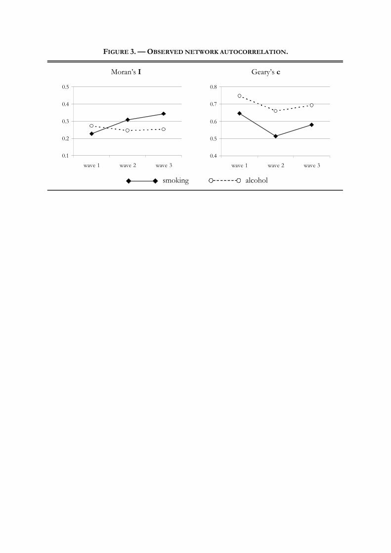
FIGURE 3. — OBSERVED NETWORK AUTOCORRELATION.

Moran’s I Geary’s c

0.1

0.2

0.3

0.4

0.5

wave 1 wave 2 wave 3

0.4

0.5

0.6

0.7

0.8

wave 1 wave 2 wave 3

smoking alcohol

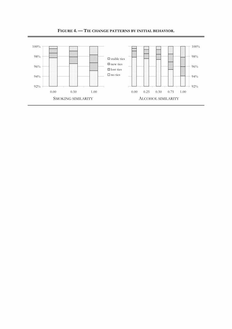
92%

94%

96%

98%

100%

0.00 0.50 1.00

stable ties

new ties

lost ties

no ties

92%

94%

96%

98%

100%

0.00 0.25 0.50 0.75 1.00

FIGURE 4. — TIE CHANGE PATTERNS BY INITIAL BEHAVIOR.

SMOKING SIMILARITY ALCOHOL SIMILARITY

0%

25%

50%

75%

100%

no tie tie

stay close

approach

distance

stay away

0%

25%

50%

75%

100%

no tie tie

FIGURE 5. — BEHAVIOR CHANGE PATTERNS BY INITIAL TIE STATUS.

SMOKING DYNAMICS ALCOHOL DYNAMICS

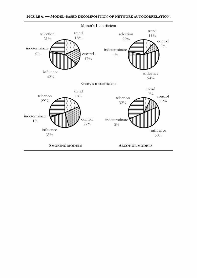
FIGURE 6. — MODEL-BASED DECOMPOSITION OF NETWORK AUTOCORRELATION.

Moran’s I-coefficient

Geary’s c-coefficient

SMOKING MODELS ALCOHOL MODELS

TABLE 1SCHEMATIC OVERVIEW OF THE MODEL COMPONENTS

occurrence rule of change

network changes . . . . . . . network rate function network objective function

behavioral changes . . . . . behavioral rate function behavioral objective function

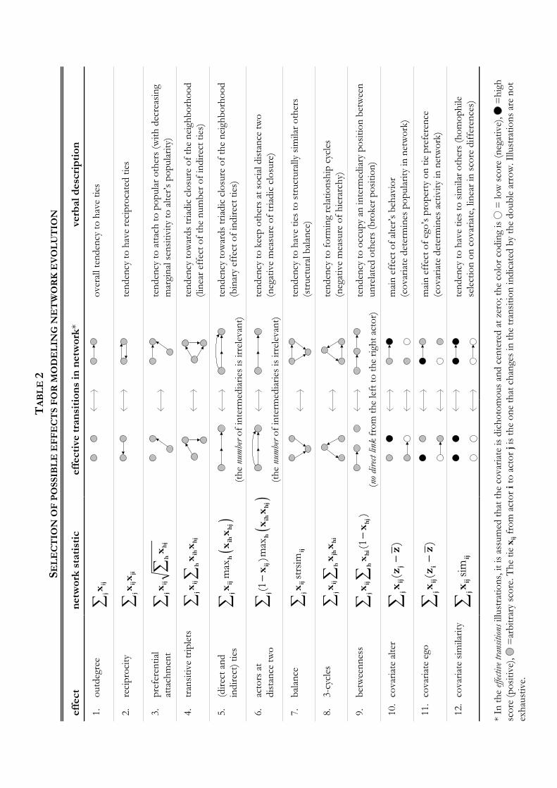
TABLE 2

SELECTIO

N O

F P

OSSIB

LE E

FFECTS F

OR M

ODELIN

G N

ETW

ORK E

VOLUTIO

N

effect

netw

ork

statistic

effective transitions in netw

ork*

verb

al desc

ription

1.

outdegree

∑ij

jx

overall tendency to have ties

2.

reciprocity

∑ij

jijx

xtendency to have reciprocated ties

3.

preferential

attachment

∑∑

ijhj

jh

xx

tendency to attach to popular others (w

ith decreasing

marginal sensitivity to alter’s popularity)

4.

transitive triplets

∑∑

ijih

hj

jh

xx

xtendency towards triadic closure of the neigh

borhood

(linear effect of the number of indirect ties)

5.

(direct and

indirect) ties

()

max

∑ij

hih

hj

jx

xx

tendency towards triadic closure of the neigh

borhood

(binary effect of indirect ties)

(the number of interm

ediaries is irrelevant)

6.

actors at

distance two

()

(1)m

ax−

∑ij

hih

hj

jx

xx

tendency to keep others at social distance two

(negative measure of triadic closure)

(the number of interm

ediaries is irrelevant)

7.

balance

strsim

∑ij

ijjx

tendency to have ties to structurally sim

ilar others

(structural balance)

8.

3-cycles

∑∑

ijjh

hi

jh

xx

xtendency to form

ing relationship cycles

(negative measure of hierarchy)

9.

betweenness

(1)

−∑

∑ij

hi

hj

jhx

xx

tendency to occupy an interm

ediary position between

unrelated others (broker position)

(no direct link from the left to the righ

t actor)

10.covariate alter

()

−∑

ijj

jx

zz

main effect of alter’s behavior

(covariate determines popularity in network)

11.covariate ego

()

−∑

iji

jx

zz

main effect of ego’s property on tie preference

(covariate determines activity in network)

12.covariate sim

ilarity

sim

∑ij

ijjx

tendency to have ties to sim

ilar others (homophile

selection on covariate, lin

ear in score differences)

* In the effective transitions illustrations, it is assumed that the covariate is dichotomous and centered at zero; the color coding is

= low score (negative),

=high

score (positive),

=arbitrary score. The tie x

ij from actor i to actor j is the one that changes in the transition indicated by the double arrow. Illustrations are not

exhaustive.

TABLE 3

SELECTIO

N OF POSSIB

LE N

ETWORK EFFECTS FOR M

ODELIN

G BEHAVIO

RAL EVOLUTIO

N

effect

network statistic

effective transitions in behavior*

verbal description

1.

shap

e: linear an

d

quad

ratic

and

()

−iz

z2

()

−iz

zThe two parameters together define a parabola shape of the

objective function, allowing to capture the basic shape of the

observed distribution of the behavioral variable.

2.

average

simila

rity

()

()

sim

ijij

ijj

jx

x∑

∑assimila

tion to neigh

bors’ av

erage beh

avior

(small neigh

borhoods pull as m

uch

as big ones)

3.

sum of simila

rity

sim

ijij

jx

∑assimila

tion to neigh

bors’ av

erage beh

avior

(size of neigh

borhood determines size of effect)

4.

average alters

()

()

()

−∑

∑ij

jij

jj

xz

zx

main effect of neigh

bors’ av

erage beh

avior

(contagion / influen

ce, but not necessarily assim

ilation)

5.

indeg

ree

× beh

avior

()

−∑

iji

jz

zx

effect of own popularity in the network on beh

avior

6.

outdeg

ree

× beh

avior

()

−∑

iij

jz

zx

effect of own activity in the network on beh

avior

7.

isolation

× beh

avior

()

(max

()

)1

−−

ij

jiz

xz

effect of being isolated in the network on beh

avior

* In the effective transitions illustrations, it is assumed

that the beh

avioral dep

enden

t variable is dichotomous an

d cen

tered at zero; the co

lor co

ding is

= low sco

re

(neg

ative),

=high sco

re (positive),

=arbitrary sco

re. A

ctor i is the actor who chan

ges co

lor zi in the tran

sition in

dicated

by the double arrows. Illu

strations are not

exhau

stive.

TABLE 4

SUMMARY OF EXPECTATIONS ABOUT MODEL PARAMETERS

Rules of network change (friendship)

verbal description model parameter sign

1. The density of friendship networks is low. outdegree –

2. Friendship nominations tends to be reciprocated. reciprocity +

3. Popular pupils attract friendship nominations. preferential attachment +

4. Friendship networks tend to display triadic closure.

(direct and indirect) ties +

distance-2 –

5. Friends tend to be structurally equivalent. balance +

6. Friendship is more likely between classmates. classmate +

7. There is homophily according to gender. gender similarity +

8. Older students are less invested in school networks. birth year ego/alter +

9. Money attracts friends. money alter +

10. There is homophily according to money. money similarity +

11. Romantic relations reduce investment in the network. romantic ego/alter –

12. There is homophily according to romantic relations. romantic similarity +

13. There is homophily according to substance use. behavior similarity +

Rules of behavioral change (substance use)

verbal description model parameter sign

14. Own substance use is assimilated to friends’ use. average similarity +

15. Older pupils use more substance. birth year –

16. Pupils whose parents/siblings smoke use more substance. parent/sibling smoking +

17. Pupils who use one substance also use the other. other substance use +

18. Pupils with more money use more substance. money +

19. Pupils involved in romantic relations use less substance. romantic –

NETW

ORK D

YN

AM

ICS

estimate

st.error

p-value

estimate

st.error

p-value

estimate

st.error

p-value

estimate

st.error

p-value

rate

period 1

16.73 (2.05)

16.23 (2.53)

11.29 (0.87)

6.51 (0.36)

rate

period 2

11.31

(1.38)

11.16

(1.06)

8.82 (0.85)

5.38

(0.28)

outd

egre

e (density

)-3.22

(0.17)

<0.001

-3.22

(0.16)

<0.001

-2.77 (0.06)

<0.001

-1.98

(0.03)

<0.001

recip

rocity

1.77

(0.10)

<0.001

1.81

(0.11)

<0.001

2.48 (0.09)

<0.001

—

pre

fere

ntial attachm

ent

0.35

(0.07)

<0.001

0.36

(0.07)

<0.001

—

—

(direct and indirect) tie

s0.68

(0.10)

<0.001

0.69

(0.10)

<0.001

—

—

num

ber of acto

rs a

t dista

nce 2

-0.32

(0.08)

<0.001

-0.35

(0.06)

<0.001

—

—

bala

nce

17.43

(3.77)

<0.001

16.24

(2.71)

<0.001

—

—

cla

ssm

ate

0.03

(0.07)

0.679

0.01

(0.08)

0.885

—

—

sex a

lter

-0.13

(0.09)

0.137

-0.15

0.08

0.068

—

—

sex e

go

0.09

(0.10)

0.375

0.09

0.12

0.492

—

—

sex sim

ilarity

0.65

(0.08)

<0.001

0.65

(0.08)

<0.001

0.96

(0.08)

<0.001

—

birth

year alter

0.14

(0.08)

0.074

0.15

(0.07)

0.039

—

—

birth

year ego

0.35

(0.10)

<0.001

0.36

(0.10)

<0.001

—

—

birth

year sim

ilarity

0.23

(0.14)

0.089

0.24

(0.17)

0.152

—

—

money a

lter

0.10

(0.05)

0.030

0.10

(0.05)

0.037

—

—

money e

go

-0.08

(0.07)

0.257

-0.05

(0.06)

0.372

—

—

money sim

ilarity

1.06

(0.28)

<0.001

1.07

(0.30)

<0.001

—

—

rom

antic a

lter

-0.01

(0.08)

0.912

-0.03

(0.08)

0.694

—

—

rom

antic e

go

-0.07

(0.10)

0.480

-0.09

(0.09)

0.353

—

—

rom

antic sim

ilarity

0.18

(0.08)

0.020

0.19

(0.07)

0.011

—

—

alc

ohol alter

0.005

(0.06)

0.936

—

—

—

alc

ohol ego

0.12

(0.09)

0.174

—

—

—

alc

ohol sim

ilarity

0.48

(0.42)

0.255

—

0.89

(0.47)

0.057

—

smokin

g a

lter

-0.02

(0.07)

0.822

—

—

—

smokin

g e

go

-0.05

(0.10)

0.586

—

—

—

smokin

g sim

ilarity

0.23

(0.16)

0.156

—

0.30

(0.12)

0.012

—

TABLE 5

full m

odel

c

ontrol m

odel

tre

nd m

odel

strawm

an m

odel

ESTIM

ATES A

ND

STAN

DARD

ERRO

RS F

OR F

RIE

ND

SH

IP E

VO

LU

TIO

N

ALCOHOL DYNAMICS

estimate

st.error

p-value

estimate

st.error

p-value

estimate

st.error

p-value

estimate

st.error

p-value

rate period 1

1.68

(0.32)

1.39

(0.24)

1.70

(0.32)

1.33

(0.20)

rate period 2

2.59

(0.57)

2.55

(0.69)

2.69

(0.63)

2.43

(0.49)

shape: linear

0.39

(0.36)

0.275

0.20

(0.26)

0.440

0.45

(0.18)

0.013

0.43

(0.11)

<0.001

shape: quadratic

0.02

(0.11)

0.830

-0.31

(0.07)

<0.001

0.07

(0.12)

0.545

-0.28

(0.06)

<0.001

average sim

ilarity

6.94

(2.06)

<0.001

—

7.42

(2.52)

0.003

—

smoking

0.04

(0.19)

0.824

0.15

(0.16)

0.360

—

—

sex

0.04

(0.25)

0.869

0.13

(0.20)

0.496

-0.06

(0.22)

0.795

—

birth year

0.29

(0.30)

0.330

0.14

(0.24)

0.561

—

—

money

0.20

(0.18)

0.268

0.19

(0.12)

0.111

—

—

romantic

-0.45

(0.33)

0.177

-0.23

(0.25)

0.354

—

—

SMOKIN

G DYNAMICS

estimate

st.error

p-value

estimate

st.error

p-value

estimate

st.error

p-value

estimate

st.error

p-value

rate period 1

5.20

(1.87)

4.54

(1.59)

4.94

(1.62)

3.95

(0.99)

rate period 2

4.26

(1.75)

4.64

(2.98)

3.94

(1.40)

4.21

(0.94)

shape: linear

-2.64

(0.38)

<0.001

-3.39

(0.46)

<0.001

-2.55

(0.58)

<0.001

-3.44

(0.33)

<0.001

shape: quadratic

2.63

(0.32)

<0.001

2.70

(0.40)

<0.001

2.69

(0.37)

<0.001

2.82

(0.28)

<0.001

average sim

ilarity

2.63

(1.08)

0.015

—

2.92

(1.24)

0.018

—

alcohol

0.004

(0.19)

0.983

0.06

(0.17)

0.739

—

—

sex

-0.003

(0.27)

0.990

0.24

(0.21)

0.260

-0.05

(0.29)

0.866

—

birth year

0.04

(0.32)

0.910

-0.11

(0.24)

0.651

—

—

parent sm

oking

-0.26

(0.29)

0.373

-0.16

(0.23)

0.483

—

—

sibling smoking

0.24

(0.37)

0.520

0.15

(0.35)

0.659

—

—

money

0.05

(0.20)

0.789

0.10

(0.14)

0.488

—

—

romantic

0.22

(0.28)

0.435

0.27

(0.29)

0.366

—

—

full m

odel

control model

trend m

odel

ESTIM

ATES AND STANDARD ERRORS FOR THE EVOLUTIO

N OF SUBSTANCE USE

strawman m

odel

TABLE 6

strawman m

odel

full m

odel

control model

trend m

odel

TABLE 7. — MODEL-BASED SIMULATED NETWORK AUTOCORRELATION.

SMOKING ALCOHOL

model Moran Geary model Moran Geary

null -0.006 1.000 null -0.006 1.000

trend 0.044 (0.036) 0.928 (0.048) trend 0.026 (0.041) 0.977 (0.053)

control 0.092 (0.046) 0.822 (0.063) control 0.052 (0.052) 0.941 (0.066)

no influence 0.150 (0.048) 0.704 (0.063) no influence 0.115 (0.050) 0.840 (0.062)

no selection 0.204 (0.056) 0.722 (0.061) no selection 0.209 (0.061) 0.782 (0.061)

full 0.268 (0.056) 0.608 (0.060) full 0.283 (0.060) 0.681 (0.057)

observed 0.327 0.546 observed 0.250 0.677