Lecture #3What can go wrong?

Trajectories of hybrid systems

João P. Hespanha

University of Californiaat Santa Barbara

Hybrid Control and Switched Systems

Summary

1. Trajectories of hybrid systems:• Solution to a hybrid system• Execution of a hybrid system

2. Degeneracies• Finite escape time• Chattering• Zeno trajectories• Non-continuous dependency on initial conditions

Hybrid Automaton (deterministic)

Q ´ set of discrete states Rn ´ continuous state-spacef : Q £ Rn ! Rn ´ vector field : Q £ Rn ! Q ´ discrete transition : Q £ Rn ! Rn ´ reset map

mode q1 mode q3

(q1,x–) = q3 ?

mode q2

(q1,x–) = q2 ?x(q1,x–)

x(q1,x–)

Hybrid Automaton

Q ´ set of discrete states Rn ´ continuous state-spacef : Q £ Rn ! Rn ´ vector field : Q £ Rn ! Q £ Rn ´ discrete transition (& reset map)

mode q1 mode q3

1(q1,x–) = q3 ?

mode q2

1(q1,x–) = q2 ?x2(q1,x–)

x2(q1,x–)

Compact representation of a hybrid automaton

Definition: A solution to the hybrid automaton is a pair of right-continuous signals x : [0,1) ! Rn q : [0,1) ! Q

such that

1. x is piecewise differentiable & q is piecewise constant

2. on any interval (t1,t2) on which q is constant and x continuous

3.

Solution to a hybrid automaton

mode q1mode q2

1(q1,x–) = q2 ?x2(q1,x–)

continuous evolution

discrete transitions

Example #4: Inverted pendulum swing-up

u 2 [-1,1] Hybrid controller:

1st pump/remove energy into/from the system by applying maximum force, until E ¼ 0

2nd wait until pendulum is close to the upright position

3th next to upright position use feedback linearization controller

pump energy

remove energy

wait stabilize

E 2 [–,] ?

E 2 [–,] ?

E>

E < –

+ || ·

Example #4: Inverted pendulum swing-up

pump energy wait stabilize

+ || ·

Q = { pump, wait, stab } R2 = continuous state-space

¸ –

Example #4: Inverted pendulum swing-up

pump energy wait stabilize

+ || ·

Q = { pump, wait, stab } R2 = continuous state-space

¸ –

What if we already have + || · when E reaches –

–

E

+ ||

q = pump

q = wait q = stab

t

Example #4: Inverted pendulum swing-up

pump energy wait stabilize

+ || ·

Q = { pump, wait, stab } R2 = continuous state-space

¸ –

–

E

+ ||

q = pump

q = wait

q = stabt

t*

q( t* ) = ?

In general, we may need more than one value for the state at each instant of time

Hybrid signals

Definition: A hybrid time trajectory is a (finite or infinite) sequence of closed intervals = { [i,'i] : i · 'i, 'i = i+1 , i =1,2, … }

(if is finite the last interval may by open on the right)T ´ set of hybrid time trajectories

Definition: For a given = { [i,'i] : i · 'i, i+1 = 'i, i =1,2, … } 2 Ta hybrid signal defined on with values on X is a sequence of functions

x = {xi : [i,'i]!X i =1,2, … } x : ! X ´ hybrid signal defined on with values on X

[,] [,]

[,1)

t

E.g., › { [0,1], [1,1], [1,1], [1,+1) }, x › { t/2 , 1/4 , 3/4, 1/t }

t/2 1/4

1/t3/4

[,]

A hybrid signal can take multiple values for the same time-instant

Execution of a hybrid automaton

Definition: An execution of the hybrid automaton is a pair of hybrid signals x : ! Rn q : ! Q { [i,'i] : i =1,2, … } 2 T

such that

1. on any [i,'i] 2 qi is constant and

2.

mode q1mode q2

1(q1,x–) = q2 ?x2(q1,x–)

continuous evolution

discrete transitions

Example #4: Inverted pendulum swing-up

pump energy wait stabilize

+ || ·

Q = { pump, wait, stab } R2 = continuous state-space

¸ –

–

E

+ ||

q = pump

q = wait

q = stab

t*

t

{ [0,t*], [t*, t*], [t*,+1) }q { pump , wait , stab }x { … , … , … }

1. There are other concepts of solution that also avoid this problem [Teel 2005]

2. Could one “fix” this hybrid system to still work with the usual notion of solution?

What can go wrong?

1. Problems in the continuous evolution :• existence• uniqueness• finite escape

2. Problems in the hybrid execution:• Chattering• Zeno

3. Non-continuous dependency on initial conditions

Existence

Theorem [Existence of solution]

If f : Rn ! Rn is continuous, then 8 x0 2 Rn there exists at least one solution with x(0) = x0, defined on some interval [0,)

There is no solution to this differential equation that starts with x(0) = 0

x

f(x)

Why? one any interval [0,) x cannot: remain zero, become positive, or become negative.

discontinuous

(x = 0 would make some sense)

Uniqueness

x

f(x)

There are multiple solutions that start at x(0) = 0, e.g.,

t

x

t

Theorem [Uniqueness of solution]

If f : Rn ! Rn is Lipschitz continuous, then 8 x0 2 Rn there a single solution with x(0) = x0, defined on some interval [0,)

1 derivative at 0

Definitions: A function f : Rn ! Rn is Lipschitz continuous if in any bounded subset of S of Rn there exists a constant c such that

(f is differentiable almost everywhere and the derivative is bounded on any bounded set)

Finite escape time

Any solution that does not start at x(0) = 0 is of the form

T

T-1

finite escape ´ solution x tends to 1 in finite time

Definitions: A function f : Rn ! Rn is globally Lipschitz continuous if there exists a constant c such that

f grows no faster than linearly

Theorem [Uniqueness of solution]

If f : Rn ! Rn is globally Lipschitz continuous, then 8 x0 2 Rn there a single solution with x(0) = x0, defined on [0,1)

x

t

unbounded derivative

Degenerate executions due to problems in the continuous evolution

q = 1 q = 2

x ¸ 1 ? = { [0,1] , [1,2] }q = {q1(t) = 1 , q2(t) = 2 }x = {x1(t) = t , x2(t) = 2 – t }

x

t

x1(t) x2(t)

q = 1 q = 2

x ¸ 1 ?

1 2

= { [0,1] , [1,2) }q = {q1(t) = 1 , q2(t) = 2 }x = {x1(t) = t , x2(t) = 1/(2 – t) }

x

t

x1(t)

x2(t)

1 2

Chattering

q = 2x ¸ 0 ?

x < 0 ?

q = 1

There is no solution past x = 0

t

x (t)

1

but there is an execution

= { [0,1] , [1], [1], [1], … }q = {q1(t) = 2 , q2(t) = 1, q1(t) = 2, …}x = {x1(t) = 1 – t , x2(t) = 0, x2(t) = 0, …}

Chattering execution ´ is infinite but after some time, all intervals are singletons

t

x1 (t)

1

xk (t) k¸ 2

q1 (t) q2k+1 (t) k¸ 1

q2k (t) k¸ 1

Example #3: Semi-automatic transmission

g = 1 g = 2 g = 3 g = 4

v(t) 2 { up, down, keep } ´ drivers input (discrete)

v = up or ¸ 2 ? v = up or ¸ 3 ? v = up or ¸ 4 ?

v = down or · 1 ? v = down or · 2 ? v = down or · 3 ?

2

3

4

1

2

3

g = 1

g = 2g = 3

g = 4

If the driver sets v(t) = up 8 t ¸ t* and t · 1 one gets chattering. For ever?

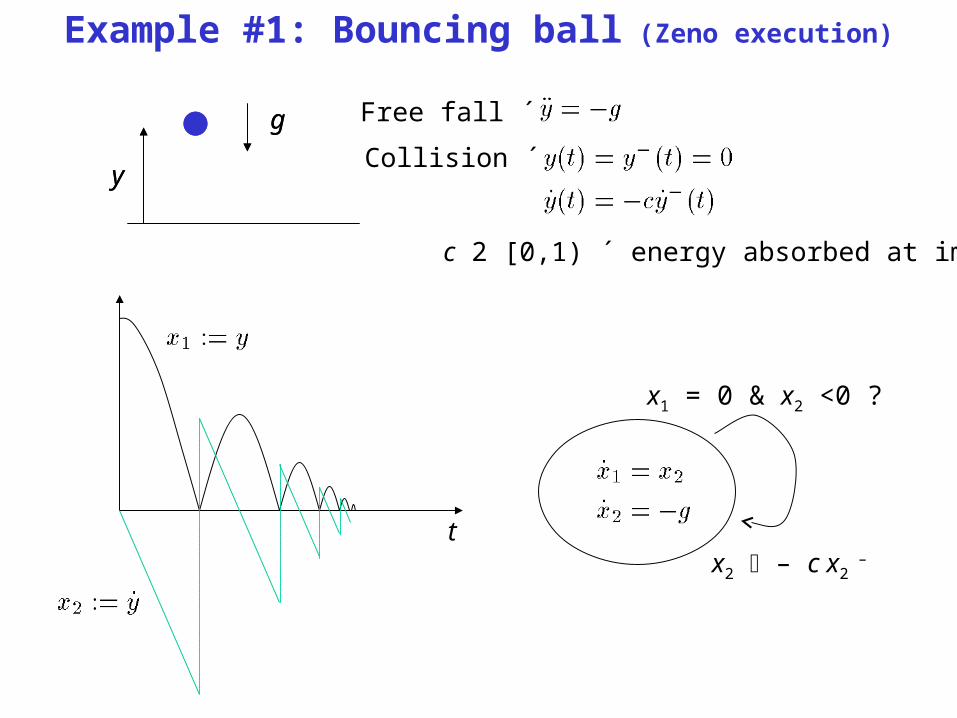
Example #1: Bouncing ball (Zeno execution)

t

Free fall ´

Collision ´g

y

g

y

c 2 [0,1) ´ energy absorbed at impact

x1 = 0 & x2 <0 ?

x2 – c x2 –

Zeno solution

tt1 t2 t3

x1 = 0 & x2 <0 ?

x2 – c x2 –

Zeno execution

tt1 t2 t3

Zeno execution ´ is infinite but the execution does not extend to t = +1

Zeno time´1 › sups2 s

x1 = 0 & x2 <0 ?

x2 – c x2 –

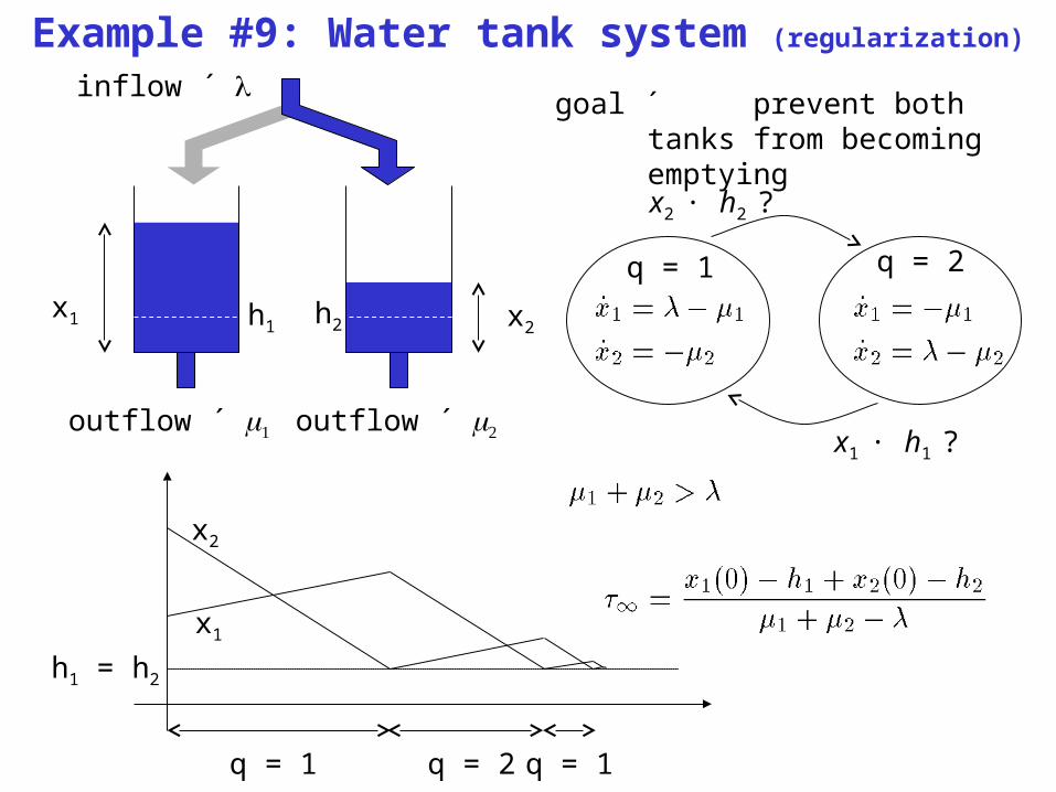
Example #9: Water tank system (regularization)

x2

goal ´ prevent both tanks from becoming emptying

outflow ´

inflow ´

x1

outflow ´

h1 h2

q = 1

q = 2

x2 · h2 ?

x1 · h1 ?

x1

x2

q = 2 q = 1

q = 1

h1 = h2

Temporal regularizationExample #9: Water tank system

x2

outflow ´

inflow ´

x1

outflow ´

h1 h2

q = 2

x2 · h2 ?

x1 · h1 ?

only jump after a minimum time has elapsed

q = 2

x2 · h2, > ?

x1 · h1, > ?

› 0

› 0

q = 1

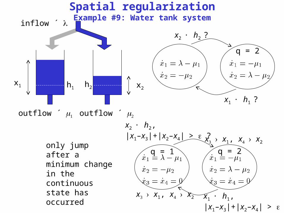
Spatial regularizationExample #9: Water tank system

x2

outflow ´

inflow ´

x1

outflow ´

h1 h2

q = 2

x2 · h2 ?

x1 · h1 ?

q = 2

x2 · h2,|x1–x3|+|x2–x4|> ? x› x1, x› x2

q = 1

x› x1, x› x2 x1 · h1,|x1–x3|+|x2–x4|> ?

only jump after a minimum change in the continuous state has occurred

Continuity with respect to initial conditions

Theorem [Uniqueness & continuity of solution]

If f : Rn ! Rn is Lipschitz continuous, then 8 x0 2 Rn there a single solution with x(0) = x0, defined on some interval [0,)

Moreover, given any T < 1, and two solutions x1, x2 that exist on [0,T]:

8> 0 9> 0 : ||x1(0) – x2(0)|| · ) ||x1(t) – x2(t)|| · 8 t 2 [0,T]

value of the solution on the interval [0,T] is continuous with respect to the initial conditions

Discontinuity with respect to initial conditions

x1 ¸ 0 & x2 > 0 ? mode q1x1 ¸ 0 & x2 · 0 ?

x1

x2

– 1 x1

x2

1

no matter how close to zero x2(0) = > 0 is, x2(2) = – 1

if x2(0) = 0 then x2(2) = 1

mode q2 mode q3

problem arises from discontinuity of the transition function

Next class…

1. Numerical simulation of hybrid automata• simulations of ODEs• zero-crossing detection

2. Simulators• Simulink• Stateflow• SHIFT• Modelica

Follow-up homework• Find conditions for the existence of solution to a hybrid system