Buoyant force

Vg

BF

The volume of gas (liquid) is at rest with respect to its surrounding gas (liquid): the force of gravity is balanced by the buoyant force APPF topbottomB )(

bottomP

topP

P

h

bottomPtopP

Note that the buoyant force does not care what’s inside this volume (a brick, a gas, or vacuum): it depends only on the volume and the density of the outside gas (liquid).

Lecture 3. Transport Phenomena (Ch.1)Lecture 2 – various processes in macro systems near the state of equilibrium can be described by a handful of macro parameters. Quasi-static processes – sufficiently slow processes, at any moment the system is almost in equilibrium.

It is important to know how much time it takes for a system to approach an equilibrium state. A system is not in equilibrium when the macroscopic parameters (T, P, etc.) are not constant throughout the system. To approach equilibrium, these non-uniformities have to be ironed out through the transport of energy, momentum, and mass from one part of the system to another. The mechanism of transport is molecular collisions. Our goal - to estimate the characteristic rates of approaching equilibrium, and, thus, to impose limitations on the rates of “quasi-static” processes.

1. Transfers of Q (“Heat” Conduction)

2. Transfers of Mass (Diffusion)

One-dimensional (1D) case:

x

n(x,t)T(x,t)

The Mean Free Path of MoleculesTransports energy, momentum, mass – due to random thermal motion of molecules in gases and liquids.

An estimate: one molecule is moving with a constant speed v, the other molecules are fixed. Model of hard spheres, the radius of molecule r ~ 110-10 m.

4r

The av. distance traversed by a molecule until the 1st collision is the distance in which the av. # of molecules in this cylinder is 1.

12 2 VNlr

nNV

rl

1

41

2 n

l21

Maxwell:

The mean free path l - the average distance traveled by a molecule btw two successive collisions.

The average time interval between successive collisions - the collision time:

vl

- the most probable speed of a moleculev

l

n = N/V – the density of molecules = 4r2 – the cross section

Some Numbers:

3265

23

m104Pa10

K300J/K1038.11

PTk

NV

nBair at norm. conditions:

P = 105 Pa: l ~ 10-7 m - 30 times greater than d

P = 10-2 Pa (10-4mbar): l ~ 1 m (size of a typical vacuum chamber)

- at this P, there are still ~2.5 1012 molecule/cm3 (!)

m 103~ 93 NVd

3/23/2 Pndl

The collision time at norm. conditions: ~ 10-7m / 500m/s = 2·10-10 s

For H2 gas in interstellar space, where the density is ~ 1 molecule/ cm3,

l ~ 1013 m - ~ 100 times greater than the Sun-Earth distance (1.5 1011 m)

for an ideal gas: TnkPTNkPV BB PT

nl

1n

l

1

the intermol. distance

Transport in Gases (Liquids)Box 1 Box 2

l

Simplified approach: consider the “ballistic” molecule exchange between two “boxes” within the gas (thickness of each box should be comparable to the mean free path of molecules, l). During the average time between molecular collisions, , roughly half the molecules in Box 1 will move to the right in Box 2, while roughly half the molecules in Box 2 will move to the left in Box 1.

Each molecule “carries” some quantity (mass, kin. energy, etc.), within each box - = N = A l n . E.g., the flux of the number of molecules across the border per unit area of the border, Jx:

xnD

xnlv

xnlvlxnlxnv

tANJ n

312

61

61

x=-l

in a 3D case, on average 1/6 of the molecules have a velocity along +x or –x

“-” - if n/x is negative, the flux is in the positive x direction (the current flows from high density to low density)

x=0 x=l

xn(x,t) Jx

In a 3D case, TKJnDJ thUn

the diffusion constant

Diffusion

Diffusion – the flow of randomly moving particles caused by variations of the concentration of particles. Example: a mixture of two gases, the total concentration n = n1+n2 =const over the volume (P = const).

J J

Fick’s Law:

n1 n2

xnD

xnvlJ x

31 vlD

31

- the diffusion coefficient(numerical pre-factor depends on the dimensionality: 3D – 1/3; 2D – 1/2)

vlD31

its dimensions [L]2 [t]-1, its units m2 s-1

Typically, at normal conditions, l ~10-7 m, v ~300 m/s D ~ 10-5 m2 s-1

(in liquids, D is much smaller, ~10-10 m2 s-1)

For electrons in well-ordered semiconductor heterostructures at low T:l ~10-5 m, v ~105 m/s D ~ 1 m2 s-1

Diffusion Coefficient of an Ideal Gas ( Pr. 1.70 )

for an ideal gas:PTk

nl B

1

from the equipartition theorem: 2/1Tv PT

PTTD

2/32/1

therefore, at a const. temperature:P

D 1

and at a const. pressure: 2/3TD

The Diffusion Equation

n(x,t) tAxJ x

flow in

tAxxJ x

flow out

x x+x

xJ

tn x

change of n inside:

xnDJ x

combining with

we’ll get the equation that describes one-dimensional diffusion:

2

2

xnD

tn

the solution which corresponds to an initial condition that all particles are at x =0 at t =0:

Dtx

DtCtxn

4exp,

2

C is a normalization factor

the rms displacement of particles: Dtx 2

the diffusion equation

t1 =0

x =0

t2 =t

Brownian Motion (self-diffusion)

The experiment by the botanist R. Brown concerning the drifting of tiny (~ 1m) specks in liquids and gases, had been known since 1827.Brownian motion was in focus of the struggle for and against the atomic structure of matter, which went on during the second half of the 19th century and involved many prominent physicists.

Ernst Mach: “If the belief in the existence of atoms is so crucial in your eyes, I hereby withdraw from the physicist’s way of thought...”

Albert Einstein explained the phenomenon on the basis of the kinetic theory (1905), connected in a quantitative manner the Brownian motion and such macroscopic quantities as the coefficients of mobility and viscosity – and brought the debate to a conclusion in a short time.

Observing the Brownian motion under a microscope, Jean Perrin measured the Boltzman constant and Avogadro number in 1908 (Nobel 1926).

Historical background:

Brownian Motion(cont.) tDx

t

2

a 1D random walk of a drunk

t

xGaussian distribution

For air at normal conditions , it takes )/sm107.1m/s500m10( 257 Dvlfor a molecule to “diffuse” over 1m: odor spreads by convections10~ 5

2

DLt

the rms displacement

For electrons in metals at 300K , it takes )/sm103m/s10m10( 2267 Dvlto “diffuse” over 1m. For the electron gas in metals, convection can be ignored: the electron velocities are randomized by impurity/phonon scattering.

s30~2

DLt

A body that participates in a random walk, or a subject of random collisions with the gas molecules. Its average displacement is zero. However, the average square distance grows linearly with time:

after N steps, the position is nlRR NN

111NR n - a randomly

oriented unit vector

01 NR

NNNN RnllRnlRR

222221

after averaging ( ): 2221 lRR NN

tlNRN 22

Dtx

DtCtxn

4exp,

2

Static Energy Flow by “Heat” Conduction

T1 T2

x

area A Heat conduction ( static heat flow, T = const)

xTKJ

xT

CK

xJ

CtT

thUthU

2

21In general, the energy transport due to molecular motion is described by the equation of heat conduction:

Thus, in principle, if you know the initial conditions, e.g. T(x,t=t0), you can describe the process by solving the equation. Often, you are asked to consider a different situation: a static flow of energy from a “hot” object to a “cold” one. (At what rate the internal energy is transferred between two systems with T1 T2 or between parts of a non-equilibrium system (if one can introduce Ti) ?) The temperature distribution in this formulation is time-independent, and we need to calculate the flux of thermal energy JU due to the heat conduction (diffusion/intermixing of particles with different energies, interactions between the particles that vibrate but do not move “translationally”).

T(x)T1

T2x

JU

Fourier Heat Conduction Law

T1 T2

x

AKGTGJ thU ,power

G – the thermal conductivity [W/K]R =1/G – the thermal resistivity

Electricity Thermal Physics

Charge Q Th. Energy, Q

Currant dQ/dt Power Q/dt

What “flows”

Flux

Driving “force”El.-stat. pot. difference

Temperature difference

“Resistance” El. resistance R Th. resistance R

Connection in series (Pr. 1.57):

Rtot = R1 + R2

Connection in parallel:Rtot

-1 = R1-1 + R2

-1

T1 T2

T1 T2

G

Ax

tTQ

Kth [W/K·m] – the thermal conductivity (material-specific)

xTAK

tQJ thU

For a window glass (Kth =0.8W/mK, 3 mm thick, A=1m2) and T = 20K:

Wm

KmKW/m 5300003.020)1)(8.0( 2

tQ

“-” - if T increases from left to right, energy flows from right to left

~ 10 times greater than in reality, a thin layer of still air

must contribute to thermal insulation.

Pr. 1.56

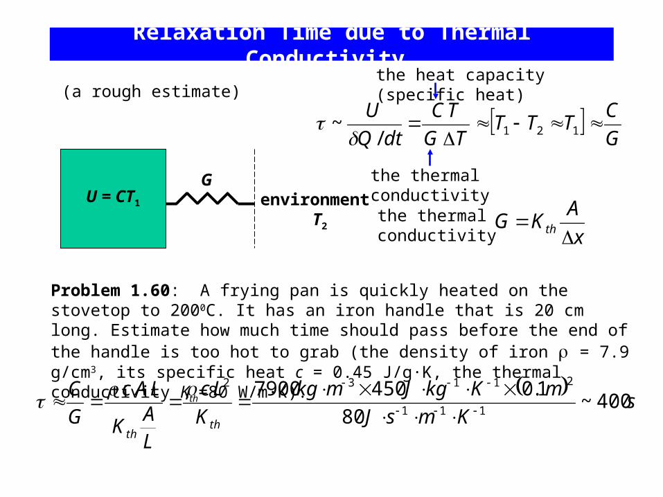
Relaxation Time due to Thermal Conductivity

(a rough estimate)

U = CT1

Genvironment

T2

GCTTT

TGTC

dtQU

121/~

Problem 1.60: A frying pan is quickly heated on the stovetop to 2000C. It has an iron handle that is 20 cm long. Estimate how much time should pass before the end of the handle is too hot to grab (the density of iron = 7.9 g/cm3, its specific heat c = 0.45 J/g·K, the thermal conductivity Kth=80 W/m·K).

xAKG th

sKmsJ

mKkgJmkgK

Lc

LAK

LAcGC

thth

400~80

1.04507900111

21132

the thermalconductivity

the thermal conductivity

the heat capacity (specific heat)

Thermal Conductivity of an Ideal Gas

Box 1 Box 2

T

dxdTvC

dxdTlCTTCUUQ

VVV

21

21

21

21 2121

lxTAKQ

th

vl

VC

lAvlC

AvCK VVV

th 21

21

21

B

BV

V knfV

Nkf

VCc

22

vlknfK Bth 4

Energy “flow”, t ~ :

KmW0.02500m/smJ/Km

723325 101038.1104.245

4vlknfK Bth

the specific heat capacity

(exp. value – 0.026 W/m·K)

The thermal conductivity of air at norm. conditions:

T1 T2

the time between two consecutive collisions v

l

Thermal Conductivity of Gases (cont.)

2. Thermal conductivity of an ideal gas is independent of the gas density!

This conclusion holds only if L >> l . For L < l , Kth n

Dewar

mTK

mTvnlvlknfK thBht ,

41

1.

mK th /1

- an argon-filled window helps to reduce Q

(at higher densities, more molecules participate in the energy transfer, but they carry the energy over a shorter distance)

Sate-of-the-art Bolometers (direct detectors of e.-m. radiation)

Ti

Nb

0.1 1104

105

106

107

108

109

HEDDs meanders

G, W

/Km3

T, K

Ge-ph= Ce/e-ph

G = Cph/es

electrons

phonons

heat sink

ħ

Te

T

Tphphe

phe GG

~

VTc Ge ph

1

10

100

1000

10 100 1000

BT85-4

BT87-1

BT100-1

BT121-1

BT121-4

Tim

e co

nsta

nt (

µs)

Temperature (mK)

phephephe TTTGTTGRIdtQ

2power

specific heat of electrons

Momentum Transfer, Viscosity

uxz

Drag – transfer of the momentum in the direction perpendicular to velocity.

Laminar flow of a gas (fluid) between two surfaces moving with respect to each other.

z

bottom,top,

xx

xx

uuAF

tp

zud

AF xx

Fx – the viscous drag force, - the coefficient of viscosity

Fx/A – shear stress

Viscosity of an ideal gas ( Pr. 1.66 ):Box 2

Box 1z ~ l

ux (z2)

ux (z1) xxxz uNmzNmuzNmup

21)(

21)(

21

21

zddulv

AF

lAvuNmp

AAF xxxzx

21

21

lv21

T1/2

Effusion of an Ideal Gas- the process of a gas escaping through a small hole (a << l) into a vacuum (Pr. 1.22) – the collisionless regime.

The opposite limit of a very large hole ( a >> l ) – the hydrodynamic regime.

The number of molecules that escape through a hole of area A in 1 sec, Nh, in terms of P(t ), T (how is T changing in the process?)

Atvm

NAt

pNP xhh

121

x

h vmtAPN

2

mTkvvTkvmv B

xxBxx 22 ,21

21

Nh = - N, where N is the total # of molecules in a system

mTk

VtAN

Tkm

mtA

VTNk

Tkm

mtAPN B

B

B

B 222

NNmTk

VA

tN B

1

2

Tkm

AVtNtN

B

2,exp)0()(

Depressurizing of a space ship, V - 50m3, A of a hole in a wall – 10-4 m2

(clearly, a << l does not apply)s3000s3.01010

K30J/K1038.1kg107.130

m10m502 26

23

27

24

3