Lecture 3 The energy equation - skeddanblog · PDF fileENG2038M – Fluid Mechanics 2 Lecture 2 recap Flow Classifications • Conditions in a body of fluid can vary from point to

ENG2038M – Fluid Mechanics 2

Lecture 3The energy equation

Dr Tim Gough: [email protected]


General information

• Lab groups now assigned

• Timetable up to week 6 published

• Is there anyone not yet on the list?

• Can anyone not see Blackboard yet?

• Please see me at interval and I’ll sort this out.

Week 3 Week 4 Week 5 Week 6

Tuesday 14.00 - 17.00 01 October 2013 08 October 2013 15 October 2013 22 October 2013Friday 14.00 - 17.00 04 October 2013 11 October 2013 18 October 2013 25 October 2013

Dr Tim GoughENG 2038 M 2 J1 2 J2

Fluid Mechanics 2Chesham Building C.01.14

18 18 18


Lecture 2 recap

• Streamlines etc

• Flow classifications

• Viscous and inviscid flows

• Discharge and mean velocity

• Flow continuity

• Flow continuity problems


Lecture 2 recap

Flow Classifications

• Conditions in a body of fluid can vary from point to point and, at any given point, can vary from one moment of time to the next.

• Flow is described as uniform if the velocity at a given instant is the same in magnitude and direction at every point in the fluid.

• If, at a given instant, the velocity changes from point to point, the flow is described as non‐uniform.

• A steady flow is one in which the velocity, pressure and cross‐section of the stream may vary from point to point but do not vary with time.

• If, at any given point, conditions do change with time, the flow is described as unsteady.


Lecture 2 recap

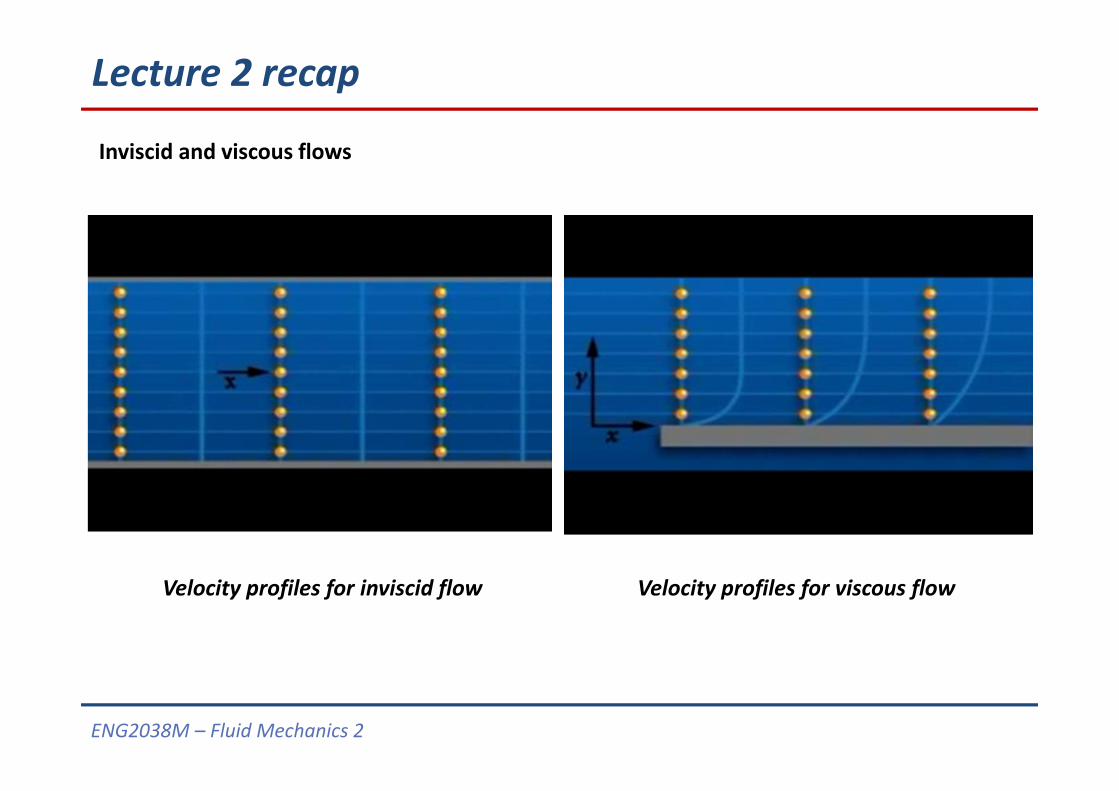
Inviscid and viscous flows

Velocity profiles for viscous flowVelocity profiles for inviscid flow


Lecture 2 recap

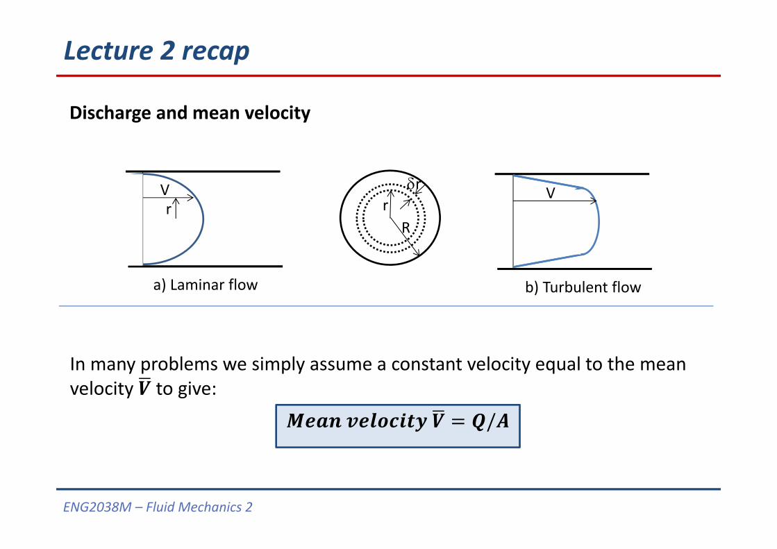
Discharge and mean velocity

/

In many problems we simply assume a constant velocity equal to the mean velocity to give:

b) Turbulent flow

Vrr

R

Vr

a) Laminar flow


12

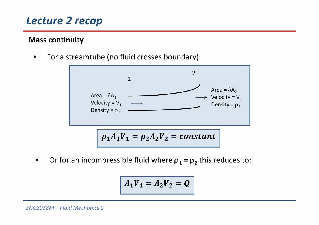
Area = A1Velocity = V1Density = 1

Area = A2Velocity = V2Density = 2

• For a streamtube (no fluid crosses boundary):

Lecture 2 recapMass continuity

• Or for an incompressible fluid where 1 = 2 this reduces to:


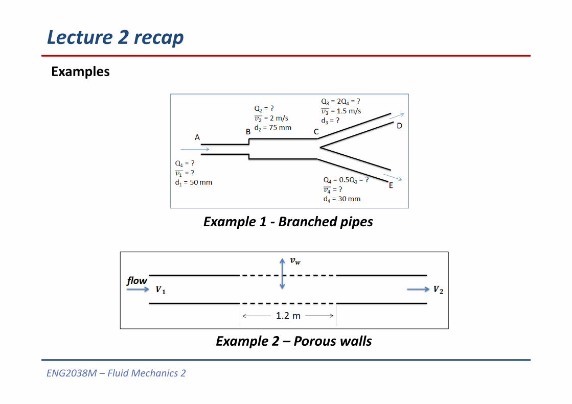
Lecture 2 recapExamples

Example 1 ‐ Branched pipes

Example 2 – Porous walls


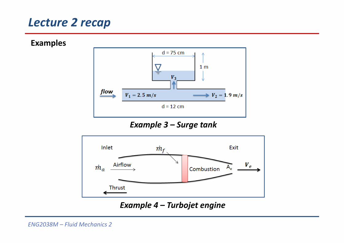
Lecture 2 recapExamples

Example 3 – Surge tank

Example 4 – Turbojet engine


The energy equation


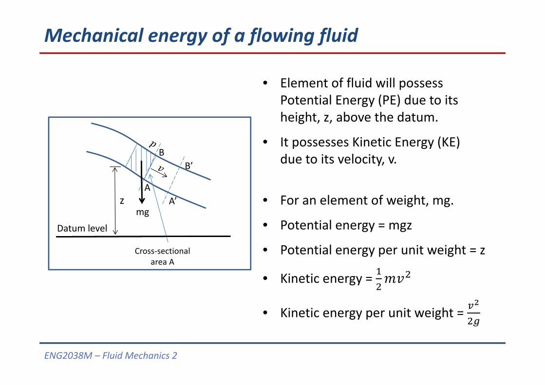
Mechanical energy of a flowing fluid

• Element of fluid will possess Potential Energy (PE) due to its height, z, above the datum.

• It possesses Kinetic Energy (KE) due to its velocity, v.

• For an element of weight, mg.

• Potential energy = mgz

• Potential energy per unit weight = z

• Kinetic energy =

• Kinetic energy per unit weight =

A

B

A’

B’

mg

Cross‐sectional area A

z

Datum level


A

B

A’

B’

Datum level

mg


z

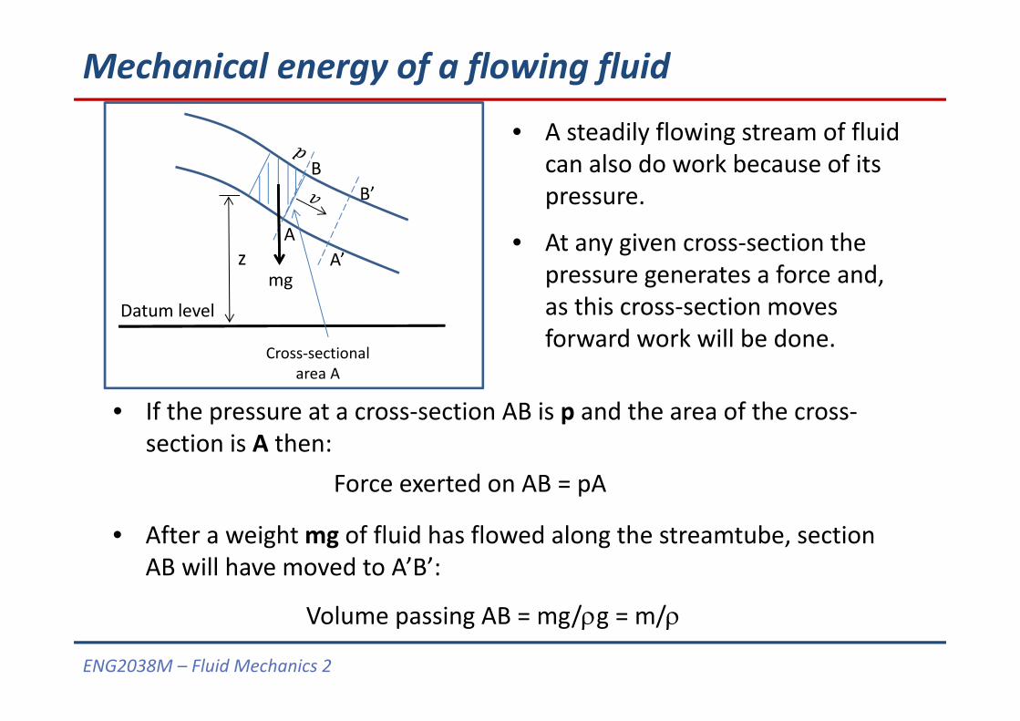
• A steadily flowing stream of fluid can also do work because of its pressure.

• At any given cross‐section the pressure generates a force and, as this cross‐section moves forward work will be done.

• If the pressure at a cross‐section AB is p and the area of the cross‐section is A then:

Force exerted on AB = pA

• After a weight mg of fluid has flowed along the streamtube, section AB will have moved to A’B’:

Volume passing AB = mg/g = m/




A

B

A’

B’

Datum level

mg


z

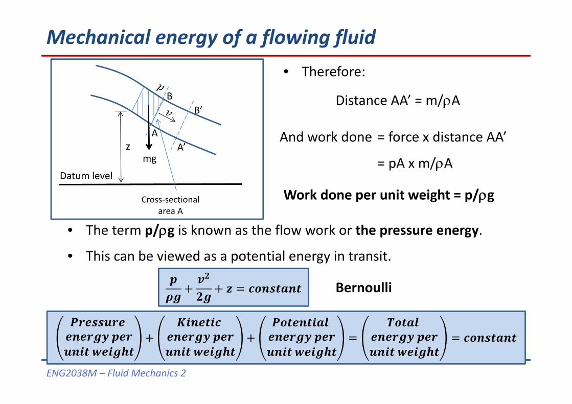
• Therefore:

Distance AA’ = m/A

And work done = force x distance AA’

= pA x m/A

Work done per unit weight = p/g

• The term p/g is known as the flow work or the pressure energy.

• This can be viewed as a potential energy in transit.

Bernoulli



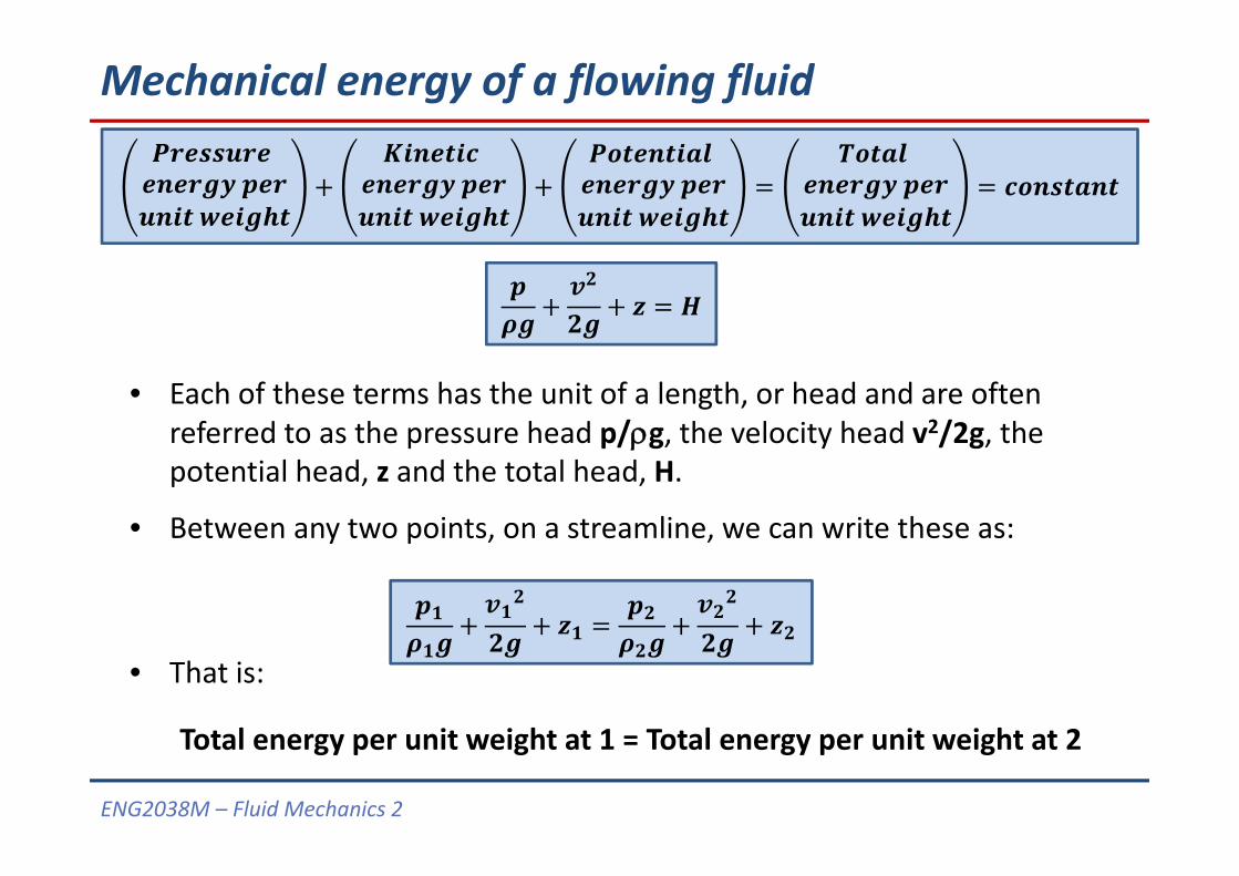
• Each of these terms has the unit of a length, or head and are often referred to as the pressure head p/g, the velocity head v2/2g, the potential head, z and the total head, H.

• Between any two points, on a streamline, we can write these as:

• That is:

Total energy per unit weight at 1 = Total energy per unit weight at 2



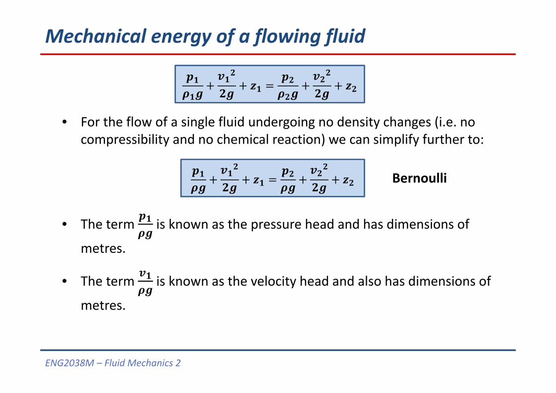
• For the flow of a single fluid undergoing no density changes (i.e. no compressibility and no chemical reaction) we can simplify further to:

Bernoulli

• The term is known as the pressure head and has dimensions of

metres.

• The term is known as the velocity head and also has dimensions of

metres.


Bernoulli's theorem

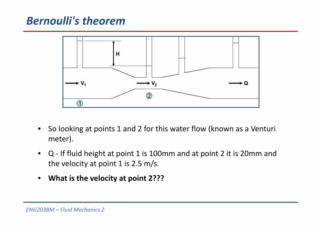
• So looking at points 1 and 2 for this water flow (known as a Venturimeter).

• Q ‐ If fluid height at point 1 is 100mm and at point 2 it is 20mm and the velocity at point 1 is 2.5 m/s.

• What is the velocity at point 2???


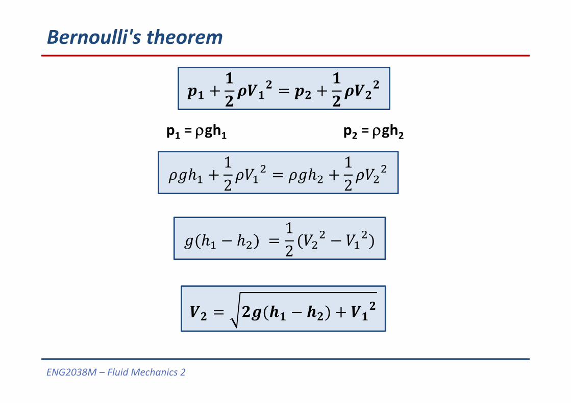
Bernoulli's theorem

p1 = gh1 p2 = gh2

12

12

12


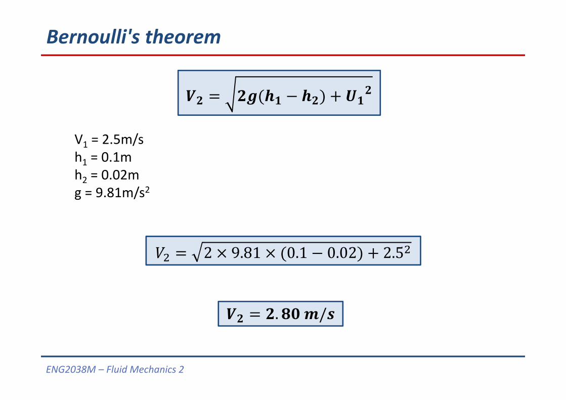
Bernoulli's theorem

V1 = 2.5m/sh1 = 0.1mh2 = 0.02mg = 9.81m/s2

2 9.81 0.1 0.02 2.5

. /


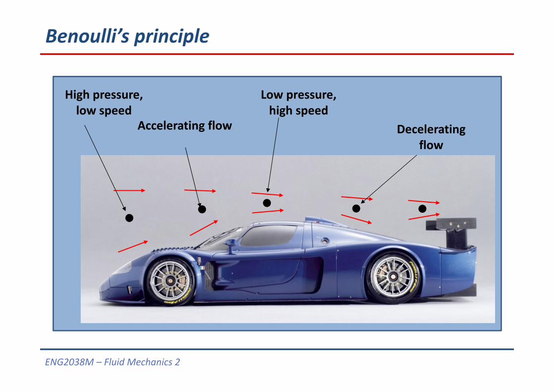
Benoulli’s principle

Accelerating flow Decelerating flow

Low pressure,high speed

High pressure,low speed


Bernoulli's theorem – Fluids 1 lab revision

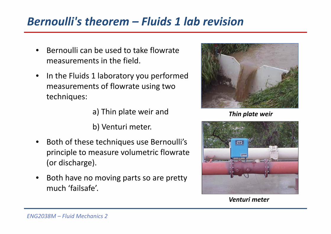
• Bernoulli can be used to take flowrate measurements in the field.

• In the Fluids 1 laboratory you performed measurements of flowrate using two techniques:

a) Thin plate weir and

b) Venturi meter.

• Both of these techniques use Bernoulli’s principle to measure volumetric flowrate (or discharge).

• Both have no moving parts so are pretty much ‘failsafe’.

Thin plate weir

Venturi meter


Bernoulli's theorem – Venturi meter

Venturi meter

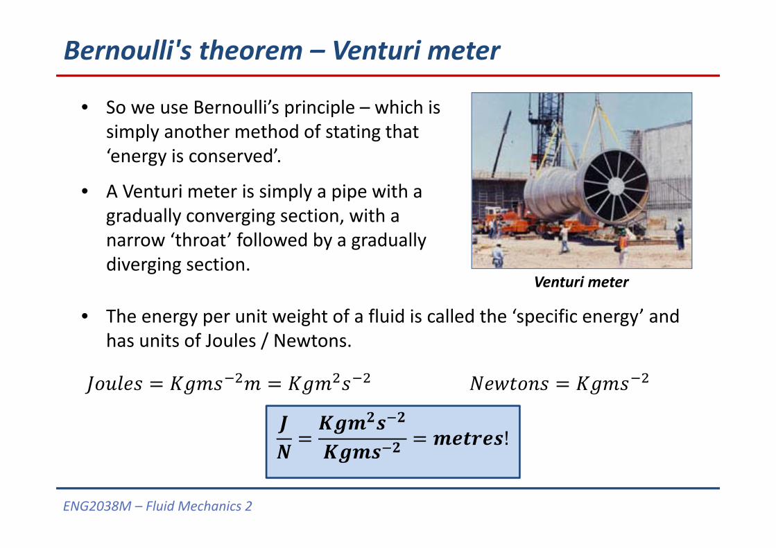
• So we use Bernoulli’s principle – which is simply another method of stating that ‘energy is conserved’.

• A Venturi meter is simply a pipe with a gradually converging section, with a narrow ‘throat’ followed by a gradually diverging section.

• The energy per unit weight of a fluid is called the ‘specific energy’ and has units of Joules / Newtons.

!



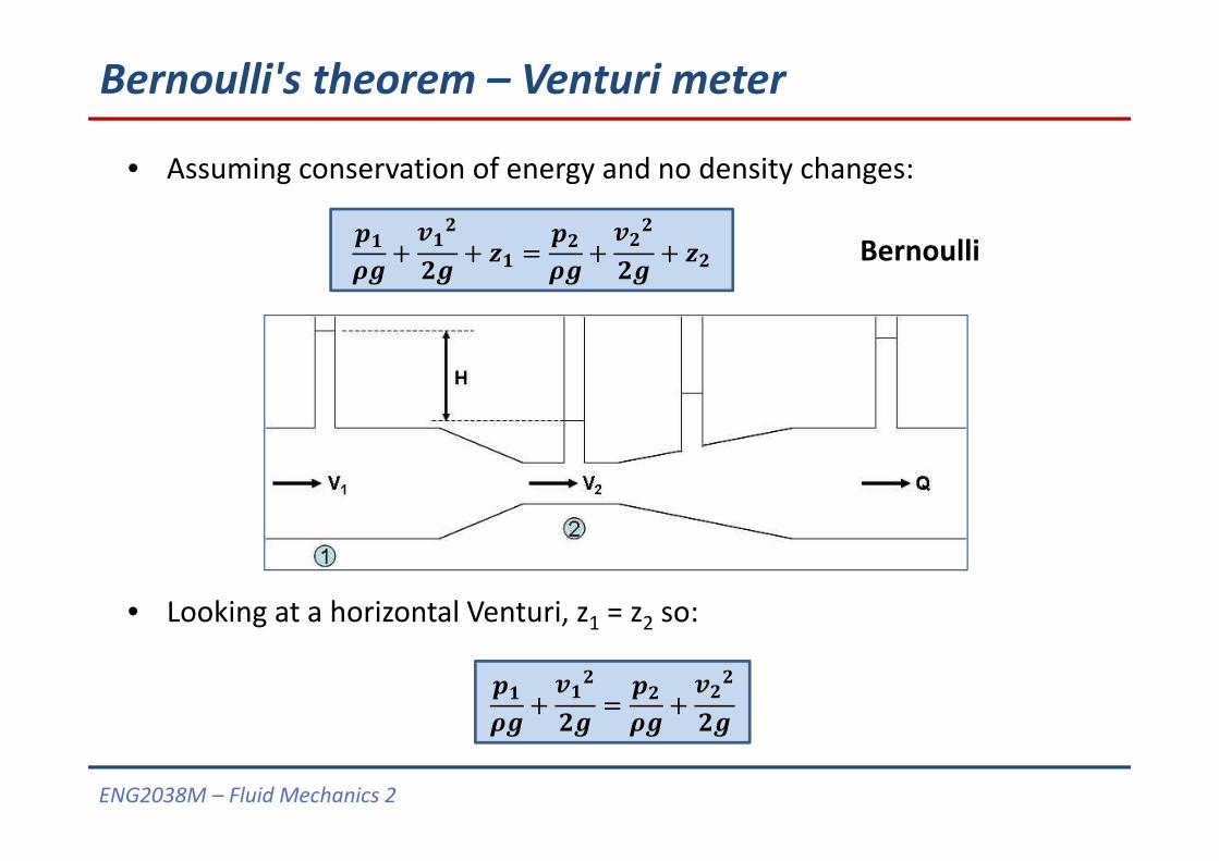
• Assuming conservation of energy and no density changes:

Bernoulli

• Looking at a horizontal Venturi, z1 = z2 so:



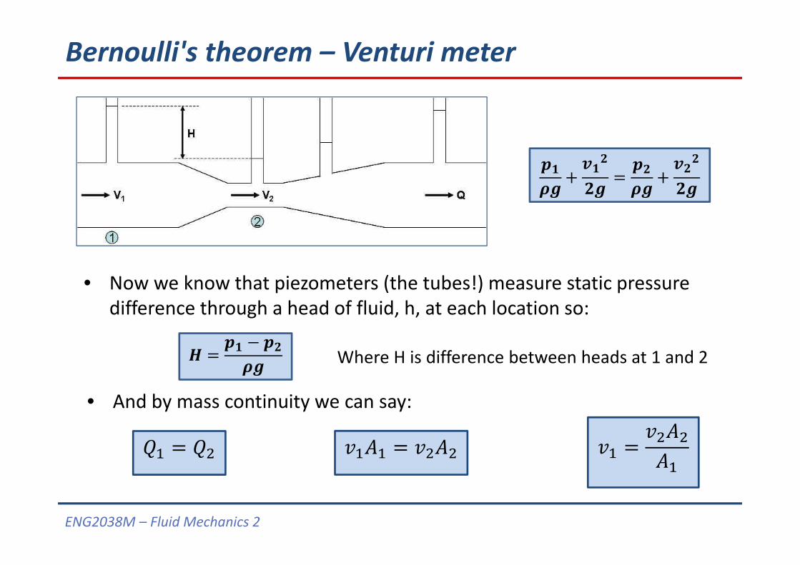
• Now we know that piezometers (the tubes!) measure static pressure difference through a head of fluid, h, at each location so:

Where H is difference between heads at 1 and 2

• And by mass continuity we can say:



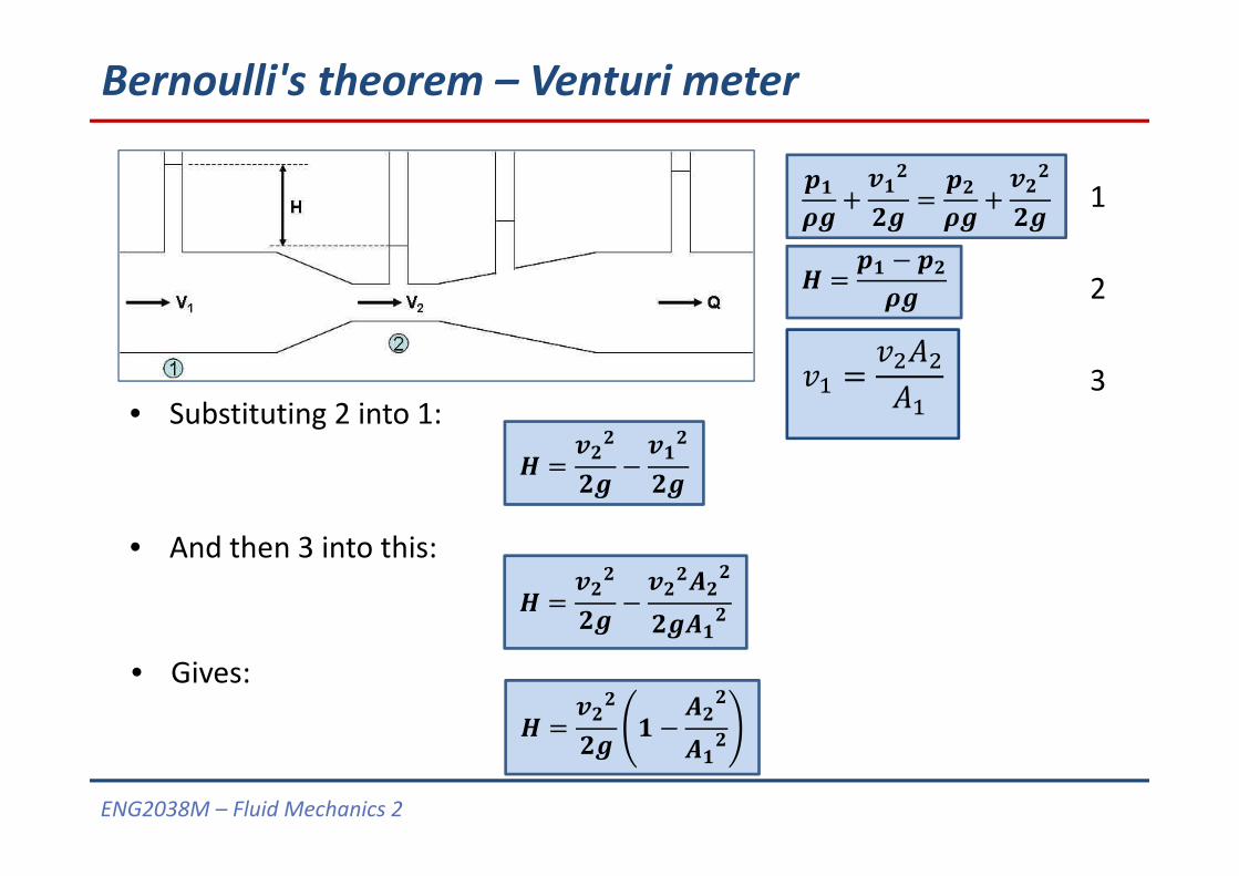
1

2

3• Substituting 2 into 1:

• And then 3 into this:

• Gives:



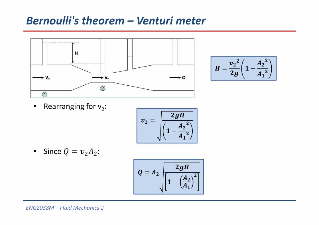
• Rearranging for v2:

• Since :



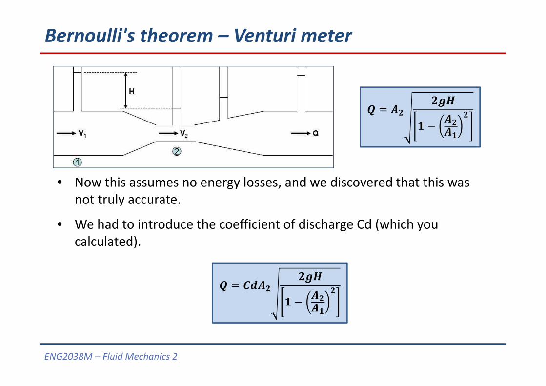
• Now this assumes no energy losses, and we discovered that this was not truly accurate.

• We had to introduce the coefficient of discharge Cd (which you calculated).



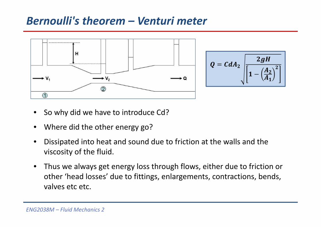
• So why did we have to introduce Cd?

• Where did the other energy go?

• Dissipated into heat and sound due to friction at the walls and the viscosity of the fluid.

• Thus we always get energy loss through flows, either due to friction or other ‘head losses’ due to fittings, enlargements, contractions, bends, valves etc etc.


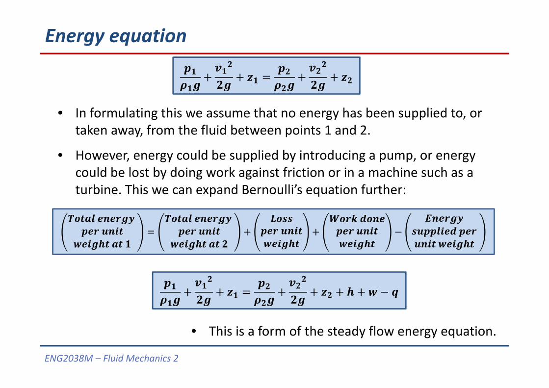
• In formulating this we assume that no energy has been supplied to, or taken away, from the fluid between points 1 and 2.

• However, energy could be supplied by introducing a pump, or energy could be lost by doing work against friction or in a machine such as a turbine. This we can expand Bernoulli’s equation further:

Energy equation

• This is a form of the steady flow energy equation.


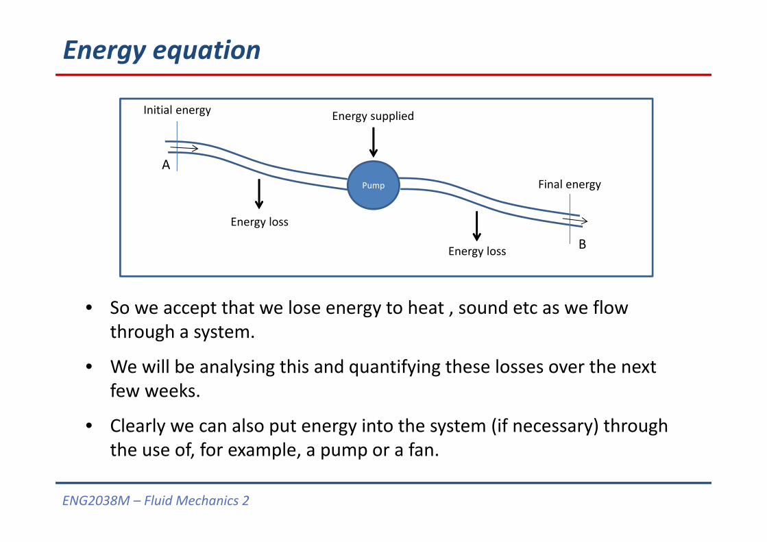
Pump

A

B

Initial energy Energy supplied

Energy loss

Energy loss

Final energy

Energy equation

• So we accept that we lose energy to heat , sound etc as we flow through a system.

• We will be analysing this and quantifying these losses over the next few weeks.

• Clearly we can also put energy into the system (if necessary) through the use of, for example, a pump or a fan.


Energy equation example


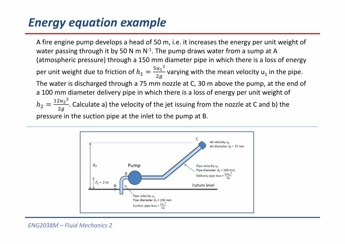
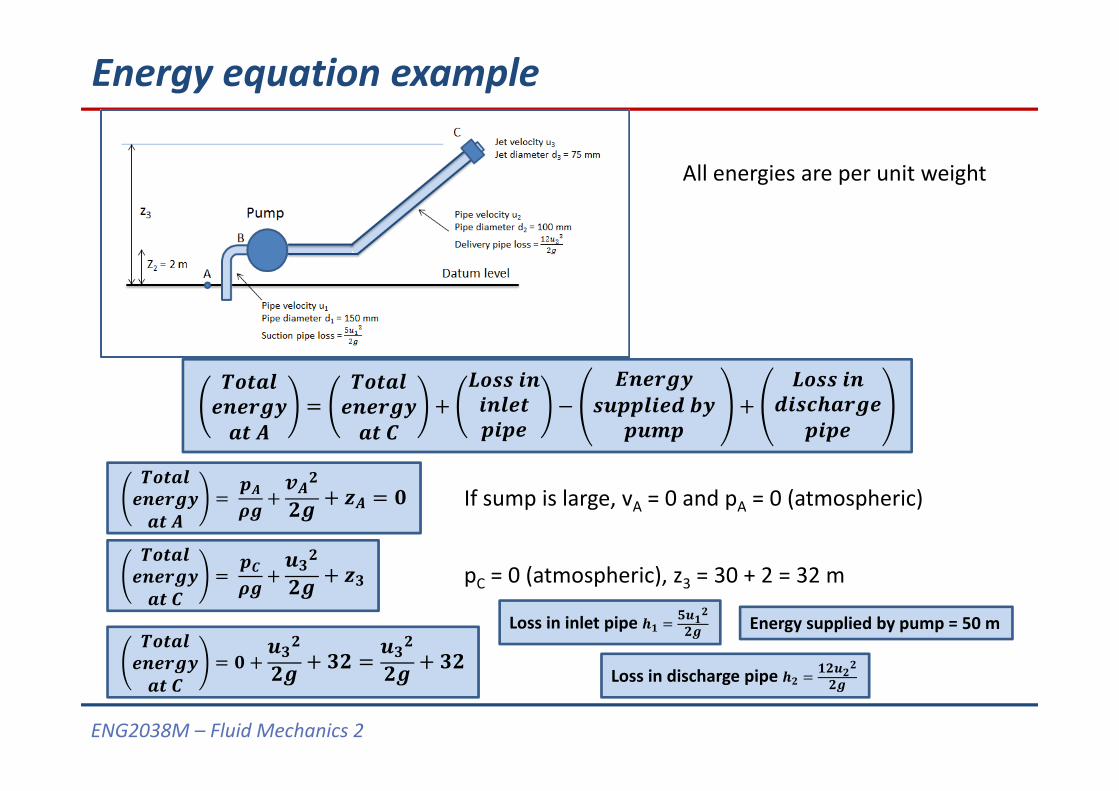
A fire engine pump develops a head of 50 m, i.e. it increases the energy per unit weight of water passing through it by 50 N m N‐1. The pump draws water from a sump at A (atmospheric pressure) through a 150 mm diameter pipe in which there is a loss of energy

per unit weight due to friction of varying with the mean velocity u1 in the pipe.

The water is discharged through a 75 mm nozzle at C, 30 m above the pump, at the end of a 100 mm diameter delivery pipe in which there is a loss of energy per unit weight of

. Calculate a) the velocity of the jet issuing from the nozzle at C and b) the

pressure in the suction pipe at the inlet to the pump at B.




All energies are per unit weight

If sump is large, vA = 0 and pA = 0 (atmospheric)

pC = 0 (atmospheric), z3 = 30 + 2 = 32 m

Loss in inlet pipe

Loss in discharge pipe

Energy supplied by pump = 50 m



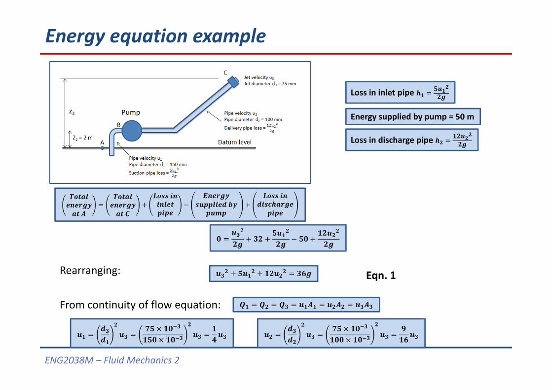
Loss in inlet pipe

Loss in discharge pipe

Energy supplied by pump = 50 m

Rearranging:

From continuity of flow equation:

Eqn. 1



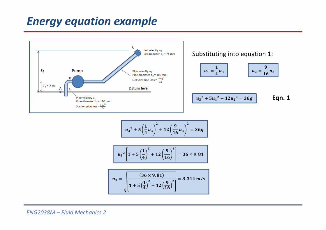
Eqn. 1

Substituting into equation 1:

.

.. /



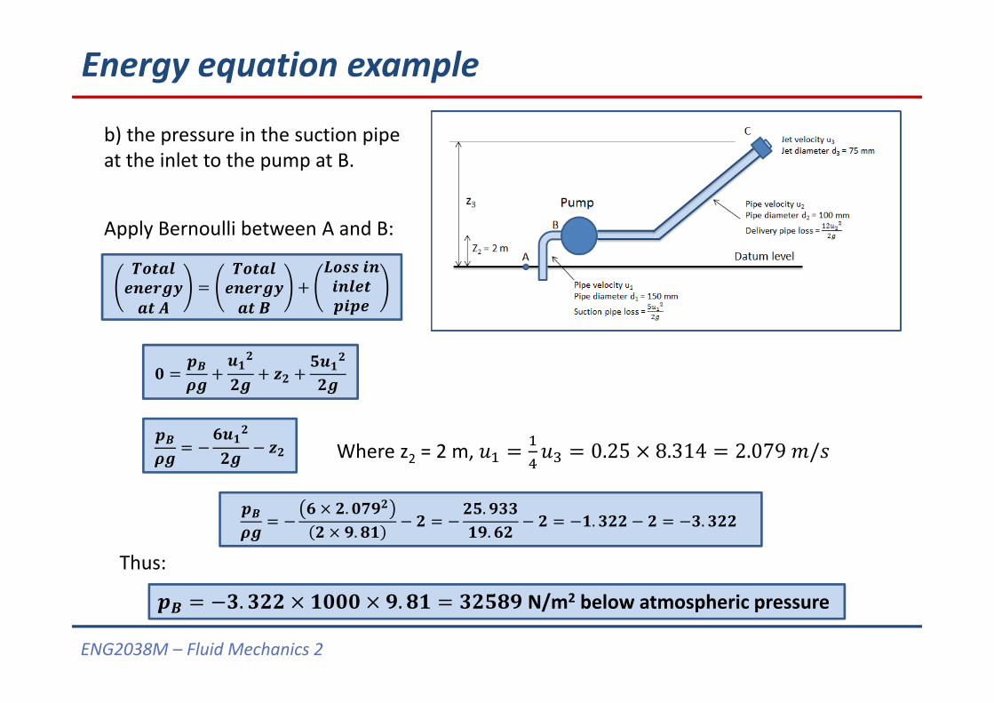
b) the pressure in the suction pipe at the inlet to the pump at B.

Apply Bernoulli between A and B:

Where z2 = 2 m, 0.25 8.314 2.079 /

..

.. . .

. . N/m2 below atmospheric pressure

Thus:

Documents

Lecture 3 The energy equation - skeddanblog · PDF fileENG2038M – Fluid Mechanics 2 Lecture 2 recap Flow Classifications • Conditions in a body of fluid can vary from point to