Lecture 3 Script

Graphs

Slide 1

● To understand graph neural networks, we need to introduce graphs, graph signals, and graph convolutional filters. Let us begin by discussing graphs. This is mostly about the introduction of notation.

Slide 2

● A graph G is a triplet made up of a set of vertices V, a set of edges E, and a set of weights W.

● Vertices, or nodes, are simply a set of n labels, where n represents the total number of nodes in the graph. Typically, labels are the natural numbers from one through n,

● Like in this figure where nodes are labeled 1 through 8

● Edges are ordered pairs of labels of the form i comma j. Where, we emphasize, the ordering is important. In graph signal processing, we interpret the presence of the edge ij in the edge set as a statement that node i can be influenced by node j.

● We denote this influences with pointed arrows. For instance, node 2 can influence node 1 and node 1 has influence over node 3.

● Weights W_ij are numbers that are associated to edges. The weights are interpreted as a representation of the strength of the influence that node j can have on node i. The larger the weight, the larger the influence.

● In the diagram, this is represented with numbers associated to each edge. If w_12 is larger than w_31, it means that the influence 2 has on 1 is larger than the influence 1 has on 3. Only edges have weights associated. There are no weights w_ij if the pair (i,j) is not present in the edge set.

Slide 3

● Let me repeat that the edge (i,j) is graphically represented by an arrow that points from node j into node i. And that this arrow stands in for the fact that node j can have some influence on node i.

● I am repeating this because it is the opposite convention that is common in graph theory. This convention simplifies notation when we define graph shift operators.

● Graphs are classified as directed or symmetric depending on the symmetry of the edge and weight sets. In a directed graph, the edge (i,j) is different from the edge (j,i). It is also possible to have (i,j) be part of the edge set, whereas (j,i) is not part of the edge set.

● For instance, in the figure below there are arrows pointing from node 2 into 4 and from node 6 into 4, but there are no arrows pointing from 4 into either 2 or 6.

● If both edges are part of the edge set, it is still possible to have a difference in the weights. That is, if (i,j) and (j,i) are both in the edge set, we can have W_ij and W_ji be different. In this example graph, we have arrows connecting 3 to 5 in both directions and we also have arrows connecting 5 to 7 in both directions. If the graph is directed, the weight that connects 3 to 5 can be different from the weight that connects 5 to 3. The same holds true for the weights that connect 5 and 7. They can be different as well.

Slide 4

● When there is no directionality on edges or weights the graph is said to be symmetric. For this to happen the edge and weight sets must be symmetric to index transpositions.

● More precisely, edges must come in pairs. Whenever we have (i,j) being part of the edge set, we must have that (j,i) is also part of the edge set.

● In this representative graph, having an arrow pointing from 3 to 5

● Implies that we must have the opposite arrow pointing from 5 into 3.

● In addition to edges being symmetric, weights have to be symmetric as well. We must have that W_ij and W_ji are the same.

● In this particular graph, the weight W_53.

● Must be equal to the weight W_35.

● This is something that we can signify with a double pointed arrow and a single weight.

● If all edges are connected in both directions with all weights being symmetric, as is shown here, the graph is symmetric.

Slide 5

● Weights are not always necessary. When a graph doesn’t have weights, we say that it is unweighted.

● Sometimes it is convenient to equivalently interpret an unweighted graph as one in which the weights are units, that is, one in which W_ij is 1 for all edges in the edge set.

● Unweighted graphs can also be directed, as the one we are showing below.

● Or undirected, as the one we are showing now.

Slide 6

● Graphs can be directed or symmetric. and they can be weighted or unweighted. These are separate classes. The four combination are possible.

● Most of the graphs that we encounter in practice are symmetric and weighted. This will be the case in the problems we will study in the labs.

Graph Shift Operators

Slide 7

● It is standard to represent graphs with adjacency and Laplacian matrices. In the context of graph signal processing, these matrix representations of a graph are called graph shift operators.

Slide 8

● The adjacency matrix of a graph G, is the sparse matrix A whose non-zero entries record the weights of the graph.

● Specifically, the i comma j entry of A is non-zero if and only if (i,j) is an edge of the graph. In which case, the value of the entry is the weight W_ij.

● In the example we have a symmetric graph. The weights on the edges that connect 1 and 2 are recorded in the corresponding entries of the adjacency matrix. They are row-one-column-two as well as row-two-column-one.

● Likewise, the weights in the edges that connect 1 and 3 are recorded in the entries of the adjacency matrix that correspond to row-one-column-three as well as to row-three-column-one.

● The remaining non-zero weights are recorded in the corresponding row and column of the adjacency matrix A.

● And the rest of the matrix is filled with zeros.

● When the graph is symmetric, the adjacency matrix is symmetric as well.

● That is, the adjacency matrix and its transpose coincide.

● As is the case of the adjacency matrix we have covered in this example.

Slide 9

● For the particular case of unweighted graphs, we recall that weights can be interpreted as units. Therefore, the i comma j entry of the adjacency matrix A, is 1 whenever the corresponding edge (i,j) belongs to the edge set. We show here an unweighted version of the graph we have just seen. The node set and the edge set are the same, but the weights are 1 in all edges. The adjacency matrix has the same sparsity pattern as before, except that now all non-zero entries are 1.

● For instance, the edges connecting 1 and 2 generate entries in A, in row one column two and row two column one. These entries are units

● The edges connecting 1 and 3 generate entries in A corresponding to row one column three and row three column one. These entries are units as well

● The remaining edges generate the remaining non-zero entries of the adjacency matrix A.

Slide 10

● The edge set of a graph can be described in terms of neighborhoods to emphasize the locality of influence. The neighborhood of node i is the set of nodes that are sources of arrows that point into node i. Or more formally, the set of nodes j for which (i,j) is part of the edge set.

● In the example, the neighborhood of node 1 is made up of nodes 2 and 3.

● We also define the degree of a node. The degree of node i is denoted as d sub i, and is given by the sum of the weights in all of its incident edges. Namely, the sum of the weights in all of the edges that connect i from some of its neighbors.

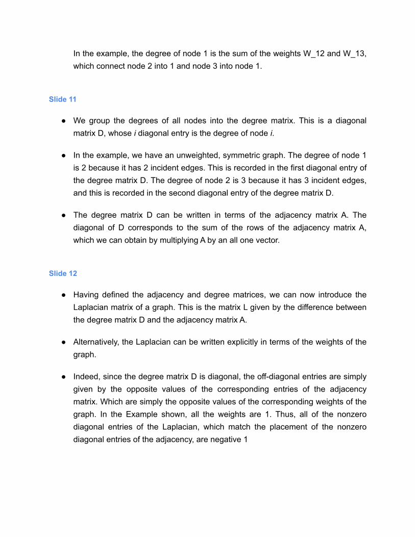
In the example, the degree of node 1 is the sum of the weights W_12 and W_13, which connect node 2 into 1 and node 3 into node 1.

Slide 11

● We group the degrees of all nodes into the degree matrix. This is a diagonal matrix D, whose i diagonal entry is the degree of node i.

● In the example, we have an unweighted, symmetric graph. The degree of node 1 is 2 because it has 2 incident edges. This is recorded in the first diagonal entry of the degree matrix D. The degree of node 2 is 3 because it has 3 incident edges, and this is recorded in the second diagonal entry of the degree matrix D.

● The degree matrix D can be written in terms of the adjacency matrix A. The diagonal of D corresponds to the sum of the rows of the adjacency matrix A, which we can obtain by multiplying A by an all one vector.

Slide 12

● Having defined the adjacency and degree matrices, we can now introduce the Laplacian matrix of a graph. This is the matrix L given by the difference between the degree matrix D and the adjacency matrix A.

● Alternatively, the Laplacian can be written explicitly in terms of the weights of the graph.

● Indeed, since the degree matrix D is diagonal, the off-diagonal entries are simply given by the opposite values of the corresponding entries of the adjacency matrix. Which are simply the opposite values of the corresponding weights of the graph. In the Example shown, all the weights are 1. Thus, all of the nonzero diagonal entries of the Laplacian, which match the placement of the nonzero diagonal entries of the adjacency, are negative 1

● As for the diagonal entries, assuming the graph has no self loops, the diagonal entries of the adjacency matrix A are null. Therefore the diagonal entries of the Laplacian are simply the diagonal entries of the degree matrix D.

Slide 13

● Normalized versions of the adjacency and Laplacian matrices are also utilized as matrix representations of graphs.

● The normalized adjacency is defined by pre and post multiplication by the inverse square root of the degree matrix. The resulting entries divide graph weights by the square root of the degrees of the incident nodes. The interpretation is that weights are re-expressed relative to the degrees of their incident nodes.

● The normalization is such that if the graph is symmetric, the normalized adjacency matrix is symmetric. The normalization has been chosen to have this property. This is why we pre- and post- multiply by the degree matrix.

Slide 14

● The normalized Laplacian is defined in the same manner by pre and post multiplication by the inverse square root of the degree matrix D. As in the case of the adjacency, weights end up expressed relative to the degrees of their incident nodes.

● Indeed, given the definitions of the normalized operators and the definition of the Laplacian as the subtraction of the degree matrix from the adjacency matrix, it follows that the normalized Laplacian can be written as the difference between the identity matrix and the normalized adjacency.

● Thus, off-diagonal entries are the opposite of the off-diagonal entries of the normalized adjacency. More importantly, since the diagonal components are an identity matrix, the normalized adjacency and the normalized Laplacian are essentially the same linear transformation. There is no substantial difference between A bar times x and L bar times x.

● The value of normalized operators lies in that they are more homogeneous representations when we consider heterogenous graphs where different nodes differ substantially in their respective degrees. The sum of the values contained in each row and column of the normalized operators are more similar across different indexes. When these differences are undesirable, normalized operators are useful.

Slide 15

● The Graph Shift Operator S is a stand in for any of the matrix representations of the graph.

● We can make it equal to the adjacency matrix,

● Equal to the Laplacian matrix,

● Or the normalized adjacency,

● Or the normalized Laplacian.

● And, of course, if the graph is symmetric, the shift operator S is symmetric as well.

● The reason for defining the shift operator is that a specific choice matters in practice, but most results and analysis hold for any choice of tests. A different version of this statement is that we don’t have to worry about the choice of shift operator during our mostly analytical lectures. Although you will have to worry about that in your practical implementations during labs.We will therefore use a generic shift operator S, in our definitions of graph convolutions and graph neural networks.

Graph Signals

Slide 16

● Graph signals are the objects we process with graph filters and graph neural networks

Slide 17

● Begin with a graph G having n nodes and shift operator S.

● A graph signal is a vector, which also has n components and in which we associate component x_i to the i-th node of the graph. In the diagram, we show a graph with eight nodes supporting a graph signal with eight components. Different components of the signal are associated to different nodes of the graph,. Something that we represent by scaling the size of the nodes.

● Although a graph signal is just a vector, the shift operator is considered intrinsic to the signal. When we want to emphasize this fact, we write the signal as a pair made up of the shift operator and the signal itself.

● The graph is an expectation of proximity or similarity between the components of the signal x and the objective of graph signal processing is to leverage this prior information in the processing of the signal.

Slide 18

● Multiplication of a graph signal by a shift operator implements a diffusion of the signal over the graph.

● More formally, define a diffused signal y as the product of the graph shift operator with a given graph signal x.

● Because of the sparsity pattern of S, the i-th component of the diffused signal, which we denote by y_i, is affected only by the components that we denote by x_j for j in n of i. These are the values of the input signal x that are supported on adjacent nodes j that belong to the neighborhood of i. In a normal matrix multiplication we would sum over all j indexes. But only the weights in the neighborhood of i are nonzero in the product S times x.

● In the illustration, we have an input graph signal with components x_i and we highlight the input value at node 2. The result of the diffusion operation at this node is affected only by the values of the input signal x_j at the neighboring nodes that we highlight in green. The diffusion value y_2 is affected by the input value x_4. But it is not affected by x_8.

● Notice that the converse of this influence statement dictates that the value of the input x_i associated with node i affects the values of the diffused signal y_j only for the indexes j that correspond to neighboring nodes. In the example here, the value x_2 of the input signal at node 2 affects the values of the diffused signal y_j only at those nodes j that are neighbors of i which we highlight in green. The input value x_2 affects the output value y_4. But it does not affect y_8

● Further observe that stronger weights contribute more to the output of the diffusion. Thus, the locality of the diffusion manifests also on the strength of the influence that node j has on node i. This is important when graphs are not that sparse but have dominant weights.

● We summarize these observations by saying that diffusion is a local operation whereby signal components are mixed with signal components of neighboring nodes. This is a property that is natural to leverage in the processing of the signal x. And it also plays an important role in the use of diffusions in distributed systems.

Slide 19

● The diffusion operator can be composed with itself to produce the diffusion sequence.

● We formally define this sequence through recursive multiplication by the shift operator S. Element 0 is the signal itself. And subsequent components are such that k plus first element of the diffusion sequence is the product of S and the k-th element of the diffusion sequence.

● To be more clear, the zeroth entry of the diffusion sequence is the graph signal itself.

● Element one is the diffusion of element 0. This is the diffused signal Sx we have just discussed.

● Element two of the diffusion sequence is the diffusion of element 1. This is the diffusion of the diffused signal.

● Element three of the diffusion sequence is the diffusion of element 2. The diffusion of the diffusion, of the diffusion. If you want to keep track.

● Alternatively, we can unroll the recursion and simply write the kth entry of the diffusion sequence as the k-th power of the graph shift operator S applied to the input graph signal x.

● Entry zero of the diffusion sequence is the multiplication of the shift operator raised to the power of 0 with the graph signal. This is the graph signal itself.

● Entry one of the diffusion sequence is the product of S raised to the power of 1 with x. This is the diffused signal.

● Entry two is obtained by premultiplying the signal x with the shift operator S raised to the power of 2.

● And entry three two is obtained by premultiplying the signal x with the shift operator S raised to the power of 3.

Slide 20

● Some observations are in order.

● The diffusion sequence embeds the trade off between local and global information. As we can see from the their definitions, and perhaps more clearly from the figures, the k-th element of the diffusion sequence diffuses information to and from k-hop neighborhoods. Thus, for low values of k the entries of the diffusion sequence represent local information only. Whereas, for large values of k, the entries of the diffusion sequence represent global information.

● This trade off between locality and globality is a characteristic of convolutions. We know already, and we are going to see it again in the next video, that the diffusion sequence is used in the definition of graph filters. This is one reason why. Not the only. But certainly one.

● There are two equivalent versions of the diffusion sequence. One recursive, and one using powers of the shift operator S.

● Be warned to always use the recursive version in implementations. This warning bears repetition. Always. I repeat. Always, use the recursive definition of the diffusion sequence. There are dramatic differences in computational cost. Incidentally, when we consider distributed systems, this is the only version that can be utilized.

● The power version is the one we will use for analyses.

Graph Convolutional Filters

Slide 21

● Graph convolutional filters are the tool of choice for the linear processing of graph signals.

Slide 22

● Given a graph shift operator S and a possibly infinite set of coefficients h_k, a graph filter is defined as a polynomial on the shift operator with coefficients h_k. Or a series, if you want to be precise when the number of coefficients is infinite. The resulting graph filter is a matrix that we denote by H of S.

● Applying the filter to a graph signal x entails multiplication of the signal x with a graph filter H of S to produce the output signal y.

● We group the coefficients h_k in a sequence we call h. We then say that y is the graph convolution of the filter h with the graph signal x. We use the familiar convolution notation annotated with a sub index S to indicate the use of the shift operator in its definition.

Slide 23

● Perspicacious listeners may have noticed the appearance of the diffusion sequence in the definition of graph convolutional filters. They will therefore not be surprised to see us highlighting the fact that graph convolutions aggregate information growing from local neighborhoods into global neighborhoods. Which as we have said several times already, is an important property of convolutions.

● To revisit this important point, consider a signal x, supported on a graph with shift operator S. Along with a filter h with coefficients h_k. The filer contains K taps. From 0 to K-1.

● For this given signal, graph and filter, we undertake the computation of the output of the convolution of h with x on the graph S.

● We begin with an illustration of the graph on which the signal components are supported on individual nodes.

● To compute the output of the graph convolution we begin with the graph signal x itself, which we scale with coefficient h zero. We highlight the signal value at node 4.

● To the signal x we add the diffusion S times x, which we scale with coefficient h one. This results in the convolution output at node 4 being affected by all of its one-hop neighbors.

● To the resulting sum we add the product of S raised to the power of two with x scaled by coefficient h_2. This represents a diffusion of the diffused signal. Adding this term to the convolution results in the value at node 4 being affected by all of its two-hop neighbors.

● We then add the product of S raised to the power of three with the signal x modulated by coefficient h_3. This is the third component of the diffusion sequence which we know aggregates information from 3-hop neighbors.

● To complete the graph convolution we keep adding components of the diffusion sequence scaled by their respective filter coefficients until we reach the order of the filter. The last entry, is the capital K minus 1 element of the diffusion sequence scaled by coefficient capital K-1.

Slide 24

● A separate important property of graph convolutions is that the same filter can be executed in multiple different graphs. This is because the graph filter and the shift operator are separate from each other in the definition of the graph filter. They have to be designed jointly, of course, but the coefficients h_k do not depend on the shift S afterwards.

● We say that we can transfer the filter across graphs.

● To illustrate this point consider a signal supported on a graph. The same one we consider a minute ago.

● And a different signal supported on a different graph.

● To write the convolutions output we proceed as before.

● We start with the signal x scaled by coefficient h_0. This is the same operation on both graphs.

● We then add the diffusion S times x modulated by coefficient h_1. The resulting operations are different in different graphs. Because the graph neighborhoods are different. This is highlighted for node 4 in both graphs.

● The same is true of element 2. The same notation, namely, the shift S raised to the power of two multiplying x and the result scaled by h_2, represents different operations when instantiated in different graphs.

● And the same holds for element 3 of the diffusion sequence. Same abstract operation. Different instantiated results.

● Upon completing the execution of the filter, the convolutions could be quite different. Because the graphs are different. But it is nevertheless possible to move the filter from one graph to another. This is true no matter how different the graphs are. They can have different neighbors. Different weights. Different numbers of nodes, even.

● I don’t want to make too much of a big deal of this. I am just saying that the output of a graph convolution depends on the filter coefficients and the shift operator S and that these two can be chosen separately. But the ability to transfer a filter across graphs will prove to be very important to us. In both theory and practice. It is all but impossible to encounter the exact same graph twice. Our theory and practice have to account for that.

Slide 25

● A graph convolution is a weighted linear combination of the elements of the diffusion sequence. Which, we recall, we can compute with matrix powers or with recursive application of the shift operator.

● Using the recursive definition of the diffusion sequence we end up with a shift register structure. Which is familiar to those of you that have studied implementation of graph filters. Familiar or not, the shift register is just a visualization of the recursive computation of the diffusion sequence. It is based on interpreting convolutions as a combination of scaling, shifting, and summing.

● Start with the signal x, which we write as S to the power of 0 time x. This is the shifting.

● We scale by h_0.

● We sum towards the output.

● We now multiply this signal by the shift operator S. This is the shifting.

● It produces the signal S to the power of 1 times s. Element 1 of the diffusion sequence.

● We scale by h_1

● We sum towards the output. We accumulate, if you wish.

● We multiply by S a second time. This is the shifting.

● It produces entry 2 of the diffusion sequence. The signal S to the power of 2 times x.

● We scale by h_2.

● We sum towards the output

● We multiply by S once more. Another shift.

● It produces entry 3 of the diffusion sequence. S to the power of 3 times x.

● Scale by h_3.

● And sum towards the output.

● Since this is a filter with 4 taps, the accumulated sum is the output of the convolutional graph filter. This shift register structure is the one we use in the implementation of graph filters. We shift. We scale. We sum.

Time Convolutions as a Particular cases of Graph Convolutions

Slide 26

● We have already seen that time convolutions are particular cases of graph convolutions. This is how we motivated their introduction. But now we have seen

graph convolutions in closer detail, we can investigate their connections further. We will work with the shift register representation of graph filters.

Slide 27

● Time convolutional filters process signals in time by leveraging the time shift operator.

● In the figure, we show a signal in which we highlight some components.

● The time shift operator advances the signal components in time so that the component that used to be located at the time zero is now located at time one, and the component that used to be located at time one is now located at time two.

● Time shifts can be composed. In the same way in which we composed graph shift operators. A second shift moves the signal component that used to be at the time zero into time two.

● And a third shift moves the signal component that used to be located at time zero into time three. These time shifted signals can be added to produce the output of a time convolutional filter.

● This convolution is represented by the familiar shift register structure.

● We begin with the original unshifted signal x, which we scale by coefficient h zero.

● We continue by adding a shifted copy of the original input signal x, scaled by coefficient h one.

● To the resulting sum, we add the twice shifted version of the input signal, scaled by coefficient h two.

● And we further add a thrice shifted version of the input scaled by h_3,

● We keep shifting summing and scaling until the order of the filter. To have the time convolution of filter h with signal x written as a linear combination of time shifted versions of the input signal x. The coefficients of the linear combination are the filter taps h_k

Slide 28

● Time signals can be equivalently represented as graph signals supported on a line graph and time shifting as multiplication by the adjacency matrix of this graph.

● To look at the details of how this is done, let’s look again at our time signal x.

● We can reinterpret this time signal as a graph signal if we associate instants in time with nodes of a graph and add directed edges connecting node n to node n + 1. These edges signify the proximity and causality of time. Node n + 1 can be influenced by node n. Node 0 influences Node 1. Node 1 influences Node 2; which influences 3, and so on.

● What we have done is to rewrite our time signal as a pair S comma x, where S is the adjacency matrix of the line graph. This is overkill. We already know how to process time signals. But instructive. And also true. A time signal is a pair made up of the adjacency of the line graph and the signal itself. However implicit, we often leave the presence of the graph.

● Using this alternative and equivalent representation of time signals, we can rewrite the time shift operation as a multiplication with the adjacency matrix of the line.

● As we show in this equation, all of the entries of this adjacency matrix are zero. Except for those in the first sub diagonal which are one because the graph is unweighted.

● When we premultiply the signal x with the adjacency matrix S.

● The result is a reallocation of the components of x. They move one place down in their position. Save for the first and last entry, the output of the operation has the same components. But the entry x_i associated to index i in vector x, is now associated with index i + 1 in the output vector.

● If we look at the graph representation of our time signal, the components are shifted to the next node of the graph. They follow the arrows, to speak informally. Ot they diffuse through the edges, to speak more accurately.

● These multiplications can be composed. Begin by considering the product of S raised to the power of 2 with x.

● This is equivalent to multiplying by S a second time. We therefore have to compute the product of S with the shifted vector S times x.

● But we already know that the effect of this product is to shift signal components. To move the place of components down relative to their position in the input vector. But this time we are shifting an already shifted signal. We therefore end up with an output in which components are shifted two places. Except for the borders of the vector, the entry x_i associated to index i in vector x, is now associated with index i + 2.

● If we look at the graph representation of the time signal, the components are shifted to the next node of the graph. The diffuse through the edges a second time.

● We now move on to S to the power of 3 times x.

● This can be recursively computed as the product of S with S squared times x.

● And we know that the effect is to produce a shift of the indexes one place down. Which, since we are applying the shift to a twice-shifted signal, results in a thrice-shifted signal.

● In the graph representation of the time signal, the components diffuse one node up through the edges of the graph.

● The important point to observe is that the application of subsequent powers of the adjacency S to the time signal x is equivalent to the subsequent application of time shifts.

● We can therefore rewrite time convolutional filters as multiplications with polynomials of the adjacency matrix of the line graph.

Slide 29

● Indeed, let us return to our definition of the convolution as a linear combination of shifted versions of the input.

● This is a structure that a few minutes ago we represented with this shift register.

● But we now know that all of the time shifts that appear in the register are equivalent to multiplications with the adjacency matrix S of the line graph.

● That is, the time signal can be written as a graph signal supported on a line graph and subsequent shifts can be rewritten as multiplication by its adjacency S. Therefore, in all of the places in which a shift operator appears in the register.

● We can equivalently write a multiplication with a power of the adjacency matrix S.

● This block diagram and the mathematical expression its represents is nothing but the expression we had before for a graph convolutional filter when we particularize it to the adjacency matrix of a line. Thus, as we had said at the beginning of this video, the time convolution operation is a graph convolution applied to this specific graph.

Slide 30

● We have revisited time convolutions to show that they are particular cases of graph convolutions. While we are here, we can take some time to see how graph convolutions are obtained as generalizations of time convolutions.

● To obtain this generalization we just have to let the graph shift operator be arbitrary. This shift register represents a convolution in time only because the operator S is the adjacency of a line graph.

● But if S denotes the adjacency of an arbitrary graph, this is an arbitrary graph convolution.

● When we apply the shift operator, the signal diffuses in a different manner. Signal components are now following a different set of arrows.

● But we can still compose diffusion a second

● Or a third time. By the expedient modification of changing the graph. The shift register is now a representation of a graph convolution on a different graph. The notion of diffusion is different, but the structure of the shift register that defines the convolution stays the same.

Graph Fourier Transform

Slide 31

● Fourier transforms are an important tools for analyzing information processing systems. In the case of graphs, the tool takes the form of the graph Fourier transform.

Slide 32

● We start with some preliminary assumptions. We will work with symmetric graphs having symmetric shift operators with S equal to S Hermitian.

● For shift operator S we use v_i to denote its eigenvectors and lambda_i to denote its eigenvalues. If you need a reminder, eigenvectors are those that do not

change direction when multiplied by S. They are just scaled. The eigenvalue is the scaling factor.

● For a symmetric S, eigenvalues are real and they can be therefore be ordered. We assume here that increasing index represents increasing eigenvalues.

● We group the eigenvectors as columns of the eigenvector matrix V. We group eigenvalues as diagonal entries of the diagonal eigenvalue matrix Lambda.

● With these definitions we can write the eigenvector decomposition of the graph shift operator as the product V times Lambda times V Hermitian.

● In this expression we have that V Hermitian times V is the identity. This is because the graph is symmetric.

Slide 33

● We use the eigenvector decomposition of the shift operator to define the graph Fourier transform.

● For a shift operator with eigenvector matrix V.

● The graph Fourier transform of a signal x supported on S is the signal tilde x given by the product of V Hermitian with x.

● This definition says that the GFT of signal x is its projection on the eigenvector basis of the shift operator. We will say projection on the eigenspace to save words.

● The GFT tilde x is said to be the graph frequency representation of x. And that tilde x is a representation in the graph frequency domain.

Slide 34

● We can also define an inverse transform.

● For a shift operator with eigenvector matrix V.

● The inverse graph Fourier transform of what is presumably a GFT signal tilde x is the signal x-double-tilde given by the product to V with tilde x. Notice that we use the matrix V here. Not V Hermitian as in the definition of the GFT.

● This inverse transform is a proper inverse of the GFT because the iGFT of the GFT of the signal x is the signal x itself.

● In case you have never seen a proof of this fact, write the definition of the iGFT. If we assume the blue signal tilde x whose inverse we are computing, is the GFT of signal x.

● We can use the definition of the GFT to write it as V Hermitian time x. In this expression we have the product V times V Hermitian.

● We know that this is an identity matrix.

● And multiplying by an identity matrix is moot.

Graph Frequency Response of Graph Filters

Slide 35

● We have defined graph convolutional filters and we have seen that they are a valid generalization of time convolutional filters.

● We will see now that graph filters admit a pointwise representation when projected in the graph frequency domain. This is another fundamental property they share with time convolutional filters.

Slide 36

● The GFT can be leveraged to represent graph filters in the graph frequency domain. We introduce this representation as a Theorem.

● Consider then a graph filter h with coefficients h_k. A graph signal x. And a filtered signal y defined as a polynomial on the adjacency matrix modulated with coefficients h_k.

● If we introduce the GFTs tilde x and tilde y of the input and output signal, we can relate the GFTs through multiplication with a polynomial on Lambda modulated by coefficients h_k. That is, the GFT tilde y is the product of the polynomial we highlight in red with the GFT tilde y. The matrix that appears in this polynomial is Lambda. The diagonal matrix that contains the eigenvalues of the graph shift operator.

● It is pertinent to remark that the two polynomials that appear in this theorem are the same but on different variables.

● The polynomial that defines the graph filter is on S.

● And the polynomial that defines the frequency representation is on Lambda. The variables are different. But their coefficients are the same.

Slide 37

● Before we elaborate more on the consequences of this theorem, let’s give a proof.

● Recall that the spectral decomposition of the shift operator says that S equals V times Lambda times V Hermitian. It follows that S to the power of k can be written as V times Lambda to the power of k times V Hermitian.

● Thus, the filter that we write here with its usual definition.

● Can be rewritten by replacing power of S by these factors containing powers of Lambda

● Multiply now on the left by V Hermitian on both sides of the equality. Doing so yields some familiar terms.

● Let’s copy the expression so that we can start identifying them.

● The product V Hermitian times y is nothing but the GFT of the output signal. We write this down into an equality we are building on the right side of the slide.

● The product V Hermitian times x is nothing but the GFT of the input signal. We write that down on the right.

● Among the remaining terms, look at the ones involving V Hermitian and V. These terms cancel out because V Hermitian times V is an identity.

● We are left with the terms in red that we copy to the right side

● This is the result that we wanted to prove.

Slide 38

● We have just proven that in the GFT domain, filters are diagonal. Such a diagonal relationship between the Graph Fourier transforms at the input and output of a graph filter.

● Implies that graph convolutions are pointwise operations in the GFT domain. This is true because all that goes on in a multiplication by a diagonal matrix, is that the i-th component of the input is multiplied by the i-th diagonal entry.

● In our particular case, we have that the i-th component of the GFT of the output .

● Is the product between the i-th component of the GFT of the input.

● And the corresponding diagonal element. Which is associated with the i-th eigenvalue of the graph shift operator.

● This is a very simple observation. In fact, its simplicity is rather the point. But nevertheless one that is insightful. To explore the insights that follow from this observation, we define the graph frequency response of a graph filter.

● Given a graph filter with coefficients h

● The frequency response of the graph filter is defined as a polynomial on a scalar variable lambda modulated by coefficients h_k. This is the same polynomial that defines the filter. And the same one that represents the filter in the frequency domain. But the variable of this polynomial is scalar.

● The definition of the frequency response is such that we can write the i-th component of the output GFT as the product between the i-th component of the input GFT and the graph frequency response evaluated at the corresponding eigenvalue lambda i.

Slide 39

● Some observations are in order.

● As we have already pointed out, we emphasize that the frequency response is the exact same polynomial that defines the graph filter.

● Except that instead of being a polynomial on the shift operator, it is a polynomial on a scalar variable lambda.

● A second observation that follows from this one, is that the frequency response is independent of the graph. This is a very important observation that bears repetition. The graph frequency response does not depend on the specific graph.

● It is completely determined by the filter coefficients.

● In a graph filter, the role of the graph is to determine the eigenvalues on which the response is instantiated. But it doesn't play a role in the values that the graph frequency response itself takes.

Slide 40

● To explain this points better we show an illustration of a graph frequency response. It’s just a single variable analytic function.

● It is completely determined by the filter coefficients. The graph has nothing to do with it.

Slide 41

● What is then the role of the graph?

● Well, when given a specific graph, the response is instantiated on its specific eigenvalues lambda_i.

● And when we are given a different graph, the response is instantiated on a different set of eigenvalues hat lambda_i.

● Thus, first and foremost, the graph determines the eigenvalues of the response that are instantiated when the filter is run on a particular graph. This is a deep observation. It allows us to study the effect of running the same filter on different graphs. This is how we will obtain stability and transferability results.

● It is notable that eigenvectors do not appear here. But we have to remember that eigenvectors are associated to eigenvalues. Their role is to specify the instantiation of a frequency component.

Time Estimates for Recordings ● It takes about 2.4 minutes per page.

● It takes about 3.8 minutes every 2 pages

● A script that covers about 7 minutes takes about 3 pages.