Lecture 3

Review of Linear Algebra

Simple least-squares

9 things you need to remember from Linear Algebra

Number 1

rule for vector and matrix multiplication

u = Mv ui = k=1N Mik vk

P = QR Pij = k=1N Qik Rkj

Sum over nearest neighbor indices

Name of index in sum irrelevant. You can call it anything (as long as you’re consistent)

Number 2

transpostionrows become columns and columns become rows

(AT)ij = Aji

and rule for transposition of products

(AB)T = BT AT

Note reversal of order

Number 3

rule for dot product

ab = aT b = i=1N ai bi

noteaa is sum of squared elements of a

“the length of a”

Number 4

the inverse of a matrix

A-1 A = I

A A-1 = I

(exists only when A is square)

I is the identity matrix

1 0 0

0 1 0

0 0 1

Number 5

solving y=Mx using the inverse

x = M-1y

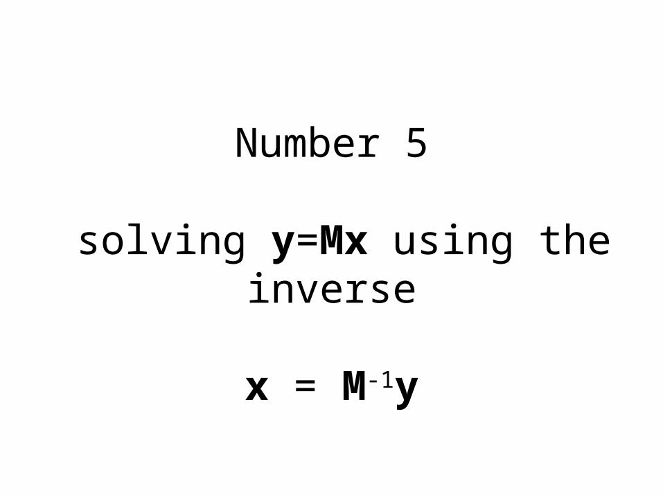
Number 6multiplication by identity matrix

M = IM = MI

in component notation Iij = ij

k=1N ik Mkj = Mij

k=1N ik Mkj = Mij

Just a name …

Cross out sum

Cross out ik

And change k to i in rest of equation

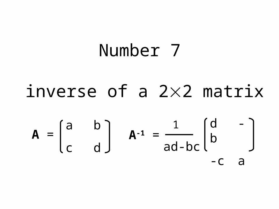
Number 7

inverse of a 22 matrix

a b

c dA =

d -b

-c aA-1 =

1

ad-bc

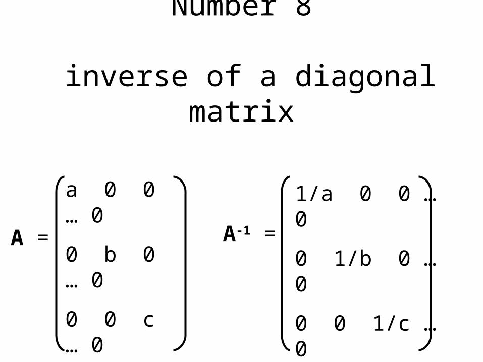
Number 8

inverse of a diagonal matrix

a 0 0 … 0

0 b 0 … 0

0 0 c … 0

...

0 0 0 …z

A = A-1 =

1/a 0 0 … 0

0 1/b 0 … 0

0 0 1/c … 0

...

0 0 0 …1/z

Number 9

rule for taking a derivative

use component-notationtreat every element as a independent variable

remember that since elements are independentdxi / dxj = ij = identity matrix

Example: Suppose y = Ax

How does yi vary as we change xj?

(That’s the meaning of the derivative dyi/dxj)

first write i-th component of y, yi = k=1N Aik xk

(d/dxj) yi = (d/dxj) k=1N Aik xk

= k=1N Aik dxk/dxj = k=1

N Aik kj = Aij

We’

re u

sing

I a

nd j,

so

use

a di

ffer

ent

lett

er,

say

k,

in t

he s

umm

atio

n!

So the derivative dyi/dxj is just Aij. This is analogous to the case for scalars, where the derivative dy/dx of the scalar expression y=ax is just dy/dx=a.

best fitting line

the combination ofapre and bpre

that have the smallestsum-of-squared-errors

find it by exhaustive search‘grid search’

Fitting line to noisy datayobs = a + bx

Observations: the vector, yobs

Guess values for a, bypre = aguess + bguessx

aguess=2.0

bguess=2.4

Prediction error =

observed minus predicted

e = yobs - ypre

Total error: sum of squared predictions errors

E = Σ ei2

= eT e

Systematically examine combinations of (a, b) on a 101101 grid

Error Surface

Minimum total error E is here

Note E is not zero

bpre

apre

Error Surface

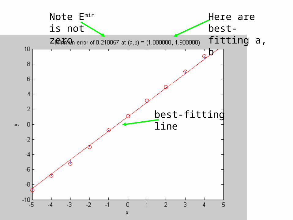
Note Emin is not zero

Here are best-fitting a, b

best-fitting line

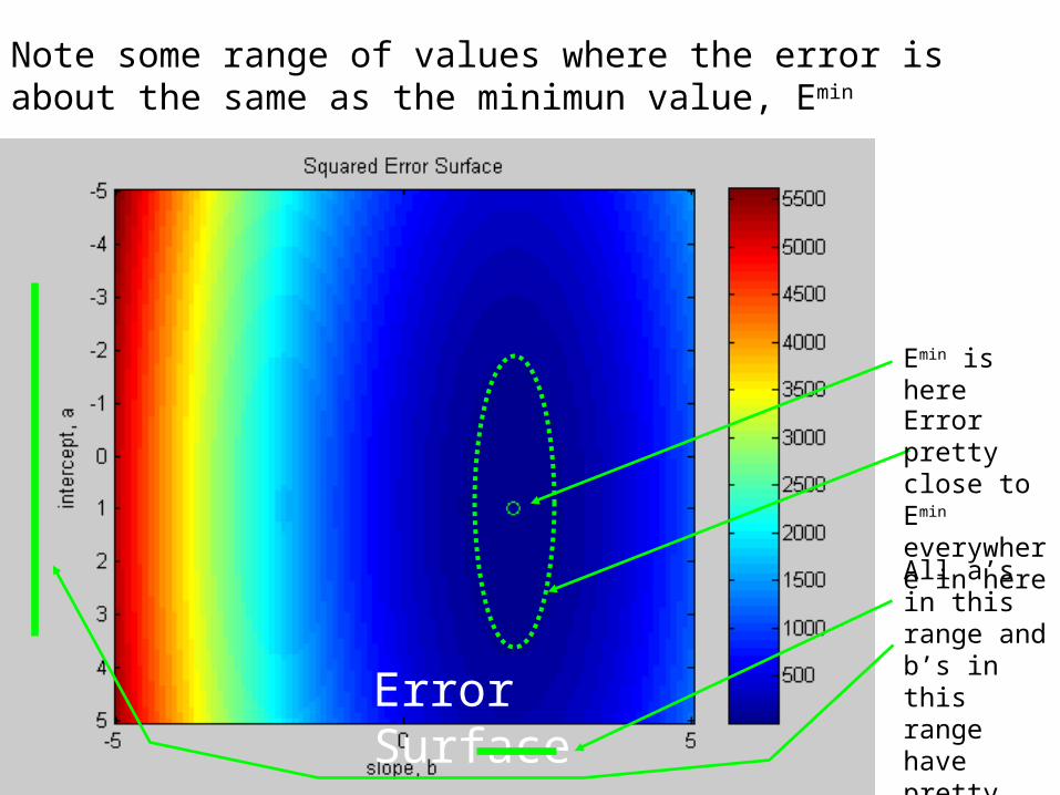
Note some range of values where the error is about the same as the minimun value, Emin

Error Surface

Emin is here

Error pretty close to Emin everywhere in here

All a’s in this range and b’s in this range have pretty much the same error

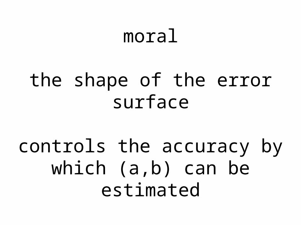
moral

the shape of the error surface

controls the accuracy by which (a,b) can be estimated

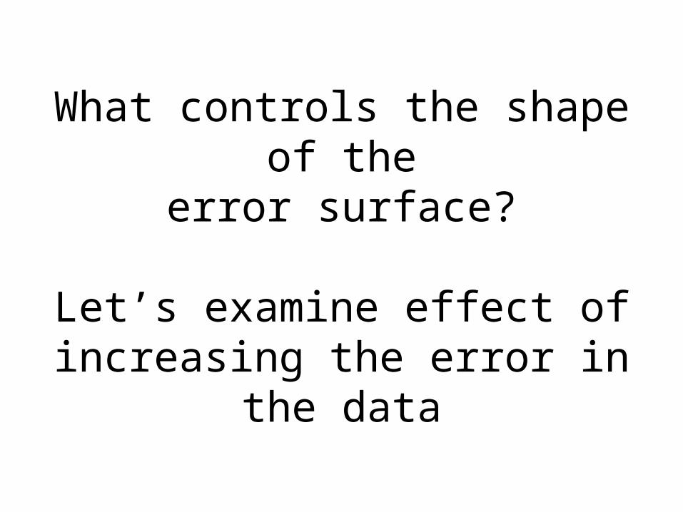
What controls the shape of theerror surface?

Let’s examine effect of increasing the error in the data

Error in data = 0.5

Error in data = 5.0

Emin = 0.20

Emin = 23.5

The minimum error increases, but the shame of the error surface is pretty much the same

What controls the shape of theerror surface?

Let’s examine effect of shifting the x-position of the data

0 105

Big change by simply shifting x-values of the data

Region of low error is now tilted

High b low a has low error

Low b high a has low error

But (high b, high a) and (low a, low b) have high error

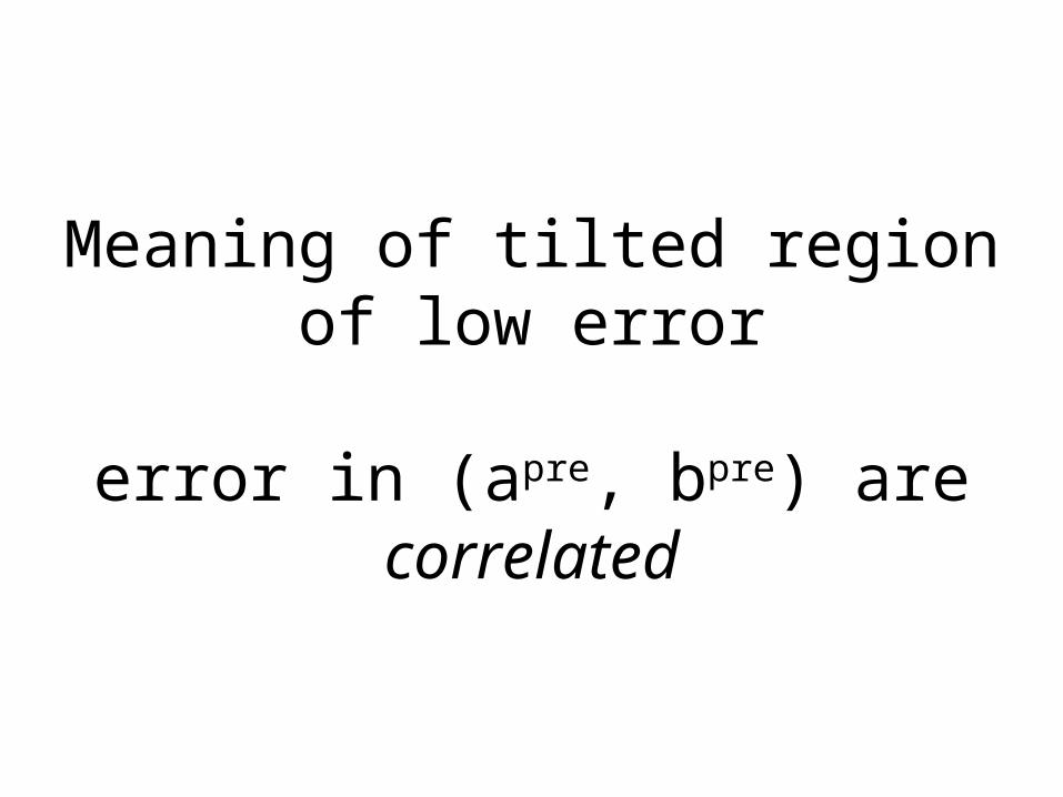
Meaning of tilted region of low error

error in (apre, bpre) arecorrelated

Best-fit

line

Best fit intercept

erroneous intercept

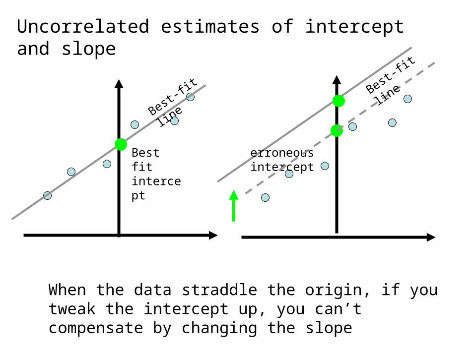
When the data straddle the origin, if you tweak the intercept up, you can’t compensate by changing the slope

Best-fit

line

Uncorrelated estimates of intercept and slope

Best-fit

line

Best fit intercept

Low slope line

erroneous intercept

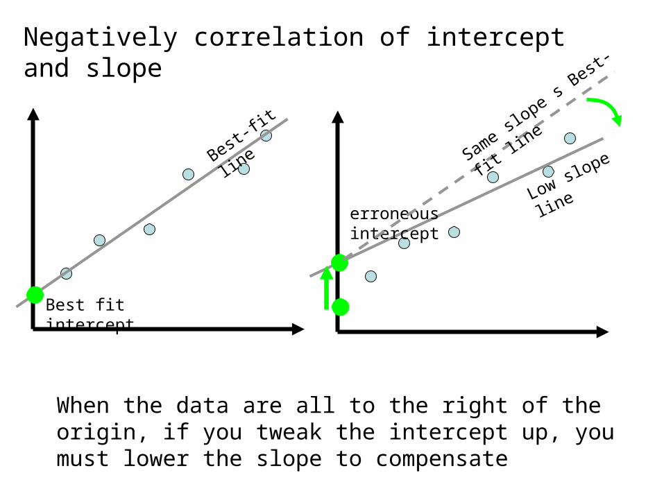
When the data are all to the right of the origin, if you tweak the intercept up, you must lower the slope to compensate

Same slope s

Best-fit

line

Negatively correlation of intercept and slope

Best-fit

line

Best fit intercept

erroneous intercept

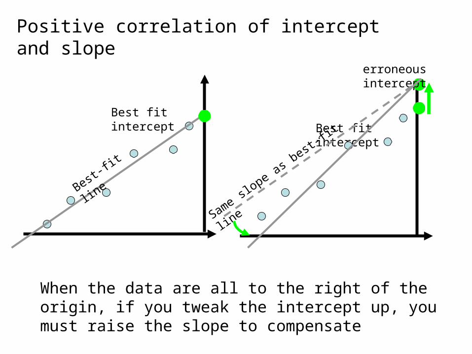
When the data are all to the right of the origin, if you tweak the intercept up, you must raise the slope to compensate

Same slope as b

est-fit

line

Positive correlation of intercept and slope

Best fit intercept

data near originpossibly good control on intercept

but lousy control on slope

-5 0 5

smal

l

big

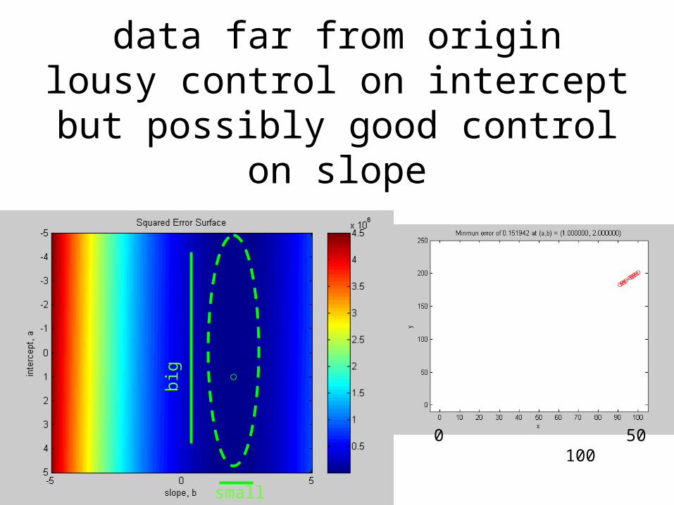
data far from originlousy control on intercept

but possibly good control on slope

small

big

0 50 100

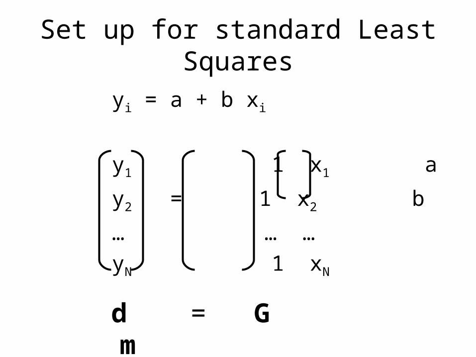
Set up for standard Least Squares

yi = a + b xi

y1 1 x1 a

y2 = 1 x2 b

… … …

yN 1 xN

d = G m

Standard Least-squares Solution

mest = [GTG]-1 GT d

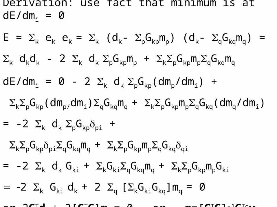
Derivation: use fact that minimum is at dE/dmi = 0

E = k ek ek = k (dk- pGkpmp) (dk- qGkqmq) =

k dkdk - 2 k dk pGkpmp + kpGkpmpqGkqmq

dE/dmi = 0 - 2 k dk pGkp(dmp/dmi) +

kpGkp(dmp/dmi)qGkqmq + kpGkpmpqGkq(dmq/dmi)

= -2 k dk pGkppi +

kpGkppiqGkqmq + kpGkpmpqGkqqi

= -2 k dk Gki + kGkiqGkqmq + kpGkpmpGki

2 k Gki dk + 2 q [kGkiGkq]mq = 0

or 2GTd + 2[GTG]m = 0 or m=[GTG]-1GTdy

Why least-squares?

Why not least-absolute length?

Or something else?

Least-Squares Least Absolute Value

a=1.00 b=2.02 a=0.94 b = 2.02