Lecture 3: Mixture Models for Microbiome data - nioo.knaw.nl · Paul J. McMurdie! w/ contribution from! Prof Susan Holmes, Stanford University Lecture 3:! Mixture Models for Microbiome

Paul J. McMurdie w/ contribution from Prof Susan Holmes, Stanford University

Lecture 3: Mixture Models for Microbiome data

1

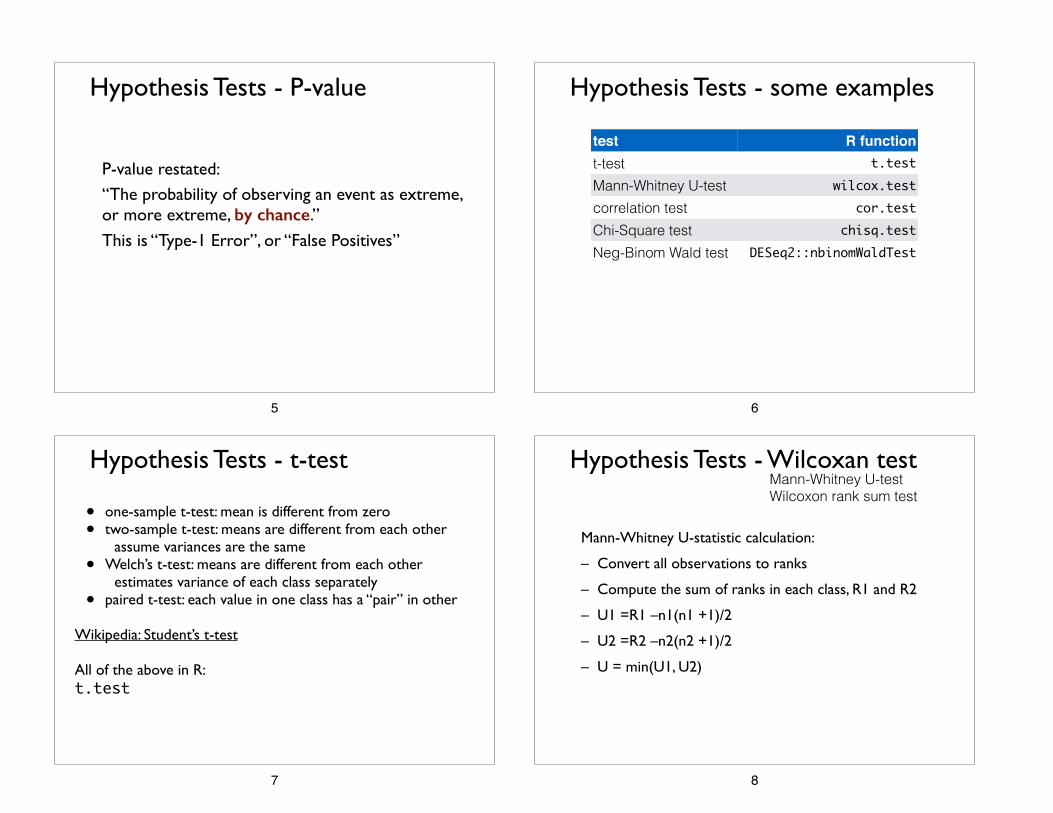
Lecture 3: Mixture Models for Microbiome data

Outline: - Hypothesis Test Intro (t, wilcoxan) - Multiple Testing (FDR) - Mixture Models (Negative Binomial) - DESeq2 / Don’t Rarefy. Ever.

2

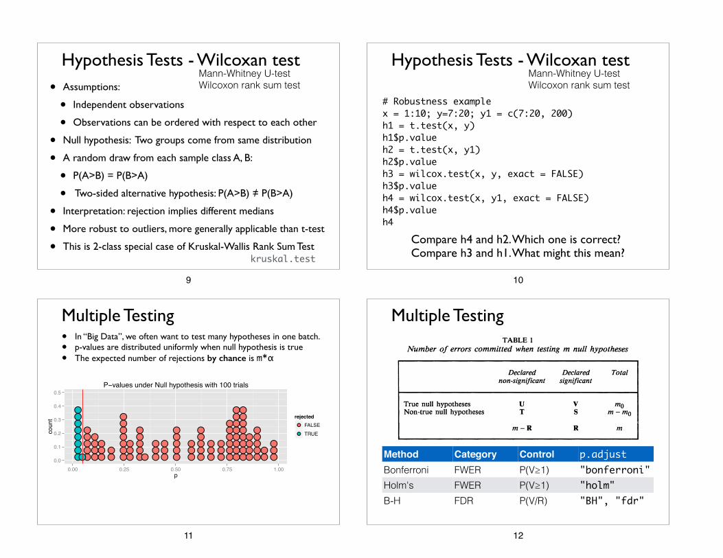
Hypothesis Tests - review

• A hypothesis is a precise disprovable statement.

• “Null hypothesis” - the default position. “Nothing special”

• Alternative/Rejection: Evidence disagrees with the Null

• Null hypothesis cannot be confirmed by the data.

3

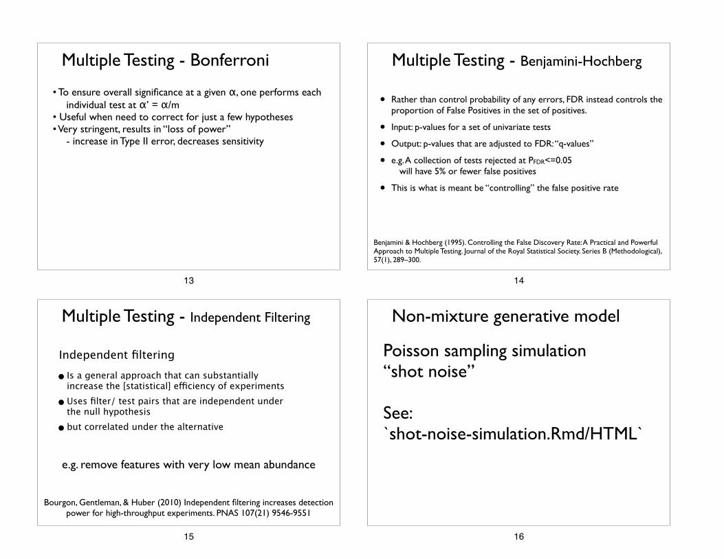
Hypothesis Tests - P-value• If the Null Hypothesis is true, then a statistic, used to

perform the test, will follow the Null distribution.

• P-value is the tail probability under the Null distribution

4

Hypothesis Tests - P-value

P-value restated: “The probability of observing an event as extreme, or more extreme, by chance.”

This is “Type-1 Error”, or “False Positives”

5

Hypothesis Tests - some examples

test R functiont-test t.testMann-Whitney U-test wilcox.testcorrelation test cor.testChi-Square test chisq.testNeg-Binom Wald test DESeq2::nbinomWaldTest

6

Hypothesis Tests - t-test

• one-sample t-test: mean is different from zero • two-sample t-test: means are different from each other assume variances are the same • Welch’s t-test: means are different from each other estimates variance of each class separately • paired t-test: each value in one class has a “pair” in other

!Wikipedia: Student’s t-test !All of the above in R: t.test

7

Mann-Whitney U-statistic calculation:

– Convert all observations to ranks

– Compute the sum of ranks in each class, R1 and R2

– U1 =R1 –n1(n1 +1)/2

– U2 =R2 –n2(n2 +1)/2

– U = min(U1, U2)

Mann-Whitney U-test Wilcoxon rank sum test

Hypothesis Tests - Wilcoxan test

8

• Assumptions:

• Independent observations

• Observations can be ordered with respect to each other

• Null hypothesis: Two groups come from same distribution

• A random draw from each sample class A, B:

• P(A>B) = P(B>A)

• Two-sided alternative hypothesis: P(A>B) = P(B>A)

• Interpretation: rejection implies different medians

• More robust to outliers, more generally applicable than t-test

• This is 2-class special case of Kruskal-Wallis Rank Sum Test



kruskal.test

9



# Robustness examplex = 1:10; y=7:20; y1 = c(7:20, 200)h1 = t.test(x, y)h1$p.valueh2 = t.test(x, y1)h2$p.valueh3 = wilcox.test(x, y, exact = FALSE)h3$p.valueh4 = wilcox.test(x, y1, exact = FALSE)h4$p.valueh4

Compare h4 and h2. Which one is correct? Compare h3 and h1. What might this mean?

10

Multiple Testing• In “Big Data”, we often want to test many hypotheses in one batch. • p-values are distributed uniformly when null hypothesis is true • The expected number of rejections by chance is m*α

●●●●●

●●●●

●●●

●●

●●●●●●●

●●●

●●●●●

● ●●●

●●●

●●●●●

●●●

●●●●●

●●●

●●●

●●●●●●

●●●●●●●●

●●●●●●●●

●●●●

●●●●●

●●

●●●

●●●●●●●●

●0.0

0.1

0.2

0.3

0.4

0.5

0.00 0.25 0.50 0.75 1.00p

coun

t rejected●

●

FALSETRUE

P−values under Null hypothesis with 100 trials

11

Multiple Testing

Method Category Control p.adjustBonferroni FWER P(V≥1) "bonferroni"Holm's FWER P(V≥1) "holm"B-H FDR P(V/R) "BH", "fdr"

12

• To ensure overall significance at a given α, one performs each individual test at α’ = α/m • Useful when need to correct for just a few hypotheses • Very stringent, results in “loss of power” - increase in Type II error, decreases sensitivity

Multiple Testing - Bonferroni

13

• Rather than control probability of any errors, FDR instead controls the proportion of False Positives in the set of positives.

• Input: p-values for a set of univariate tests

• Output: p-values that are adjusted to FDR: “q-values”

• e.g. A collection of tests rejected at PFDR<=0.05 will have 5% or fewer false positives

• This is what is meant be “controlling” the false positive rate

Multiple Testing - Benjamini-Hochberg

Benjamini & Hochberg (1995). Controlling the False Discovery Rate: A Practical and Powerful Approach to Multiple Testing. Journal of the Royal Statistical Society. Series B (Methodological), 57(1), 289–300.

14

Multiple Testing - Independent Filtering

•Is a general approach that can substantially increase the [statistical] efficiency of experiments

•Uses filter/ test pairs that are independent under the null hypothesis

•but correlated under the alternative

Bourgon, Gentleman, & Huber (2010) Independent filtering increases detection power for high-throughput experiments. PNAS 107(21) 9546-9551

Independent filtering

e.g. remove features with very low mean abundance

15

Poisson sampling simulation “shot noise” !

See: `shot-noise-simulation.Rmd/HTML` !

Non-mixture generative model

16

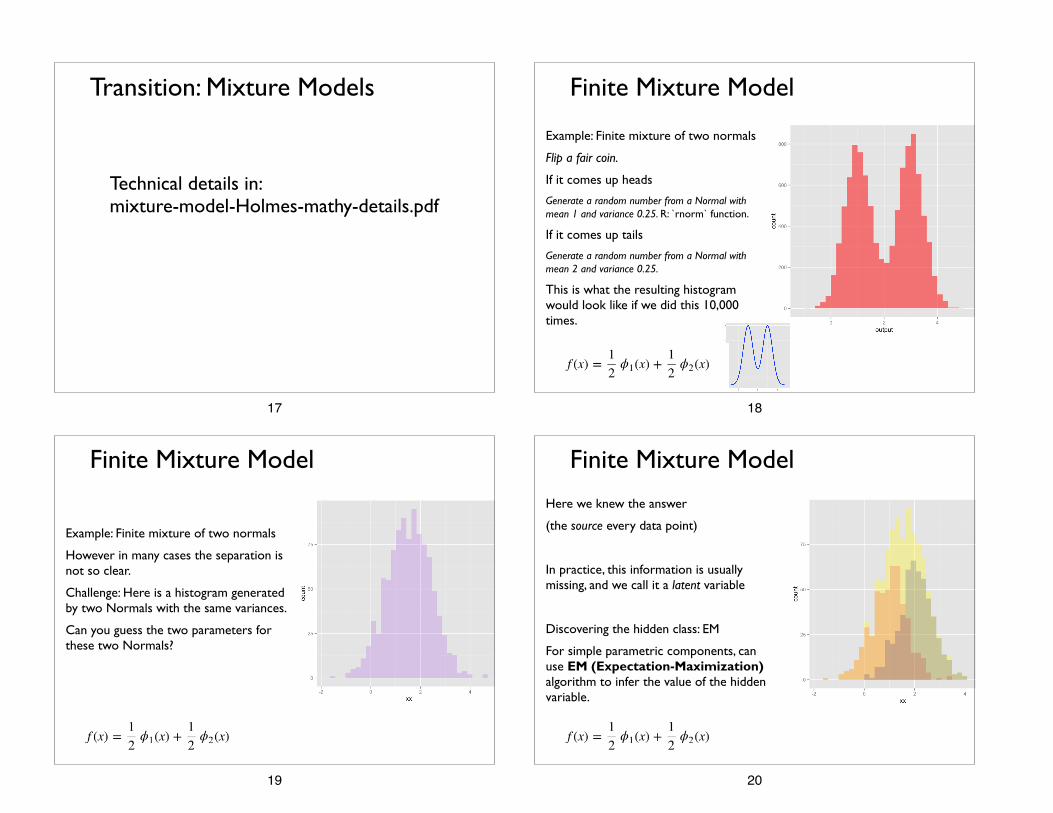
Transition: Mixture Models

Technical details in: mixture-model-Holmes-mathy-details.pdf

17

Example: Finite mixture of two normals

Flip a fair coin.

If it comes up heads

Generate a random number from a Normal with mean 1 and variance 0.25. R: `rnorm` function.

If it comes up tails

Generate a random number from a Normal with mean 2 and variance 0.25.

This is what the resulting histogram would look like if we did this 10,000 times.

Finite Mixture Model

18

Example: Finite mixture of two normals

However in many cases the separation is not so clear.

Challenge: Here is a histogram generated by two Normals with the same variances.

Can you guess the two parameters for these two Normals?


19

Here we knew the answer

(the source every data point)

!In practice, this information is usually missing, and we call it a latent variable

!Discovering the hidden class: EM

For simple parametric components, can use EM (Expectation-Maximization) algorithm to infer the value of the hidden variable.


20

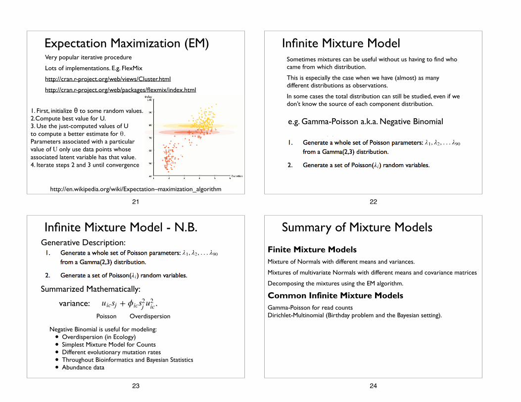
Very popular iterative procedure

Lots of implementations. E.g. FlexMix

http://cran.r-project.org/web/views/Cluster.html

http://cran.r-project.org/web/packages/flexmix/index.html

Expectation Maximization (EM)

http://en.wikipedia.org/wiki/Expectation–maximization_algorithm

1. First, initialize θ to some random values. 2.Compute best value for U. 3. Use the just-computed values of U

to compute a better estimate for θ. Parameters associated with a particular value of U only use data points whose associated latent variable has that value. 4. Iterate steps 2 and 3 until convergence

21

Infinite Mixture ModelSometimes mixtures can be useful without us having to find who came from which distribution.

This is especially the case when we have (almost) as many different distributions as observations.

In some cases the total distribution can still be studied, even if we don’t know the source of each component distribution.

e.g. Gamma-Poisson a.k.a. Negative Binomial

22

Infinite Mixture Model - N.B.Generative Description:

Negative Binomial is useful for modeling: • Overdispersion (in Ecology) • Simplest Mixture Model for Counts • Different evolutionary mutation rates • Throughout Bioinformatics and Bayesian Statistics • Abundance data

Summarized Mathematically:

variance:Poisson Overdispersion

23

Finite Mixture Models

Mixture of Normals with different means and variances.

Mixtures of multivariate Normals with different means and covariance matrices

Decomposing the mixtures using the EM algorithm.

Common Infinite Mixture Models

Gamma-Poisson for read countsDirichlet-Multinomial (Birthday problem and the Bayesian setting).

Summary of Mixture Models

24

• Modern sequencing creates libraries of unequal sizes

• Early analyses focused on library-wise distances:

paradigm: rarefy - UniFrac - PCoA - Write Paper

• This approach has “leaked” into formal settings, standard normalization method is “rarefying”

Inefficient Normalization by “rarefying”

species

samples

species counts

& applicability of Negative Binomial Mixture Model

25

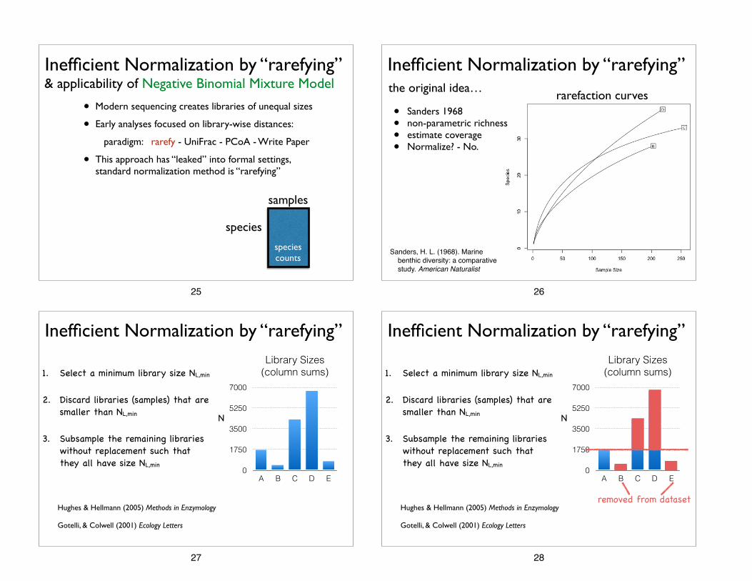
the original idea…rarefaction curves

• Sanders 1968 • non-parametric richness • estimate coverage • Normalize? - No.

Sanders, H. L. (1968). Marine benthic diversity: a comparative study. American Naturalist


26

Gotelli, & Colwell (2001) Ecology Letters

Hughes & Hellmann (2005) Methods in Enzymology

1. Select a minimum library size NL,min

2. Discard libraries (samples) that are smaller than NL,min

3. Subsample the remaining libraries without replacement such that they all have size NL,min

Library Sizes (column sums)

0

1750

3500

5250

7000

A B C D E

N


27

Gotelli, & Colwell (2001) Ecology Letters

Hughes & Hellmann (2005) Methods in Enzymology

Library Sizes (column sums)

0

1750

3500

5250

7000

A B C D E

N

removed from dataset

1. Select a minimum library size NL,min

2. Discard libraries (samples) that are smaller than NL,min

3. Subsample the remaining libraries without replacement such that they all have size NL,min


28

Microbiome Clustering Simulation

samples

OTU

s

test null

OTU

s

191163173123010

574851357899307

191163173000

000

357899307

15 15 161 0 0 0 0

87 4 72 0 0 0 0

10 148 15 0 0 0 0

0 0 0 82 244 7 24

0 0 0 354 452 92 1

0 0 0 14 9 33 251

samples

OTU

s

Ocean Feces

OTU

s

Ocean Feces

1. Sum rows. A multinomial for each sample class.

2. Deterministic mixing. Mix multinomials in precise proportion.

Ocean Feces

Microbiome Clustering Simulationsamples

OTU

s

Environment

OTU

s

1. Sum rows for each environment.

2. Sample from multinomial.

Differential Abundance Simulation

3. Multiply randomly

selected OTUs within test class by

effect size.

4. Perform differential abundance tests,

evaluate performance.

158 56 214 39 47 4 11 11 5 3

124 54 212 29 40 3 10 7 8 6

129 46 216 33 42 4 13 7 3 6

11 3 14 3 1 39 95 63 29 37

19 7 34 7 0 88 237 137 73 86

9 1 15 1 2 29 84 51 14 29

OTU

s

samples

Simulated Ocean Simulated Feces

3. Sample from these multinomials.

4. Perform clustering, evaluate accuracy.

BA

Microbiome count data from the Global

Patterns dataset

Repeat for each effect size and media library size.

Repeat for each environ-ment, number of sam-ples, effect size, and median library size.

Amount added is library size / effect size

29

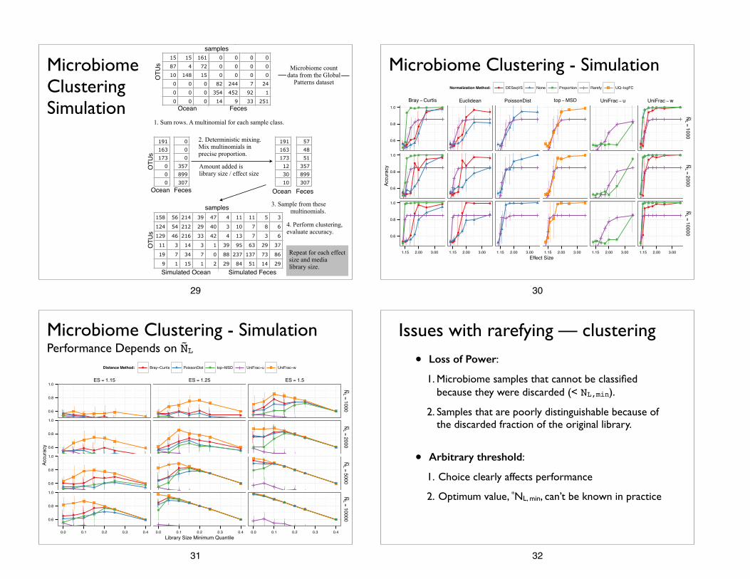
Microbiome Clustering - Simulation

Bray −Curtis Euclidean PoissonDist top −MSD UniFrac − u UniFrac −w

●●●

●●

●

●

●

●●●

●

●

●

●●

●●●

●

●

●●

●

●●●

●●

●

●●

●●●

●

●

●

● ●

●●●

●

●

● ● ●

●●

●

●●

● ● ●

●●

●

●

● ●● ●

●

●

● ● ●● ●

●

0.6

0.8

1.0

0.6

0.8

1.0

0.6

0.8

1.0

N ~L=

1000N ~

L=

2000N ~

L=

10000

1.15 2.00 3.00 1.15 2.00 3.00 1.15 2.00 3.00 1.15 2.00 3.00 1.15 2.00 3.00 1.15 2.00 3.00Effect Size

Accu

racy

Normalization Method: ● DESeqVS None Proportion Rarefy UQ−logFC

30

Performance Depends on ÑLMicrobiome Clustering - Simulation

ES = 1.15 ES = 1.25 ES = 1.5

●● ●

●●

●●

● ●●

●●

●

●

● ● ●

● ● ●

●

● ●●

● ●●

●

● ●●

●●

● ●

●

●

●●

●●

●

●●

● ●●

●

●

●

●●

●●

●

●

●

●

●

● ● ●

●

● ●

● ●●

●

●

●● ●

●

●

●

●

●●

●●

●

●

●

0.6

0.8

1.0

0.6

0.8

1.0

0.6

0.8

1.0

0.6

0.8

1.0

N ~L=

1000N ~

L=

2000N ~

L=

5000N ~

L=

10000

0.0 0.1 0.2 0.3 0.4 0.0 0.1 0.2 0.3 0.4 0.0 0.1 0.2 0.3 0.4Library Size Minimum Quantile

Accu

racy

Distance Method: ● Bray−Curtis PoissonDist top−MSD UniFrac−u UniFrac−w

31

Issues with rarefying — clustering

• Loss of Power:

1. Microbiome samples that cannot be classified because they were discarded (< NL,min).

2. Samples that are poorly distinguishable because of the discarded fraction of the original library.

• Arbitrary threshold:

1. Choice clearly affects performance

2. Optimum value, *NL, min, can’t be known in practice

32

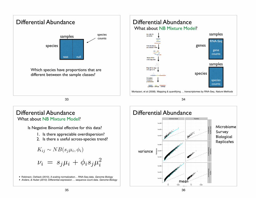
Differential Abundance

species

samples species counts

test null

Which species have proportions that are different between the sample classes?

33


Mortazavi, et al (2008). Mapping & quantifying … transcriptomes by RNA-Seq. Nature Methods

genes

samples

species

samples

RNA-Seq

species counts

gene counts

What about NB Mixture Model?

34

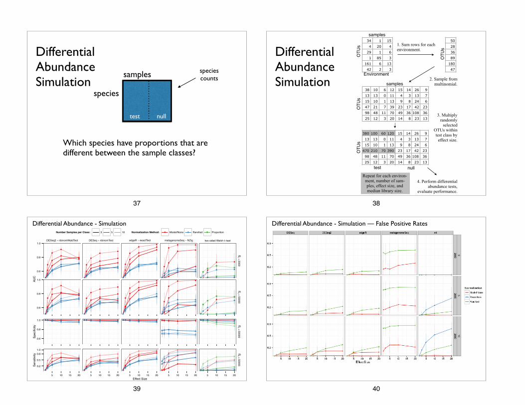
1. Is there appreciable overdispersion? 2. Is there a useful across-species trend?

2

a Poisson random variable in most cases [5]. How-ever, we are usually interested in understanding vari-ation among biological replicates, wherein a mixturemodel is necessary to account for the added uncer-tainty [6]. Taking a hierarchical model approach withthe Gamma-Poisson has provided a satisfactory fit toRNA-Seq data [7], as well as a valid regression frame-work that uses generalized linear models [8]. A Gammamixture of Poisson variables gives the negative binomial(NB) distribution [6, 7] and several RNA-Seq analysispackages now model the counts, K, for gene i, in sam-ple j according to:

Kij ⇠ NB(sjµi,�i) (1)

where sj is a linear scaling factor for sample j thataccounts for its library size, µi is the mean proportionfor gene i, and �i is the dispersion parameter for genei. The variance is ⌫i = sjµi + �isjµ

2i , with the NB

distribution becoming Poisson when � = 0. Recogniz-ing that � > 0 and estimating its value is important ingene-level tests. This reduces false positive genes thatappear significant under a Poisson distribution, but notafter accounting for non-zero dispersion.

The uncertainty in estimating �i for every gene whenthere is a small number of samples — or a small num-ber of biological replicates — can be mitigated by shar-ing information across the thousands of genes in an ex-periment, leveraging a systematic trend in the mean-dispersion relationship [7]. This approach substantiallyincreases the power to detect differences in proportions(differential expression) while still adequately control-ling for false positives [9]. Many R packages imple-menting this model of RNA-Seq data are now available,differing mainly in their approach to modeling disper-sion across genes [10].

Analogous to the development of gene expression re-search, culture independent [11] microbial ecology re-search has migrated away from detection of species (orOperational Taxonomic Units, OTUs) through microar-ray hybridization of rRNA gene PCR amplicons [12]to direct sequencing of highly-variable regions of theseamplicons [13], or even direct shotgun sequencing ofmicrobiome metagenomic DNA [14]. Although theselatter microbiome investigations use the same DNAsequencing platforms and represent the processed se-quence data in the same manner — a feature-by-samplecontingency table where the features are OTUs insteadof genes — the modeling and normalization methodsjust described for RNA-Seq analysis have not been

transferred to microbiome research [15, 16].Standard microbiome analysis workflows begin with

an ad hoc library size normalization by random subsam-pling without replacement, or so-called rarefying [17].Rarefying is most often defined by the following steps.

1. Select a minimum library size, NL.

2. Discard libraries (samples) that are smaller thanNL in size.

3. Subsample the remaining libraries without replace-ment such that they all have size NL.

Often NL is chosen to be equal to the size of the small-est library that is not considered an artifact, though inexperiments with large variation in library size iden-tifying artifact samples can be subjective. In manycases researchers have also failed to repeat the randomsubsampling step or record the pseudorandom num-ber generation seed/process – both of which are es-sential for reproducibility. To our knowledge, rare-fying was first recommended for microbiome countsin order to moderate the sensitivity of the UniFracdistance [18] to library size, especially differencesin the presence of rare OTUs attributable to librarysize [19]. In these and similar studies the principalobjective is to compare microbiome samples from dif-ferent sources, a research task that is increasingly ac-cessible with declining sequencing costs and the abilityto sequence many samples in parallel using barcodedprimers [20,21]. Rarefying is now an exceedingly com-mon precursor to microbiome multivariate workflowsthat seek to relate sample covariates to sample-wisedistance matrices [17, 22, 23]; for example, integratedas a recommended option in QIIME’s [24] beta_-diversity_through_plots.py workflow, inSub.sample in the mothur software library [25], andin daisychopper.pl [26]. This perception in themicrobiome literature of “rarefying to even samplingdepth” as a standard normalization procedure appearsto explain why rarefied counts are also used in studiesthat attempt to detect differential abundance of OTUsbetween predefined classes of samples [27–31], in addi-tion to studies that use proportions directly [32].

Statistical motivationUnfortunately, rarefying biological count data is unjus-tified despite its current ubiquity in microbiome anal-yses. The following is a minimal example to explain

2

a Poisson random variable in most cases [5]. How-ever, we are usually interested in understanding vari-ation among biological replicates, wherein a mixturemodel is necessary to account for the added uncer-tainty [6]. Taking a hierarchical model approach withthe Gamma-Poisson has provided a satisfactory fit toRNA-Seq data [7], as well as a valid regression frame-work that uses generalized linear models [8]. A Gammamixture of Poisson variables gives the negative binomial(NB) distribution [6, 7] and several RNA-Seq analysispackages now model the counts, K, for gene i, in sam-ple j according to:

Kij ⇠ NB(sjµi,�i) (1)

where sj is a linear scaling factor for sample j thataccounts for its library size, µi is the mean proportionfor gene i, and �i is the dispersion parameter for genei. The variance is ⌫i = sjµi + �isjµ

2i , with the NB

distribution becoming Poisson when � = 0. Recogniz-ing that � > 0 and estimating its value is important ingene-level tests. This reduces false positive genes thatappear significant under a Poisson distribution, but notafter accounting for non-zero dispersion.

The uncertainty in estimating �i for every gene whenthere is a small number of samples — or a small num-ber of biological replicates — can be mitigated by shar-ing information across the thousands of genes in an ex-periment, leveraging a systematic trend in the mean-dispersion relationship [7]. This approach substantiallyincreases the power to detect differences in proportions(differential expression) while still adequately control-ling for false positives [9]. Many R packages imple-menting this model of RNA-Seq data are now available,differing mainly in their approach to modeling disper-sion across genes [10].

Analogous to the development of gene expression re-search, culture independent [11] microbial ecology re-search has migrated away from detection of species (orOperational Taxonomic Units, OTUs) through microar-ray hybridization of rRNA gene PCR amplicons [12]to direct sequencing of highly-variable regions of theseamplicons [13], or even direct shotgun sequencing ofmicrobiome metagenomic DNA [14]. Although theselatter microbiome investigations use the same DNAsequencing platforms and represent the processed se-quence data in the same manner — a feature-by-samplecontingency table where the features are OTUs insteadof genes — the modeling and normalization methodsjust described for RNA-Seq analysis have not been

transferred to microbiome research [15, 16].Standard microbiome analysis workflows begin with

an ad hoc library size normalization by random subsam-pling without replacement, or so-called rarefying [17].Rarefying is most often defined by the following steps.

1. Select a minimum library size, NL.

2. Discard libraries (samples) that are smaller thanNL in size.

3. Subsample the remaining libraries without replace-ment such that they all have size NL.

Often NL is chosen to be equal to the size of the small-est library that is not considered an artifact, though inexperiments with large variation in library size iden-tifying artifact samples can be subjective. In manycases researchers have also failed to repeat the randomsubsampling step or record the pseudorandom num-ber generation seed/process – both of which are es-sential for reproducibility. To our knowledge, rare-fying was first recommended for microbiome countsin order to moderate the sensitivity of the UniFracdistance [18] to library size, especially differencesin the presence of rare OTUs attributable to librarysize [19]. In these and similar studies the principalobjective is to compare microbiome samples from dif-ferent sources, a research task that is increasingly ac-cessible with declining sequencing costs and the abilityto sequence many samples in parallel using barcodedprimers [20,21]. Rarefying is now an exceedingly com-mon precursor to microbiome multivariate workflowsthat seek to relate sample covariates to sample-wisedistance matrices [17, 22, 23]; for example, integratedas a recommended option in QIIME’s [24] beta_-diversity_through_plots.py workflow, inSub.sample in the mothur software library [25], andin daisychopper.pl [26]. This perception in themicrobiome literature of “rarefying to even samplingdepth” as a standard normalization procedure appearsto explain why rarefied counts are also used in studiesthat attempt to detect differential abundance of OTUsbetween predefined classes of samples [27–31], in addi-tion to studies that use proportions directly [32].

Statistical motivationUnfortunately, rarefying biological count data is unjus-tified despite its current ubiquity in microbiome anal-yses. The following is a minimal example to explain

Is Negative Binomial effective for this data?

Differential AbundanceWhat about NB Mixture Model?

• Robinson, Oshlack (2010). A scaling normalization… RNA-Seq data. Genome Biology!• Anders, & Huber (2010). Differential expression … sequence count data. Genome Biology

35

Common Scale Rarefied

1e+02

1e+05

1e+08

1e+02

1e+05

1e+08

1e+02

1e+05

1e+08

DietPatterns

GlobalPatterns

GlobalPatterns

2004 HighFat

freshwaterm

arine

10 1000 10 1000Mean

Varia

nce

variance

mean

Microbiome Survey Biological Replicates


36


species

samples species counts

test null

Which species have proportions that are different between the sample classes?

37


38 10 6 12 15 14 26 913 13 0 11 4 3 13 715 10 1 13 9 8 24 647 21 7 39 23 17 42 2398 48 11 70 49 36 108 3625 12 3 20 14 8 23 13

380 100 60 120 15 14 26 913 13 0 11 4 3 13 715 10 1 13 9 8 24 6470 210 70 390 23 17 42 2398 48 11 70 49 36 108 3625 12 3 20 14 8 23 13

samples

OTU

s

test null

OTU

s

5028368918047

34 1 154 20 429 1 61 85 3

161 6 1342 2 3

samples

OTU

s

Ocean Feces

OTU

s

Ocean Feces

1. Sum rows. A multinomial for each sample class.

2. Deterministic mixing. Mix multinomials in precise proportion.

Ocean Feces

Microbiome Clustering Simulationsamples

OTU

s

Environment

OTU

s

1. Sum rows for each environment.

2. Sample from multinomial.


3. Multiply randomly

selected OTUs within test class by

effect size.

4. Perform differential abundance tests,

evaluate performance.

OTU

s

samples

Simulated Ocean Simulated Feces

3. Sample from these multinomials.

4. Perform clustering, evaluate accuracy.

BA

Microbiome count data from the Global

Patterns dataset

Repeat for each effect size and media library size.

Repeat for each environ-ment, number of sam-ples, effect size, and median library size.

Amount added is library size / effect size

38

Differential Abundance - Simulation

DESeq2 − nbinomWaldTest DESeq − nbinomTest edgeR − exactTest metagenomeSeq − fitZig two sided Welch t−test

●●●

●

●

●●

●

●

●

●

●

●●●

●●●

●●

●

●

●

●

●●

●

●●●

●●●

●

●

●

●

●

●

●

●

●

●

●

●

●●●

●●

●

●

●

●

●●

●

●

●

●

●●●

●

●

● ●

●

●

●

●

●

●

●

●

●●●

●●

● ●

●

●●

●

●

●

●●

●●● ●

●

●

●

●

●

●

●

●

●

●

●

●●● ●●

●

●

●

●

●

●

●

●

●

●●●● ●●● ●●

●

●●

●

●●

●

●●● ●●● ●●

●

●●

●

●●

●

0.6

0.8

1.0

0.6

0.8

1.0

N ~L=

2000N ~

L=

50000

AUC

Number Samples per Class: 3 5 10 Normalization Method: ● Model/None Rarefied Proportion

● ● ● ● ● ● ● ● ● ● ● ● ● ● ● ● ● ● ● ● ● ● ● ● ●

0.6

0.8

1.0

N ~L=

50000Spec

ifici

ty

●

●

●

●●

●

●●

●●

●

●

●

●

●

● ●●

● ●

● ● ● ● ●

0.2

0.5

0.81.0

N ~L=

50000

5 10 15 20 5 10 15 20 5 10 15 20 5 10 15 20 5 10 15 20Effect Size

Sens

itivi

ty

39

Differential Abundance - Simulation — False Positive Rates

40

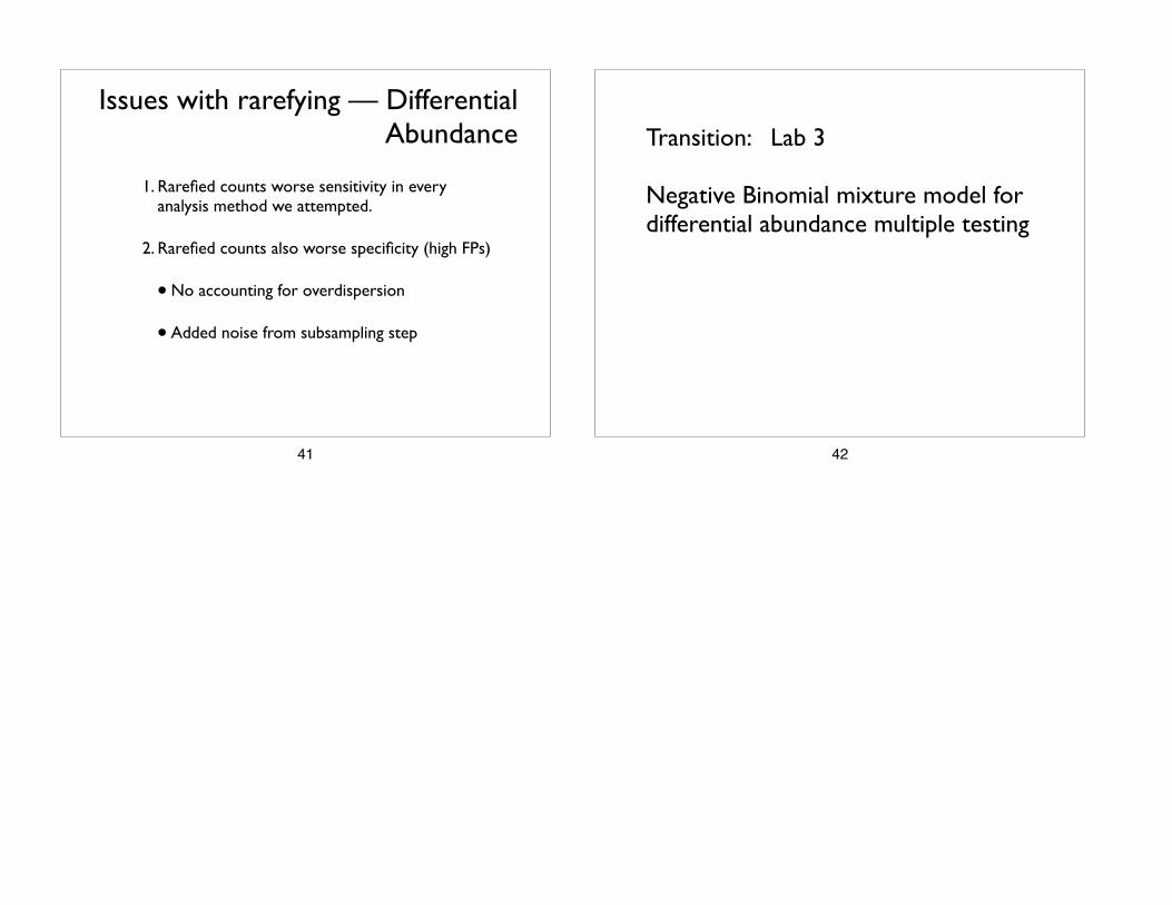
1. Rarefied counts worse sensitivity in every analysis method we attempted.

2. Rarefied counts also worse specificity (high FPs)

• No accounting for overdispersion

• Added noise from subsampling step

Issues with rarefying — Differential Abundance

41

!

Transition: Lab 3 !

Negative Binomial mixture model for differential abundance multiple testing

42

Documents

Lecture 3: Mixture Models for Microbiome data - nioo.knaw.nl · Paul J. McMurdie! w/ contribution from! Prof Susan Holmes, Stanford University Lecture 3:! Mixture Models for Microbiome