Embed Size (px)
Citation preview
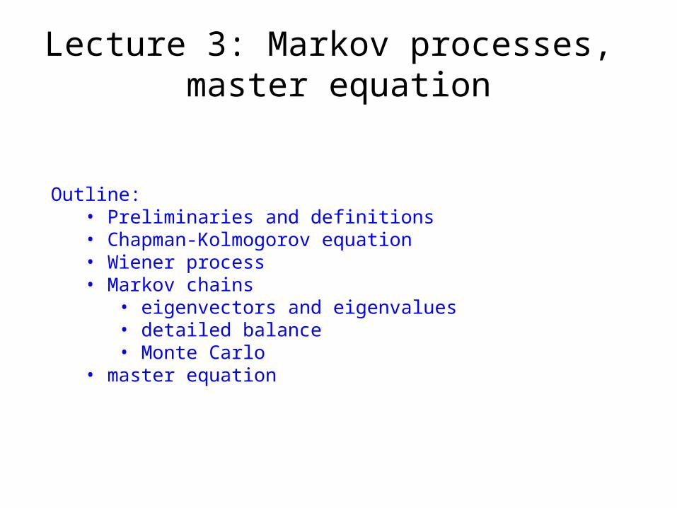
Lecture 3: Markov processes, master equation
Outline:• Preliminaries and definitions• Chapman-Kolmogorov equation• Wiener process• Markov chains
• eigenvectors and eigenvalues• detailed balance• Monte Carlo
• master equation

Stochastic processes
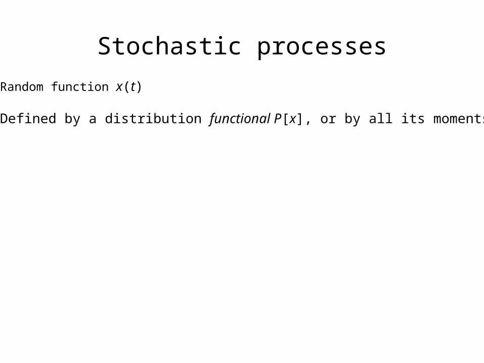
Random function x(t)
Stochastic processes
Random function x(t)
Defined by a distribution functional P[x], or by all its moments

Stochastic processes
Random function x(t)
Defined by a distribution functional P[x], or by all its moments
€
x(t) , x(t1)x(t2) , x(t1)x(t2)x(t3) , L

Stochastic processes
Random function x(t)
Defined by a distribution functional P[x], or by all its moments
or by its characteristic functional:
€
x(t) , x(t1)x(t2) , x(t1)x(t2)x(t3) , L
€
G[k] = exp i k(t)x(t)dt∫( )
Stochastic processes
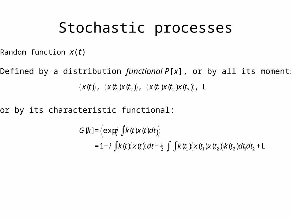
Random function x(t)
Defined by a distribution functional P[x], or by all its moments
or by its characteristic functional:
€
x(t) , x(t1)x(t2) , x(t1)x(t2)x(t3) , L
€
G[k] = exp i k(t)x(t)dt∫( )
=1− i k(t) x(t) dt∫ − 12 k(t1) x(t1)x(t2)∫∫ k(t2)dt1dt2 +L

Stochastic processes (2)
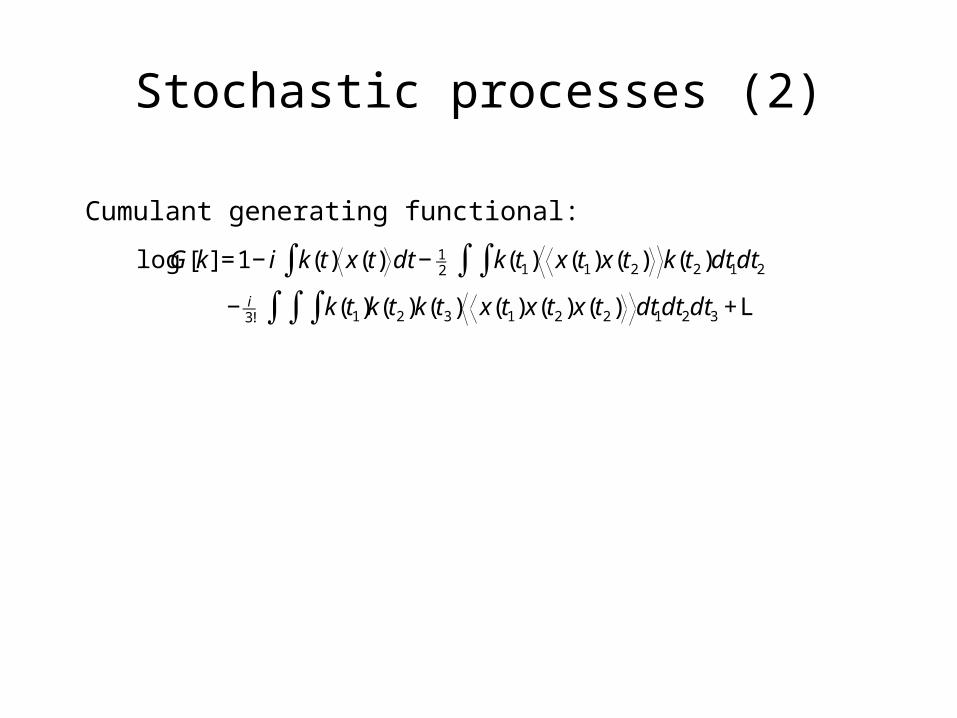
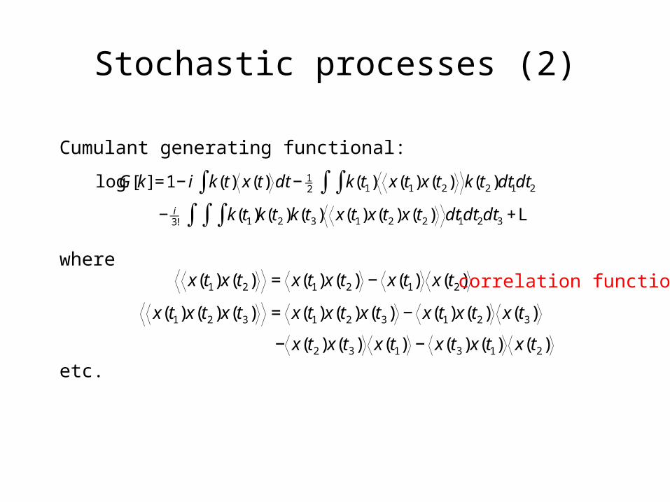
Cumulant generating functional:
Stochastic processes (2)
Cumulant generating functional:
€
logG[k] =1− i k(t) x(t) dt∫ − 12 k(t1) x(t1)x(t2)∫∫ k(t2)dt1dt2
− i3! k(t1)∫ k(t2)k(t3) x(t1)x(t2)x(t2)∫∫ dt1dt2dt3 +L
Stochastic processes (2)
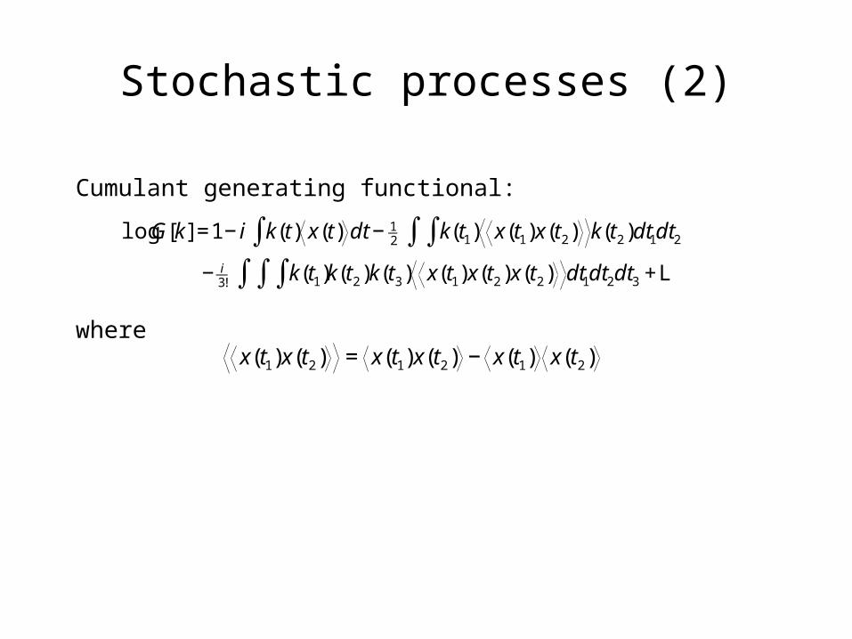
Cumulant generating functional:
where
€
logG[k] =1− i k(t) x(t) dt∫ − 12 k(t1) x(t1)x(t2)∫∫ k(t2)dt1dt2
− i3! k(t1)∫ k(t2)k(t3) x(t1)x(t2)x(t2)∫∫ dt1dt2dt3 +L
€
x(t1)x(t2) = x(t1)x(t2) − x(t1) x(t2)

Stochastic processes (2)
Cumulant generating functional:
where
€
logG[k] =1− i k(t) x(t) dt∫ − 12 k(t1) x(t1)x(t2)∫∫ k(t2)dt1dt2
− i3! k(t1)∫ k(t2)k(t3) x(t1)x(t2)x(t2)∫∫ dt1dt2dt3 +L
€
x(t1)x(t2) = x(t1)x(t2) − x(t1) x(t2) correlation function
Stochastic processes (2)
Cumulant generating functional:
where
etc.
€
logG[k] =1− i k(t) x(t) dt∫ − 12 k(t1) x(t1)x(t2)∫∫ k(t2)dt1dt2
− i3! k(t1)∫ k(t2)k(t3) x(t1)x(t2)x(t2)∫∫ dt1dt2dt3 +L
€
x(t1)x(t2) = x(t1)x(t2) − x(t1) x(t2)
x(t1)x(t2)x(t3) = x(t1)x(t2)x(t3) − x(t1)x(t2) x(t3)
− x(t2)x(t3) x(t1) − x(t3)x(t1) x(t2)
correlation function

Stochastic processes (3)
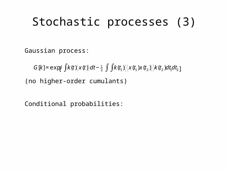
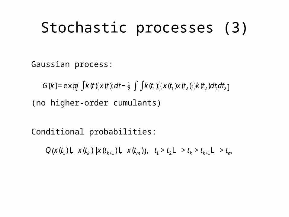
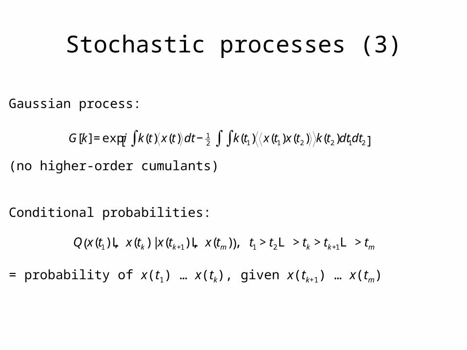
Gaussian process:

Stochastic processes (3)
Gaussian process:
€
G[k] = exp i k(t) x(t) dt∫ − 12 k(t1) x(t1)x(t2)∫∫ k(t2)dt1dt2[ ]

Stochastic processes (3)
Gaussian process:
(no higher-order cumulants)
€
G[k] = exp i k(t) x(t) dt∫ − 12 k(t1) x(t1)x(t2)∫∫ k(t2)dt1dt2[ ]
Stochastic processes (3)
Gaussian process:
(no higher-order cumulants)
Conditional probabilities:
€
G[k] = exp i k(t) x(t) dt∫ − 12 k(t1) x(t1)x(t2)∫∫ k(t2)dt1dt2[ ]
Stochastic processes (3)
Gaussian process:
(no higher-order cumulants)
Conditional probabilities:
€
G[k] = exp i k(t) x(t) dt∫ − 12 k(t1) x(t1)x(t2)∫∫ k(t2)dt1dt2[ ]
€
Q x(t1),L x(tk ) | x(tk +1),L x(tm )( ), t1 > t2L > tk > tk +1L > tm
Stochastic processes (3)
Gaussian process:
(no higher-order cumulants)
Conditional probabilities:
= probability of x(t1) … x(tk), given x(tk+1) … x(tm)
€
G[k] = exp i k(t) x(t) dt∫ − 12 k(t1) x(t1)x(t2)∫∫ k(t2)dt1dt2[ ]
€
Q x(t1),L x(tk ) | x(tk +1),L x(tm )( ), t1 > t2L > tk > tk +1L > tm

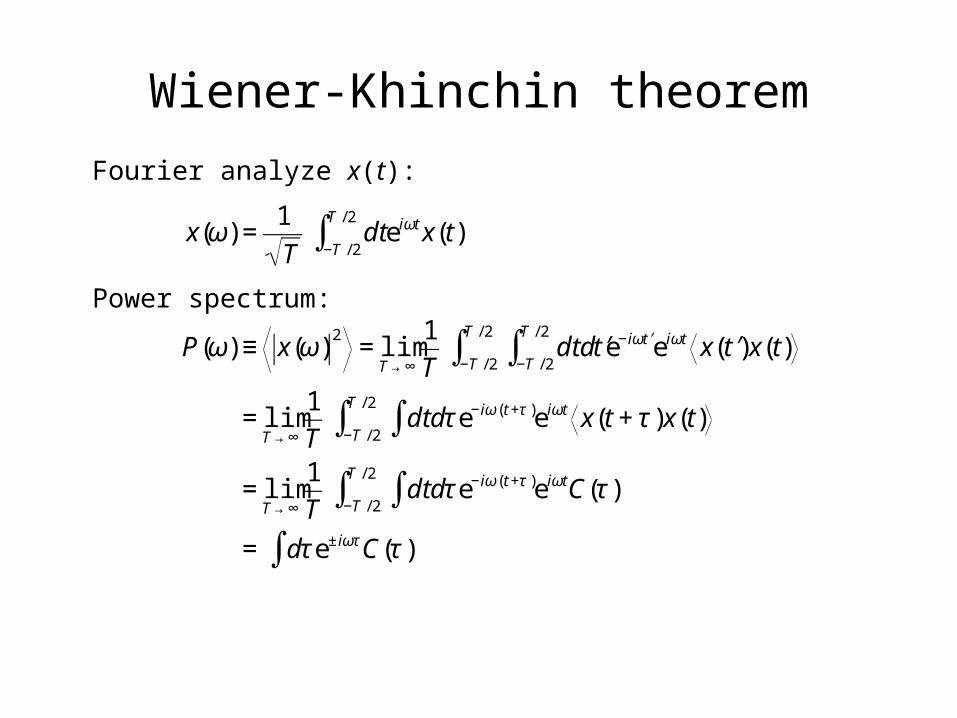
Wiener-Khinchin theorem
Fourier analyze x(t):
€
x(ω) =1
Tdt
−T / 2
T / 2
∫ e iωt x(t)

Wiener-Khinchin theorem
Fourier analyze x(t):
Power spectrum:
€
x(ω) =1
Tdt
−T / 2
T / 2
∫ e iωt x(t)
P(ω) ≡ x(ω)2

Wiener-Khinchin theorem
Fourier analyze x(t):
Power spectrum:
€
x(ω) =1
Tdt
−T / 2
T / 2
∫ e iωt x(t)
P(ω) ≡ x(ω)2
= limT →∞
1
Tdtd ′ t
−T / 2
T / 2
∫−T / 2
T / 2
∫ e−iω ′ t e iωt x( ′ t )x(t)

Wiener-Khinchin theorem
Fourier analyze x(t):
Power spectrum:
€
x(ω) =1
Tdt
−T / 2
T / 2
∫ e iωt x(t)
P(ω) ≡ x(ω)2
= limT →∞
1
Tdtd ′ t
−T / 2
T / 2
∫−T / 2
T / 2
∫ e−iω ′ t e iωt x( ′ t )x(t)
= limT →∞
1
Tdtdτ∫ e−iω(t +τ )e iωt x(t + τ )x(t)
−T / 2
T / 2
∫

Wiener-Khinchin theorem
Fourier analyze x(t):
Power spectrum:
€
x(ω) =1
Tdt
−T / 2
T / 2
∫ e iωt x(t)
P(ω) ≡ x(ω)2
= limT →∞
1
Tdtd ′ t
−T / 2
T / 2
∫−T / 2
T / 2
∫ e−iω ′ t e iωt x( ′ t )x(t)
= limT →∞
1
Tdtdτ∫ e−iω(t +τ )e iωt x(t + τ )x(t)
−T / 2
T / 2
∫
= limT →∞
1
Tdtdτ∫ e−iω(t +τ )e iωtC(τ )
−T / 2
T / 2
∫
Wiener-Khinchin theorem
Fourier analyze x(t):
Power spectrum:
€
x(ω) =1
Tdt
−T / 2
T / 2
∫ e iωt x(t)
P(ω) ≡ x(ω)2
= limT →∞
1
Tdtd ′ t
−T / 2
T / 2
∫−T / 2
T / 2
∫ e−iω ′ t e iωt x( ′ t )x(t)
= limT →∞
1
Tdtdτ∫ e−iω(t +τ )e iωt x(t + τ )x(t)
−T / 2
T / 2
∫
= limT →∞
1
Tdtdτ∫ e−iω(t +τ )e iωtC(τ )
−T / 2
T / 2
∫= dτ∫ e± iωτ C(τ )

Wiener-Khinchin theorem
Fourier analyze x(t):
Power spectrum:
Power spectrum is Fourier transform of the correlation function
€
x(ω) =1
Tdt
−T / 2
T / 2
∫ e iωt x(t)
P(ω) ≡ x(ω)2
= limT →∞
1
Tdtd ′ t
−T / 2
T / 2
∫−T / 2
T / 2
∫ e−iω ′ t e iωt x( ′ t )x(t)
= limT →∞
1
Tdtdτ∫ e−iω(t +τ )e iωt x(t + τ )x(t)
−T / 2
T / 2
∫
= limT →∞
1
Tdtdτ∫ e−iω(t +τ )e iωtC(τ )
−T / 2
T / 2
∫= dτ∫ e± iωτ C(τ )

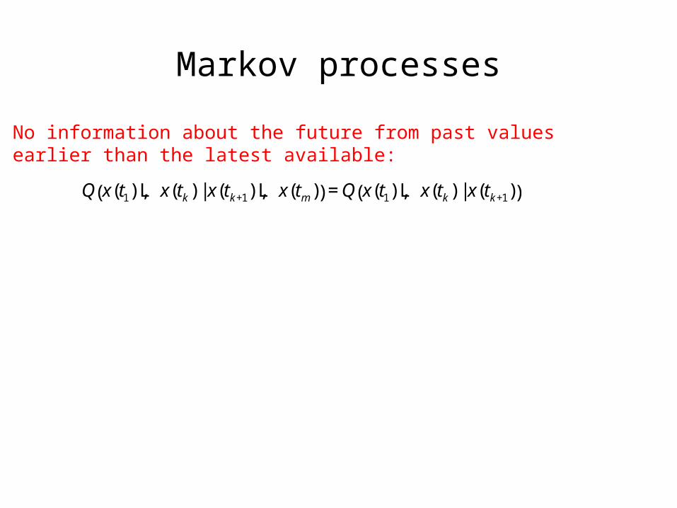
Markov processes
No information about the future from past values earlier than the latest available:
Markov processes
No information about the future from past values earlier than the latest available:
€
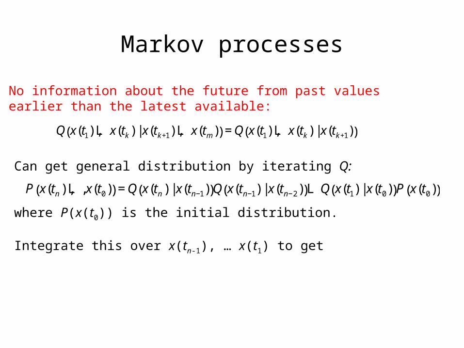
Q x(t1),L x(tk ) | x(tk +1),L x(tm )( ) = Q x(t1),L x(tk ) | x(tk +1)( )

Markov processes
No information about the future from past values earlier than the latest available:
€
Q x(t1),L x(tk ) | x(tk +1),L x(tm )( ) = Q x(t1),L x(tk ) | x(tk +1)( )
Can get general distribution by iterating Q:

Markov processes
No information about the future from past values earlier than the latest available:
€
Q x(t1),L x(tk ) | x(tk +1),L x(tm )( ) = Q x(t1),L x(tk ) | x(tk +1)( )
Can get general distribution by iterating Q:
€
P x(tn ),L ,x(t0)( ) = Q x(tn ) | x(tn−1)( )Q x(tn−1) | x(tn−2)( )L Q x(t1) | x(t0)( )P x(t0)( )

Markov processes
No information about the future from past values earlier than the latest available:
€
Q x(t1),L x(tk ) | x(tk +1),L x(tm )( ) = Q x(t1),L x(tk ) | x(tk +1)( )
Can get general distribution by iterating Q:
where P(x(t0)) is the initial distribution.
€
P x(tn ),L ,x(t0)( ) = Q x(tn ) | x(tn−1)( )Q x(tn−1) | x(tn−2)( )L Q x(t1) | x(t0)( )P x(t0)( )
Markov processes
No information about the future from past values earlier than the latest available:
€
Q x(t1),L x(tk ) | x(tk +1),L x(tm )( ) = Q x(t1),L x(tk ) | x(tk +1)( )
Can get general distribution by iterating Q:
where P(x(t0)) is the initial distribution.
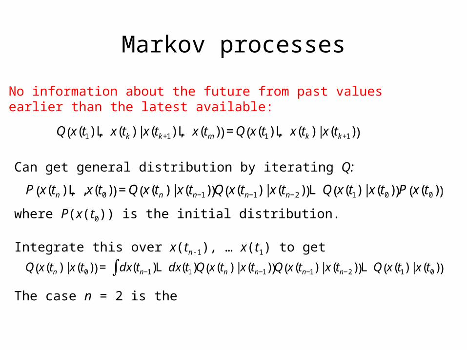
Integrate this over x(tn-1), … x(t1) to get
€
P x(tn ),L ,x(t0)( ) = Q x(tn ) | x(tn−1)( )Q x(tn−1) | x(tn−2)( )L Q x(t1) | x(t0)( )P x(t0)( )

Markov processes
No information about the future from past values earlier than the latest available:
€
Q x(t1),L x(tk ) | x(tk +1),L x(tm )( ) = Q x(t1),L x(tk ) | x(tk +1)( )
Can get general distribution by iterating Q:
where P(x(t0)) is the initial distribution.
Integrate this over x(tn-1), … x(t1) to get
€
P x(tn ),L ,x(t0)( ) = Q x(tn ) | x(tn−1)( )Q x(tn−1) | x(tn−2)( )L Q x(t1) | x(t0)( )P x(t0)( )
€
Q x(tn ) | x(t0)( ) = dx(tn−1)L dx(t1∫ )Q x(tn ) | x(tn−1)( )Q x(tn−1) | x(tn−2)( )L Q x(t1) | x(t0)( )
Markov processes
No information about the future from past values earlier than the latest available:
€
Q x(t1),L x(tk ) | x(tk +1),L x(tm )( ) = Q x(t1),L x(tk ) | x(tk +1)( )
Can get general distribution by iterating Q:
where P(x(t0)) is the initial distribution.
Integrate this over x(tn-1), … x(t1) to get
The case n = 2 is the
€
P x(tn ),L ,x(t0)( ) = Q x(tn ) | x(tn−1)( )Q x(tn−1) | x(tn−2)( )L Q x(t1) | x(t0)( )P x(t0)( )
€
Q x(tn ) | x(t0)( ) = dx(tn−1)L dx(t1∫ )Q x(tn ) | x(tn−1)( )Q x(tn−1) | x(tn−2)( )L Q x(t1) | x(t0)( )

Chapman-Kolmogorov equation
€
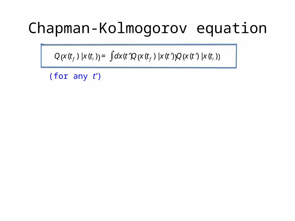
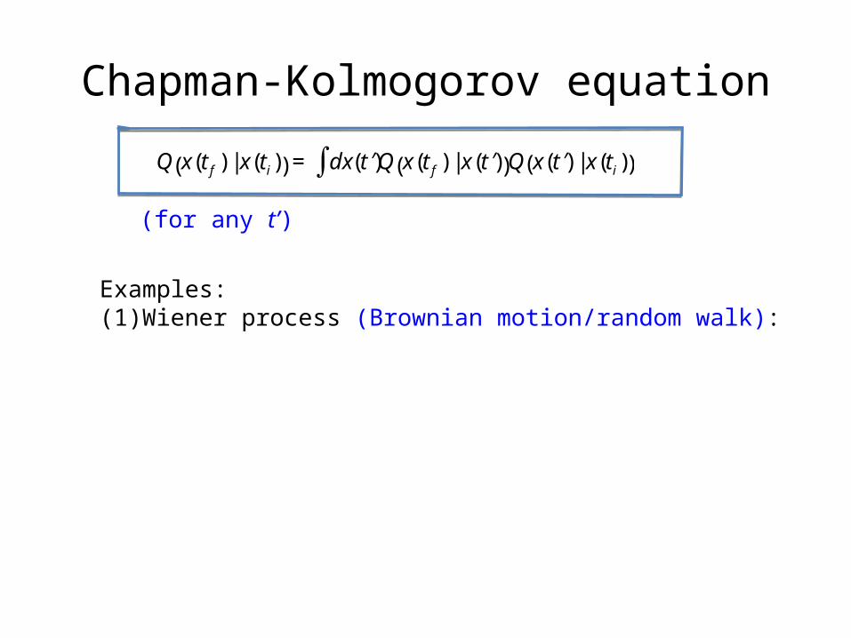
Q x(t f ) | x(ti)( ) = dx( ′ t )∫ Q x(t f ) | x( ′ t )( )Q x( ′ t ) | x(ti)( )

Chapman-Kolmogorov equation
€
Q x(t f ) | x(ti)( ) = dx( ′ t )∫ Q x(t f ) | x( ′ t )( )Q x( ′ t ) | x(ti)( )
Chapman-Kolmogorov equation
€
Q x(t f ) | x(ti)( ) = dx( ′ t )∫ Q x(t f ) | x( ′ t )( )Q x( ′ t ) | x(ti)( )
(for any t’)
Chapman-Kolmogorov equation
€
Q x(t f ) | x(ti)( ) = dx( ′ t )∫ Q x(t f ) | x( ′ t )( )Q x( ′ t ) | x(ti)( )
(for any t’)
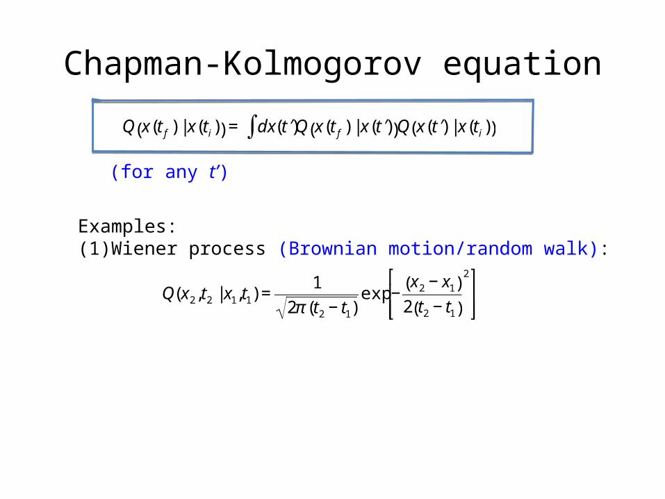
Examples: (1)Wiener process (Brownian motion/random walk):
Chapman-Kolmogorov equation
€
Q x(t f ) | x(ti)( ) = dx( ′ t )∫ Q x(t f ) | x( ′ t )( )Q x( ′ t ) | x(ti)( )
(for any t’)
Examples: (1)Wiener process (Brownian motion/random walk):
€
Q(x2, t2 | x1, t1) =1
2π (t2 − t1)exp −
x2 − x1( )2 t2 − t1( )
2 ⎡
⎣ ⎢ ⎢
⎤
⎦ ⎥ ⎥

Chapman-Kolmogorov equation
€
Q x(t f ) | x(ti)( ) = dx( ′ t )∫ Q x(t f ) | x( ′ t )( )Q x( ′ t ) | x(ti)( )
(for any t’)
Examples: (1)Wiener process (Brownian motion/random walk):
(2)(cumulative) Poisson process
€
Q(x2, t2 | x1, t1) =1
2π (t2 − t1)exp −
x2 − x1( )2 t2 − t1( )
2 ⎡
⎣ ⎢ ⎢
⎤
⎦ ⎥ ⎥
€
Q(n2, t2 | n1, t1) =t2 − t1( )
n2 −n1
n2 − n1( )!e−(t2 −t1 )

Markov chains
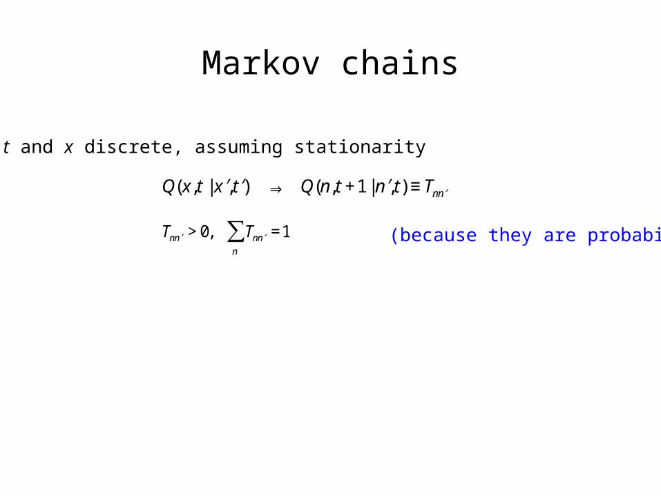
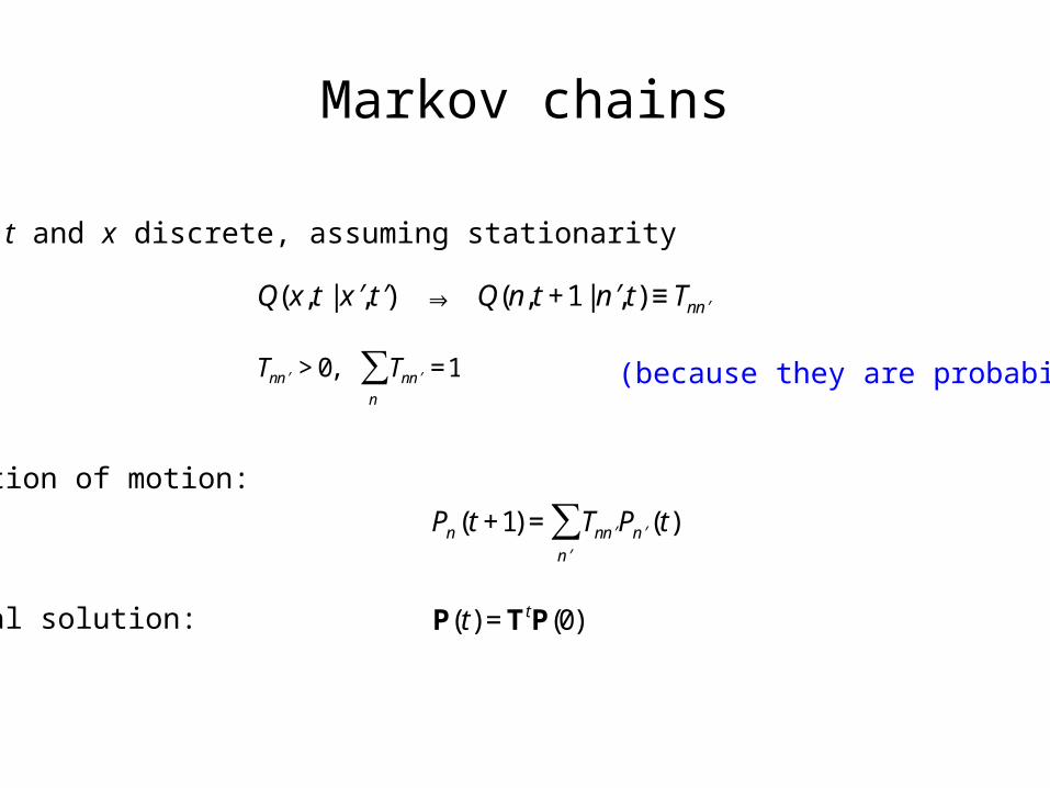
Both t and x discrete, assuming stationarity
€
Q(x, t | ′ x , ′ t ) ⇒ Q(n, t +1 | ′ n , t) ≡ Tn ′ n

Markov chains
Both t and x discrete, assuming stationarity
€
Q(x, t | ′ x , ′ t ) ⇒ Q(n, t +1 | ′ n , t) ≡ Tn ′ n
€
Tn ′ n > 0, Tn ′ n
n
∑ =1
Markov chains
Both t and x discrete, assuming stationarity
(because they are probabilities)
€
Q(x, t | ′ x , ′ t ) ⇒ Q(n, t +1 | ′ n , t) ≡ Tn ′ n
€
Tn ′ n > 0, Tn ′ n
n
∑ =1

Markov chains
Both t and x discrete, assuming stationarity
(because they are probabilities)
Equation of motion:
€
Q(x, t | ′ x , ′ t ) ⇒ Q(n, t +1 | ′ n , t) ≡ Tn ′ n
€
Pn (t +1) = Tn ′ n ′ n
∑ P ′ n (t)€
Tn ′ n > 0, Tn ′ n
n
∑ =1
Markov chains
Both t and x discrete, assuming stationarity
(because they are probabilities)
Equation of motion:
Formal solution:
€
Q(x, t | ′ x , ′ t ) ⇒ Q(n, t +1 | ′ n , t) ≡ Tn ′ n
€
Pn (t +1) = Tn ′ n ′ n
∑ P ′ n (t)
€
P(t) =TtP(0)
€
Tn ′ n > 0, Tn ′ n
n
∑ =1
Markov chains (2): properties of T
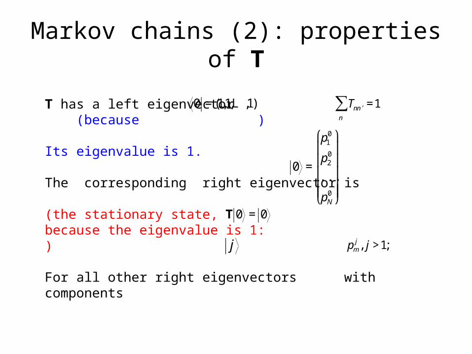
T has a left eigenvector
€
0 = (1,1,L ,1)
Markov chains (2): properties of T
T has a left eigenvector (because )
€
0 = (1,1,L ,1)
€
Tn ′ n
n
∑ =1
Markov chains (2): properties of T
T has a left eigenvector (because )
Its eigenvalue is 1.
€
0 = (1,1,L ,1)
€
Tn ′ n
n
∑ =1

Markov chains (2): properties of T
T has a left eigenvector (because )
Its eigenvalue is 1.
The corresponding right eigenvector is
€
0 =
p10
p20
...
pN0
⎛
⎝
⎜ ⎜ ⎜ ⎜ ⎜
⎞
⎠
⎟ ⎟ ⎟ ⎟ ⎟
€
0 = (1,1,L ,1)
€
Tn ′ n
n
∑ =1

Markov chains (2): properties of T
T has a left eigenvector (because )
Its eigenvalue is 1.
The corresponding right eigenvector is
(the stationary state, because the eigenvalue is 1: )
€
0 =
p10
p20
...
pN0
⎛
⎝
⎜ ⎜ ⎜ ⎜ ⎜
⎞
⎠
⎟ ⎟ ⎟ ⎟ ⎟
€
0 = (1,1,L ,1)
€
Tn ′ n
n
∑ =1
€
T 0 = 0
Markov chains (2): properties of T
T has a left eigenvector (because )
Its eigenvalue is 1.
The corresponding right eigenvector is
(the stationary state, because the eigenvalue is 1: )
For all other right eigenvectors with components
€
0 =
p10
p20
...
pN0
⎛
⎝
⎜ ⎜ ⎜ ⎜ ⎜
⎞
⎠
⎟ ⎟ ⎟ ⎟ ⎟
€
0 = (1,1,L ,1)
€
pmj , j >1;
€
j
€
Tn ′ n
n
∑ =1
€
T 0 = 0

Markov chains (2): properties of T
T has a left eigenvector (because )
Its eigenvalue is 1.
The corresponding right eigenvector is
(the stationary state, because the eigenvalue is 1: )
For all other right eigenvectors with components
€
0 =
p10
p20
...
pN0
⎛
⎝
⎜ ⎜ ⎜ ⎜ ⎜
⎞
⎠
⎟ ⎟ ⎟ ⎟ ⎟
€
0 = (1,1,L ,1)
€
pmj , j >1; pm
j
m
∑ = 0
€
j
€
Tn ′ n
n
∑ =1
€
T 0 = 0

Markov chains (2): properties of T
T has a left eigenvector (because )
Its eigenvalue is 1.
The corresponding right eigenvector is
(the stationary state, because the eigenvalue is 1: )
For all other right eigenvectors with components
(because they must be orthogonal to : )
€
0 =
p10
p20
...
pN0
⎛
⎝
⎜ ⎜ ⎜ ⎜ ⎜
⎞
⎠
⎟ ⎟ ⎟ ⎟ ⎟
€
0 = (1,1,L ,1)
€
pmj , j >1; pm
j
m
∑ = 0
€
0
€
j
€
0 j = 0
€
Tn ′ n
n
∑ =1
€
T 0 = 0

Markov chains (2): properties of T
T has a left eigenvector (because )
Its eigenvalue is 1.
The corresponding right eigenvector is
(the stationary state, because the eigenvalue is 1: )
For all other right eigenvectors with components
(because they must be orthogonal to : )
All other eigenvalues are < 1.
€
0 =
p10
p20
...
pN0
⎛
⎝
⎜ ⎜ ⎜ ⎜ ⎜
⎞
⎠
⎟ ⎟ ⎟ ⎟ ⎟
€
0 = (1,1,L ,1)
€
pmj , j >1; pm
j
m
∑ = 0
€
0
€
j
€
0 j = 0
€
Tn ′ n
n
∑ =1
€
T 0 = 0

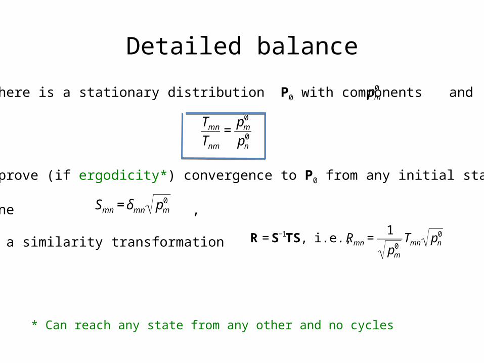
Detailed balance
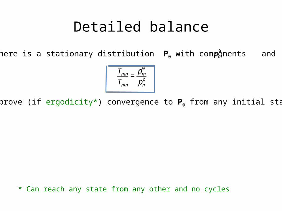
If there is a stationary distribution P0 with components and
€
pm0

Detailed balance
If there is a stationary distribution P0 with components and
€
Tmn
Tnm
=pm
0
pn0
€
pm0

Detailed balance
If there is a stationary distribution P0 with components and
€
Tmn
Tnm
=pm
0
pn0
€
pm0

Detailed balance
If there is a stationary distribution P0 with components and
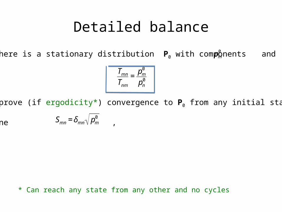
can prove (if ergodicity*) convergence to P0 from any initial state:
€
Tmn
Tnm
=pm
0
pn0
€
pm0
Detailed balance
If there is a stationary distribution P0 with components and
can prove (if ergodicity*) convergence to P0 from any initial state:
€
Tmn
Tnm
=pm
0
pn0
€
pm0
* Can reach any state from any other and no cycles
Detailed balance
If there is a stationary distribution P0 with components and
can prove (if ergodicity*) convergence to P0 from any initial state:
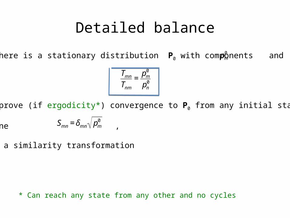
Define ,
€
Tmn
Tnm
=pm
0
pn0
€
pm0
* Can reach any state from any other and no cycles
€
Smn = δmn pm0
Detailed balance
If there is a stationary distribution P0 with components and
can prove (if ergodicity*) convergence to P0 from any initial state:
Define ,
make a similarity transformation
€
Tmn
Tnm
=pm
0
pn0
€
pm0
* Can reach any state from any other and no cycles
€
Smn = δmn pm0
Detailed balance
If there is a stationary distribution P0 with components and
can prove (if ergodicity*) convergence to P0 from any initial state:
Define ,
make a similarity transformation
€
Tmn
Tnm
=pm
0
pn0
€
pm0
* Can reach any state from any other and no cycles
€
Smn = δmn pm0
€
R = S−1TS, i.e., Rmn =1
pm0
Tmn pn0

Detailed balance
If there is a stationary distribution P0 with components and
can prove (if ergodicity*) convergence to P0 from any initial state:
Define ,
make a similarity transformation
R is symmetric, has complete set of eigenvectors , components(Eigenvalues λj same as those of T.)
€
Tmn
Tnm
=pm
0
pn0
€
pm0
* Can reach any state from any other and no cycles
€
Smn = δmn pm0
€
R = S−1TS, i.e., Rmn =1
pm0
Tmn pn0
€
qmj
€
q j
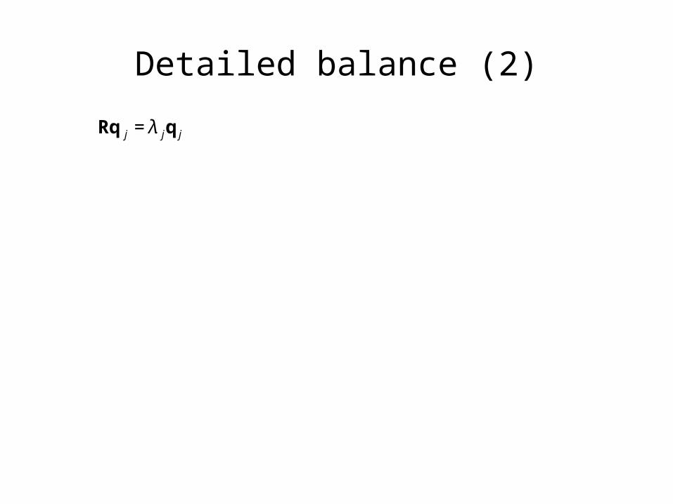
Detailed balance (2)
€
Rq j = λ jq j
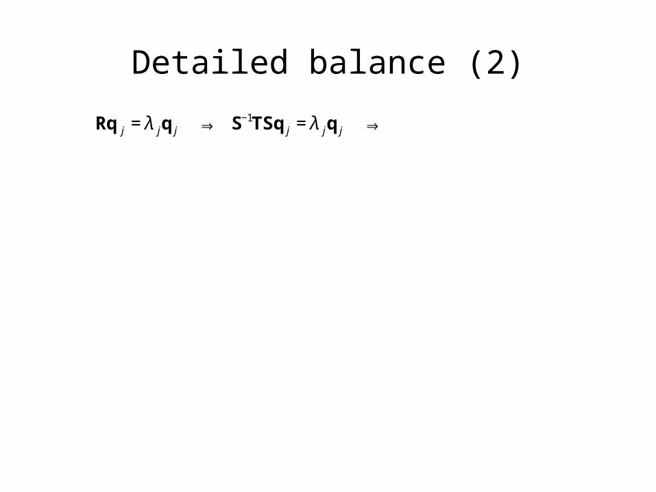
Detailed balance (2)
€
Rq j = λ jq j ⇒ S−1TSq j = λ jq j ⇒
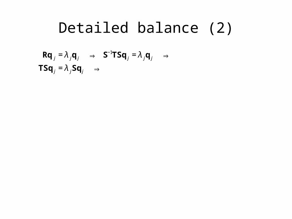
Detailed balance (2)
€
Rq j = λ jq j ⇒ S−1TSq j = λ jq j ⇒
TSq j = λ jSq j ⇒
Detailed balance (2)
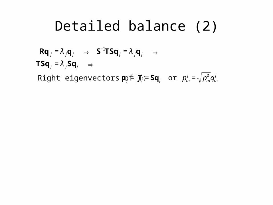
Right eigenvectors of T:
€
p j = j = Sq j or pmj = pm
0 qmj
€
Rq j = λ jq j ⇒ S−1TSq j = λ jq j ⇒
TSq j = λ jSq j ⇒

Detailed balance (2)
Right eigenvectors of T:
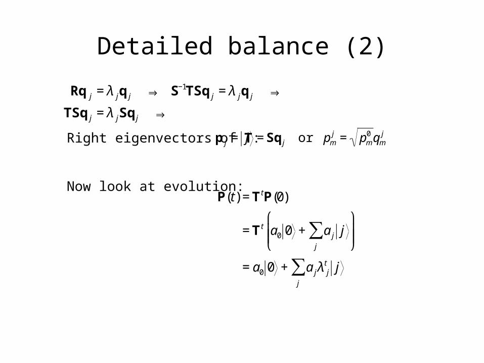
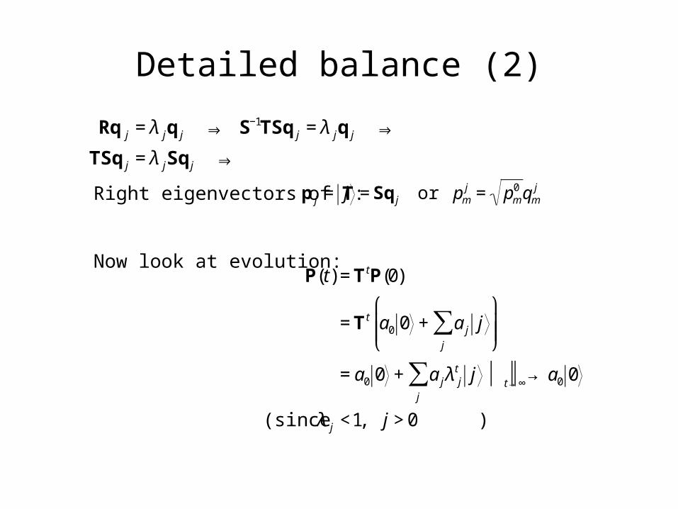
Now look at evolution:
€
p j = j = Sq j or pmj = pm
0 qmj
€
Rq j = λ jq j ⇒ S−1TSq j = λ jq j ⇒
TSq j = λ jSq j ⇒
€
P(t) =TtP(0)

Detailed balance (2)
Right eigenvectors of T:
Now look at evolution:
€
p j = j = Sq j or pmj = pm
0 qmj
€
Rq j = λ jq j ⇒ S−1TSq j = λ jq j ⇒
TSq j = λ jSq j ⇒
€
P(t) =TtP(0)
=Tt a0 0 + a j jj
∑ ⎛
⎝ ⎜ ⎜
⎞
⎠ ⎟ ⎟
Detailed balance (2)
Right eigenvectors of T:
Now look at evolution:
€
p j = j = Sq j or pmj = pm
0 qmj
€
Rq j = λ jq j ⇒ S−1TSq j = λ jq j ⇒
TSq j = λ jSq j ⇒
€
P(t) =TtP(0)
=Tt a0 0 + a j jj
∑ ⎛
⎝ ⎜ ⎜
⎞
⎠ ⎟ ⎟
= a0 0 + a jλ jt j
j
∑

Detailed balance (2)
Right eigenvectors of T:
Now look at evolution:
€
p j = j = Sq j or pmj = pm
0 qmj
€
Rq j = λ jq j ⇒ S−1TSq j = λ jq j ⇒
TSq j = λ jSq j ⇒
€
P(t) =TtP(0)
=Tt a0 0 + a j jj
∑ ⎛
⎝ ⎜ ⎜
⎞
⎠ ⎟ ⎟
= a0 0 + a jλ jt j
j
∑ t →∞ ⏐ → ⏐ ⏐ a0 0
Detailed balance (2)
Right eigenvectors of T:
Now look at evolution:
(since )
€
p j = j = Sq j or pmj = pm
0 qmj
€
Rq j = λ jq j ⇒ S−1TSq j = λ jq j ⇒
TSq j = λ jSq j ⇒
€
P(t) =TtP(0)
=Tt a0 0 + a j jj
∑ ⎛
⎝ ⎜ ⎜
⎞
⎠ ⎟ ⎟
= a0 0 + a jλ jt j
j
∑ t →∞ ⏐ → ⏐ ⏐ a0 0
λ j <1, j > 0

Detailed balance (2)
Right eigenvectors of T:
Now look at evolution:
(since )
€
p j = j = Sq j or pmj = pm
0 qmj
€
Rq j = λ jq j ⇒ S−1TSq j = λ jq j ⇒
TSq j = λ jSq j ⇒
€
P(t) =TtP(0)
=Tt a0 0 + a j jj
∑ ⎛
⎝ ⎜ ⎜
⎞
⎠ ⎟ ⎟
= a0 0 + a jλ jt j
j
∑ t →∞ ⏐ → ⏐ ⏐ a0 0 = 0
λ j <1, j > 0

Monte Carlo
72
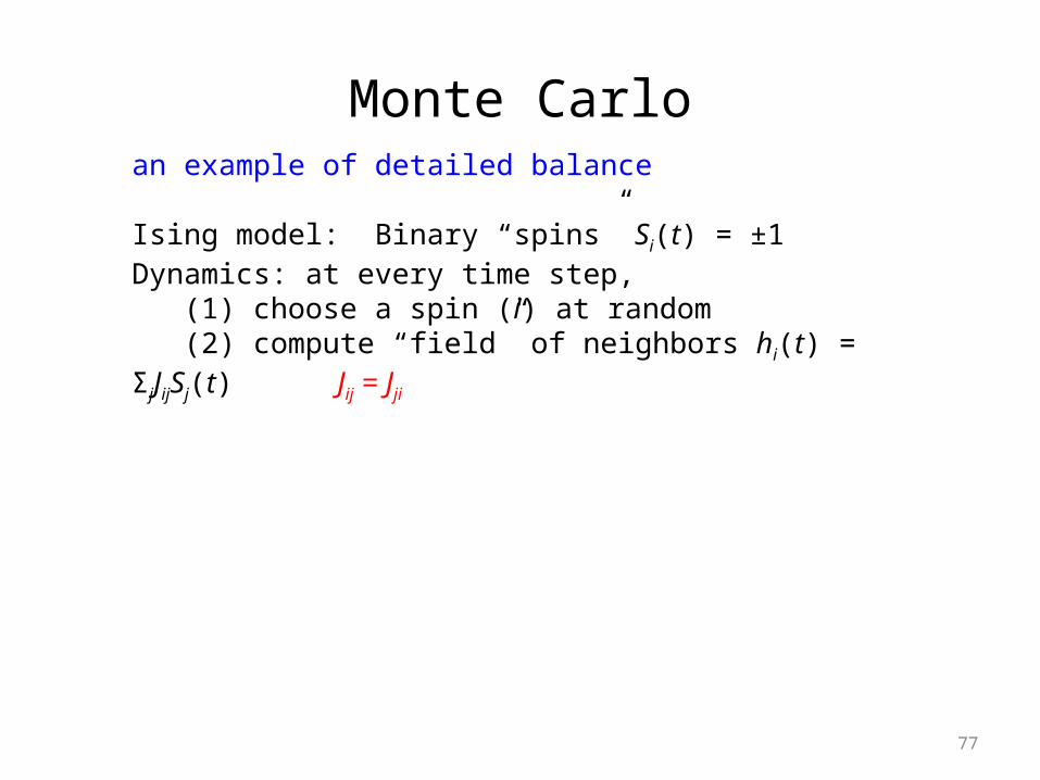
an example of detailed balance

Monte Carlo
73
an example of detailed balance
Ising model: Binary “spins” Si(t) = ±1

Monte Carlo
74
an example of detailed balance
Ising model: Binary “spins” Si(t) = ±1Dynamics: at every time step,

Monte Carlo
75
an example of detailed balance
Ising model: Binary “spins” Si(t) = ±1Dynamics: at every time step,
(1) choose a spin (i) at random

Monte Carlo
76
an example of detailed balance
Ising model: Binary “spins” Si(t) = ±1Dynamics: at every time step,
(1) choose a spin (i) at random(2) compute “field” of neighbors hi(t) = ΣjJijSj(t)
Monte Carlo
77
an example of detailed balance
Ising model: Binary “spins” Si(t) = ±1Dynamics: at every time step,
(1) choose a spin (i) at random(2) compute “field” of neighbors hi(t) = ΣjJijSj(t) Jij = Jji

Monte Carlo
78
an example of detailed balance
Ising model: Binary “spins” Si(t) = ±1Dynamics: at every time step,
(1) choose a spin (i) at random(2) compute “field” of neighbors hi(t) = ΣjJijSj(t) Jij = Jji (3) Si(t + Δt) = +1 with probability
€
P(hi) =exp βhi( )
exp βhi( ) + exp −βhi( )

Monte Carlo
79
an example of detailed balance
Ising model: Binary “spins” Si(t) = ±1Dynamics: at every time step,
(1) choose a spin (i) at random(2) compute “field” of neighbors hi(t) = ΣjJijSj(t) Jij = Jji (3) Si(t + Δt) = +1 with probability
€
P(hi) =exp βhi( )
exp βhi( ) + exp −βhi( )=
1
1+ exp(−2βhi)

Monte Carlo
80
an example of detailed balance
Ising model: Binary “spins” Si(t) = ±1Dynamics: at every time step,
(1) choose a spin (i) at random(2) compute “field” of neighbors hi(t) = ΣjJijSj(t) Jij = Jji (3) Si(t + Δt) = +1 with probability
€
P(hi) =exp βhi( )
exp βhi( ) + exp −βhi( )=
1
1+ exp(−2βhi)
Monte Carlo
81
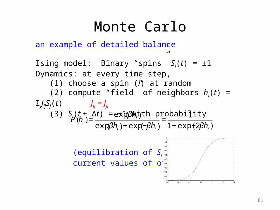
an example of detailed balance
Ising model: Binary “spins” Si(t) = ±1Dynamics: at every time step,
(1) choose a spin (i) at random(2) compute “field” of neighbors hi(t) = ΣjJijSj(t) Jij = Jji (3) Si(t + Δt) = +1 with probability
(equilibration of Si, given current values of other S’s)
€
P(hi) =exp βhi( )
exp βhi( ) + exp −βhi( )=
1
1+ exp(−2βhi)
Monte Carlo (2)
In language of Markov chains, states (n) are
€
S = (S1,S2,L ,SN )

Monte Carlo (2)
In language of Markov chains, states (n) areSingle-spin flips: transitions only between neighboring pointson hypercube
€
S = (S1,S2,L ,SN )

Monte Carlo (2)
In language of Markov chains, states (n) areSingle-spin flips: transitions only between neighboring pointson hypercube
€
S = (S1,S2,L ,SN )
€
+ = S1,S2,L Si−1,+1,Si+1,L ,SN( )
− = S1,S2,L Si−1,−1,Si+1,L ,SN( )

Monte Carlo (2)
In language of Markov chains, states (n) areSingle-spin flips: transitions only between neighboring pointson hypercube
T matrix elements:
€
S = (S1,S2,L ,SN )
€
+ = S1,S2,L Si−1,+1,Si+1,L ,SN( )
− = S1,S2,L Si−1,−1,Si+1,L ,SN( )
€
+ T + + T −
− T + − T −
⎛
⎝ ⎜ ⎜
⎞
⎠ ⎟ ⎟=
exp βhi( )exp βhi( ) + exp −βhi( )
exp βhi( )exp βhi( ) + exp −βhi( )
exp −βhi( )exp βhi( ) + exp −βhi( )
exp −βhi( )exp βhi( ) + exp −βhi( )
⎛
⎝
⎜ ⎜ ⎜ ⎜
⎞
⎠
⎟ ⎟ ⎟ ⎟

Monte Carlo (2)
In language of Markov chains, states (n) areSingle-spin flips: transitions only between neighboring pointson hypercube
T matrix elements:
all other Tmn = 0.
€
S = (S1,S2,L ,SN )
€
+ = S1,S2,L Si−1,+1,Si+1,L ,SN( )
− = S1,S2,L Si−1,−1,Si+1,L ,SN( )
€
+ T + + T −
− T + − T −
⎛
⎝ ⎜ ⎜
⎞
⎠ ⎟ ⎟=
exp βhi( )exp βhi( ) + exp −βhi( )
exp βhi( )exp βhi( ) + exp −βhi( )
exp −βhi( )exp βhi( ) + exp −βhi( )
exp −βhi( )exp βhi( ) + exp −βhi( )
⎛
⎝
⎜ ⎜ ⎜ ⎜
⎞
⎠
⎟ ⎟ ⎟ ⎟
Monte Carlo (2)
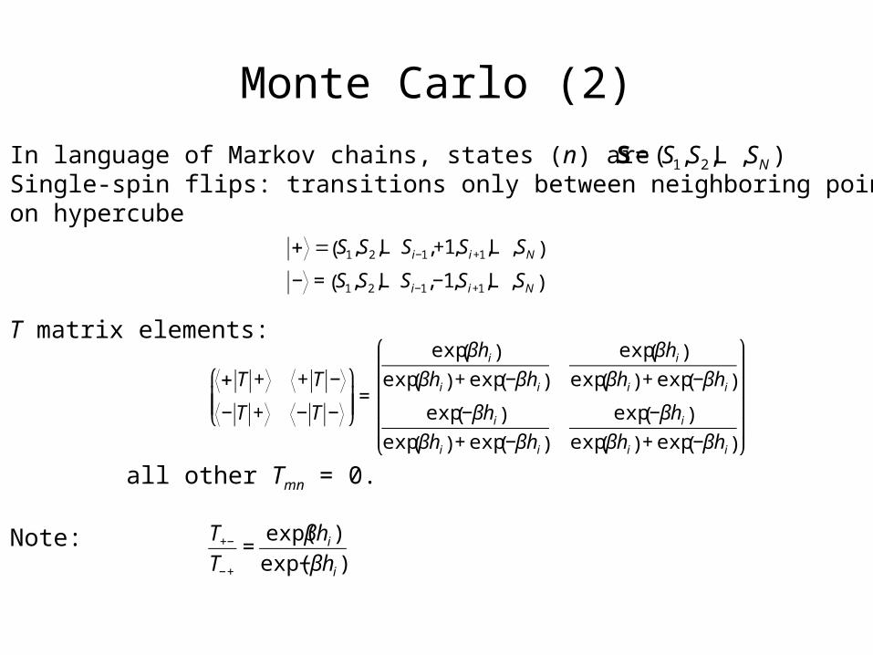
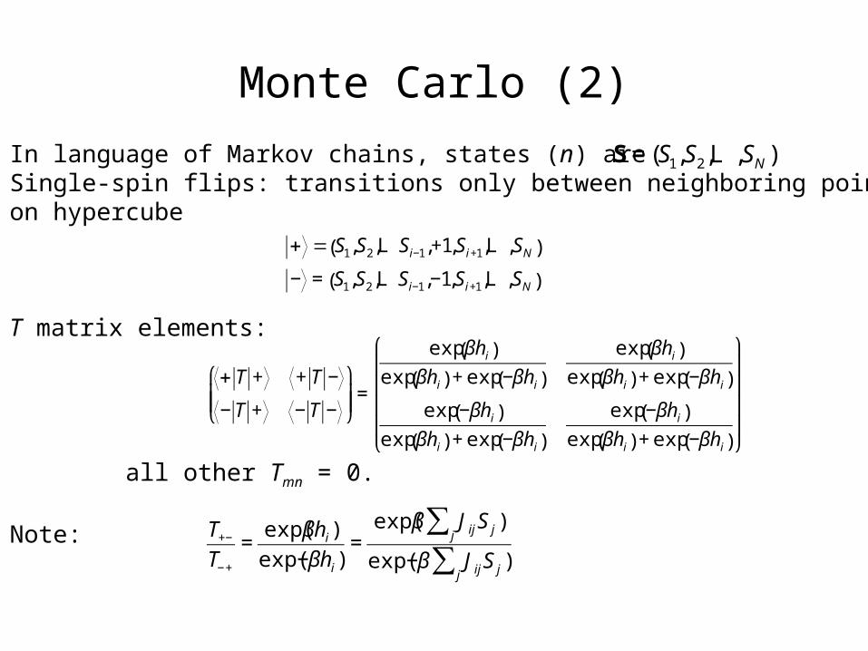
In language of Markov chains, states (n) areSingle-spin flips: transitions only between neighboring pointson hypercube
T matrix elements:
all other Tmn = 0.
Note:
€
S = (S1,S2,L ,SN )
€
+ = S1,S2,L Si−1,+1,Si+1,L ,SN( )
− = S1,S2,L Si−1,−1,Si+1,L ,SN( )
€
+ T + + T −
− T + − T −
⎛
⎝ ⎜ ⎜
⎞
⎠ ⎟ ⎟=
exp βhi( )exp βhi( ) + exp −βhi( )
exp βhi( )exp βhi( ) + exp −βhi( )
exp −βhi( )exp βhi( ) + exp −βhi( )
exp −βhi( )exp βhi( ) + exp −βhi( )
⎛
⎝
⎜ ⎜ ⎜ ⎜
⎞
⎠
⎟ ⎟ ⎟ ⎟
€
T+−
T−+
=exp(βhi)
exp(−βhi)
Monte Carlo (2)
In language of Markov chains, states (n) areSingle-spin flips: transitions only between neighboring pointson hypercube
T matrix elements:
all other Tmn = 0.
Note:
€
S = (S1,S2,L ,SN )
€
+ = S1,S2,L Si−1,+1,Si+1,L ,SN( )
− = S1,S2,L Si−1,−1,Si+1,L ,SN( )
€
+ T + + T −
− T + − T −
⎛
⎝ ⎜ ⎜
⎞
⎠ ⎟ ⎟=
exp βhi( )exp βhi( ) + exp −βhi( )
exp βhi( )exp βhi( ) + exp −βhi( )
exp −βhi( )exp βhi( ) + exp −βhi( )
exp −βhi( )exp βhi( ) + exp −βhi( )
⎛
⎝
⎜ ⎜ ⎜ ⎜
⎞
⎠
⎟ ⎟ ⎟ ⎟
€
T+−
T−+
=exp(βhi)
exp(−βhi)=
exp(β JijS jj∑ )
exp(−β JijS jj∑ )
Monte Carlo (3)
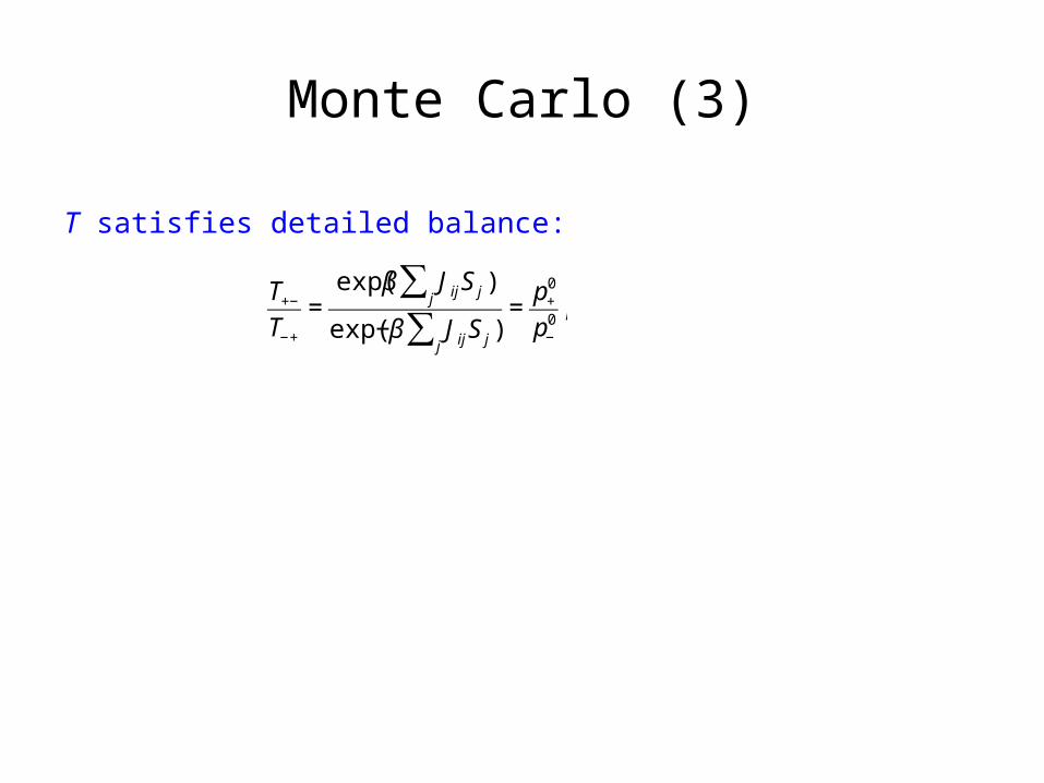
T satisfies detailed balance:
€
T+−
T−+
=exp(β JijS jj
∑ )
exp(−β JijS jj∑ )
=p+
0
p−0,
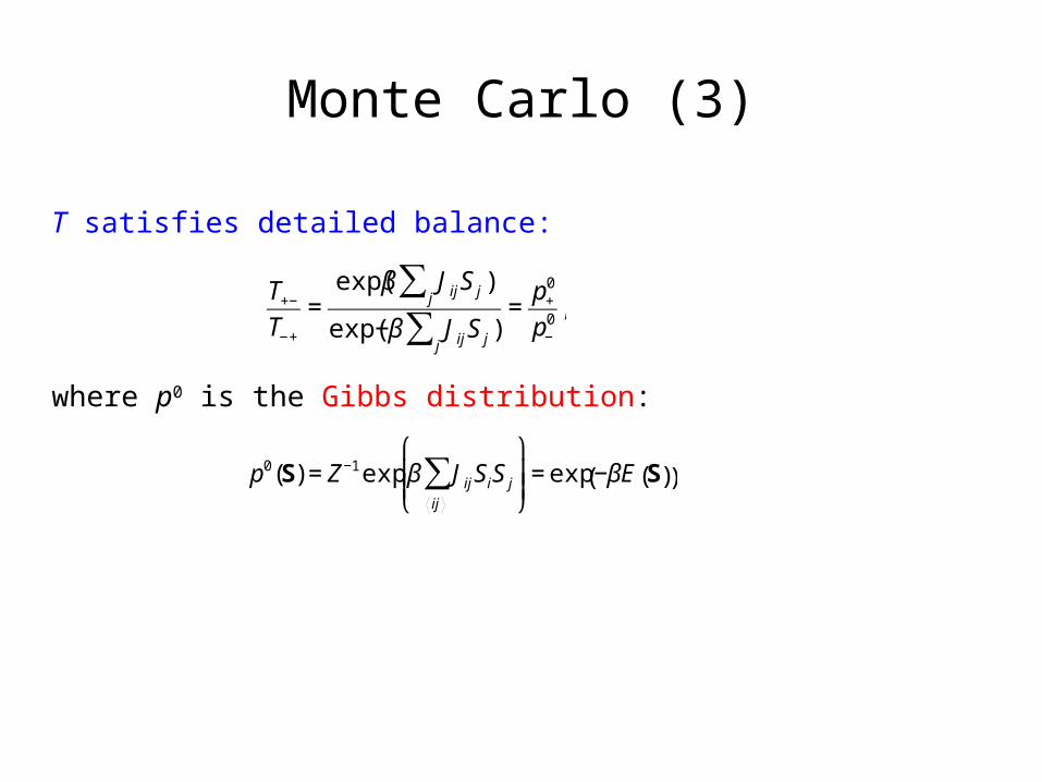
Monte Carlo (3)
T satisfies detailed balance:
where p0 is the Gibbs distribution:
€
T+−
T−+
=exp(β JijS jj
∑ )
exp(−β JijS jj∑ )
=p+
0
p−0,
€
p0(S) = Z−1 exp β JijSiS j
ij
∑ ⎛
⎝ ⎜ ⎜
⎞
⎠ ⎟ ⎟= exp −βE S( )( )
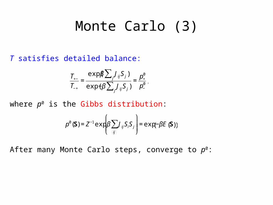
Monte Carlo (3)
T satisfies detailed balance:
where p0 is the Gibbs distribution:
After many Monte Carlo steps, converge to p0:
€
T+−
T−+
=exp(β JijS jj
∑ )
exp(−β JijS jj∑ )
=p+
0
p−0,
€
p0(S) = Z−1 exp β JijSiS j
ij
∑ ⎛
⎝ ⎜ ⎜
⎞
⎠ ⎟ ⎟= exp −βE S( )( )

Monte Carlo (3)
T satisfies detailed balance:
where p0 is the Gibbs distribution:
After many Monte Carlo steps, converge to p0: S’s sample Gibbs distribution
€
T+−
T−+
=exp(β JijS jj
∑ )
exp(−β JijS jj∑ )
=p+
0
p−0,
€
p0(S) = Z−1 exp β JijSiS j
ij
∑ ⎛
⎝ ⎜ ⎜
⎞
⎠ ⎟ ⎟= exp −βE S( )( )

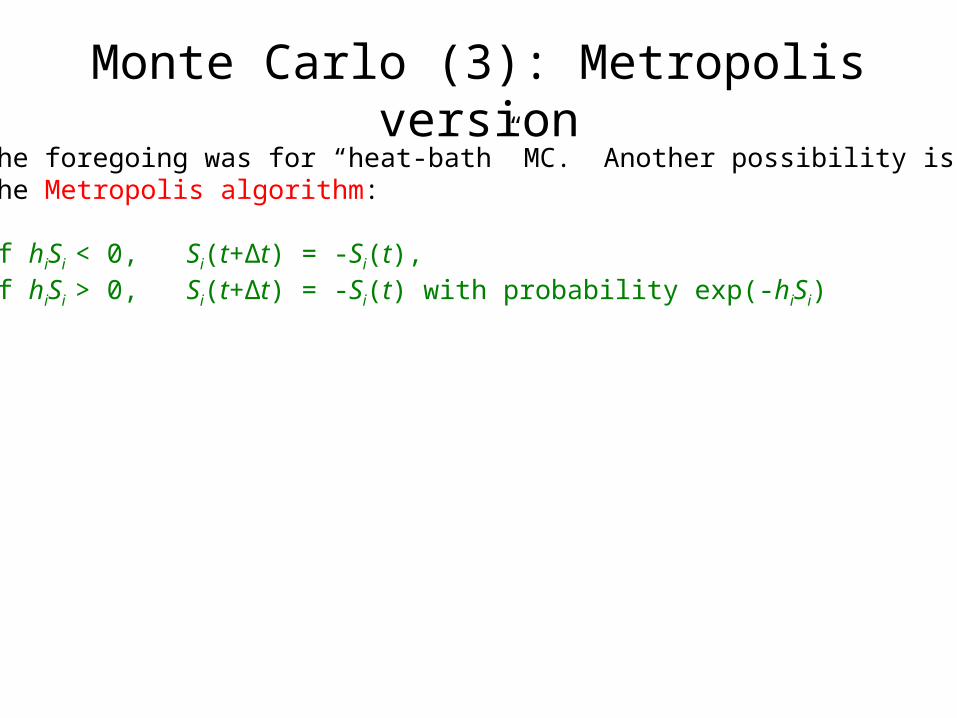
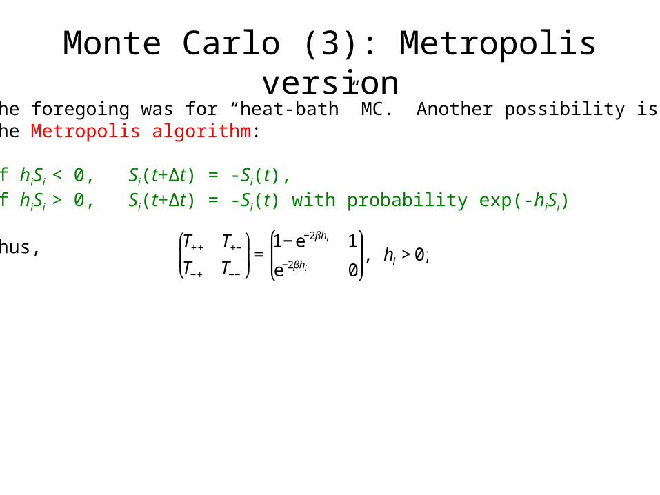
Monte Carlo (3): Metropolis versionThe foregoing was for “heat-bath” MC. Another possibility isthe Metropolis algorithm:

Monte Carlo (3): Metropolis versionThe foregoing was for “heat-bath” MC. Another possibility isthe Metropolis algorithm:
If hiSi < 0, Si(t+Δt) = -Si(t),
Monte Carlo (3): Metropolis versionThe foregoing was for “heat-bath” MC. Another possibility isthe Metropolis algorithm:
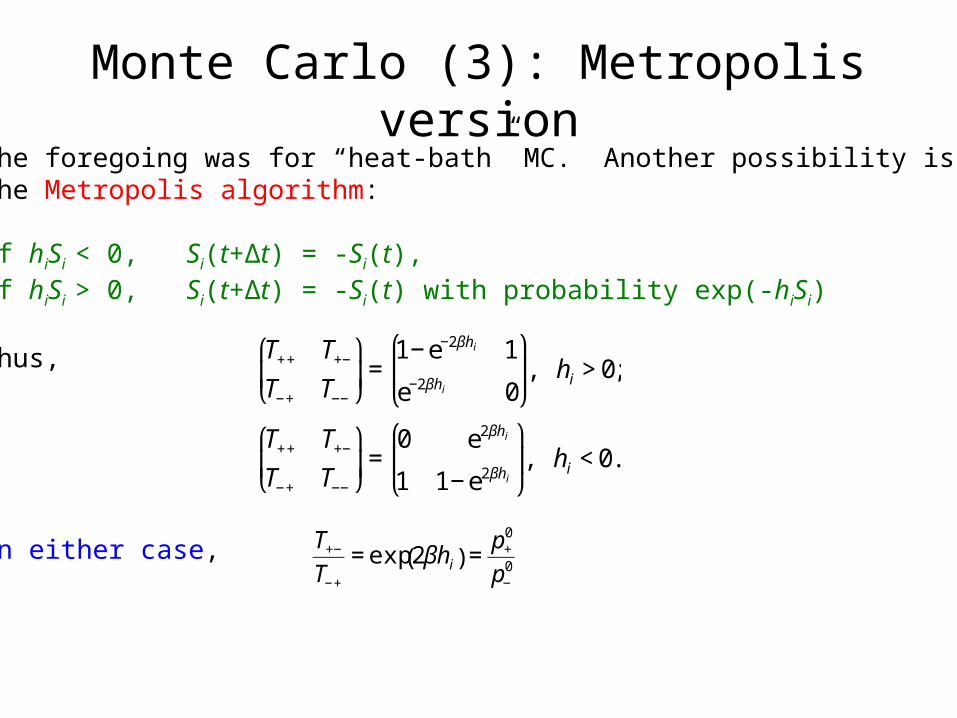
If hiSi < 0, Si(t+Δt) = -Si(t), If hiSi > 0, Si(t+Δt) = -Si(t) with probability exp(-hiSi)
Monte Carlo (3): Metropolis versionThe foregoing was for “heat-bath” MC. Another possibility isthe Metropolis algorithm:
If hiSi < 0, Si(t+Δt) = -Si(t), If hiSi > 0, Si(t+Δt) = -Si(t) with probability exp(-hiSi)
Thus,
€
T++ T+−
T−+ T−−
⎛
⎝ ⎜
⎞
⎠ ⎟=
1− e−2βhi 1
e−2βhi 0
⎛
⎝ ⎜
⎞
⎠ ⎟, hi > 0;

Monte Carlo (3): Metropolis versionThe foregoing was for “heat-bath” MC. Another possibility isthe Metropolis algorithm:
If hiSi < 0, Si(t+Δt) = -Si(t), If hiSi > 0, Si(t+Δt) = -Si(t) with probability exp(-hiSi)
Thus,
€
T++ T+−
T−+ T−−
⎛
⎝ ⎜
⎞
⎠ ⎟=
1− e−2βhi 1
e−2βhi 0
⎛
⎝ ⎜
⎞
⎠ ⎟, hi > 0;
T++ T+−
T−+ T−−
⎛
⎝ ⎜
⎞
⎠ ⎟=
0 e2βhi
1 1− e2βhi
⎛
⎝ ⎜
⎞
⎠ ⎟, hi < 0.
Monte Carlo (3): Metropolis versionThe foregoing was for “heat-bath” MC. Another possibility isthe Metropolis algorithm:
If hiSi < 0, Si(t+Δt) = -Si(t), If hiSi > 0, Si(t+Δt) = -Si(t) with probability exp(-hiSi)
Thus,
In either case,
€
T++ T+−
T−+ T−−
⎛
⎝ ⎜
⎞
⎠ ⎟=
1− e−2βhi 1
e−2βhi 0
⎛
⎝ ⎜
⎞
⎠ ⎟, hi > 0;
T++ T+−
T−+ T−−
⎛
⎝ ⎜
⎞
⎠ ⎟=
0 e2βhi
1 1− e2βhi
⎛
⎝ ⎜
⎞
⎠ ⎟, hi < 0.
€
T+−
T−+
= exp 2βhi( ) =p+
0
p−0

Monte Carlo (3): Metropolis versionThe foregoing was for “heat-bath” MC. Another possibility isthe Metropolis algorithm:
If hiSi < 0, Si(t+Δt) = -Si(t), If hiSi > 0, Si(t+Δt) = -Si(t) with probability exp(-hiSi)
Thus,
In either case,
i.e., detailed balance with Gibbs
€
T++ T+−
T−+ T−−
⎛
⎝ ⎜
⎞
⎠ ⎟=
1− e−2βhi 1
e−2βhi 0
⎛
⎝ ⎜
⎞
⎠ ⎟, hi > 0;
T++ T+−
T−+ T−−
⎛
⎝ ⎜
⎞
⎠ ⎟=
0 e2βhi
1 1− e2βhi
⎛
⎝ ⎜
⎞
⎠ ⎟, hi < 0.
€
T+−
T−+
= exp 2βhi( ) =p+
0
p−0
€
p+−0
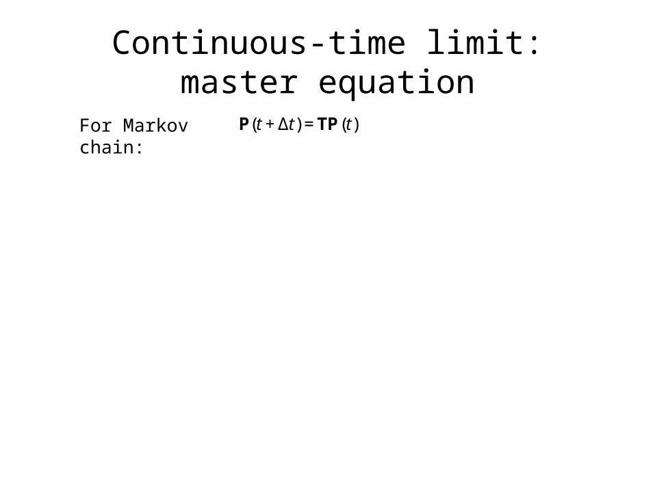
Continuous-time limit:master equation
€
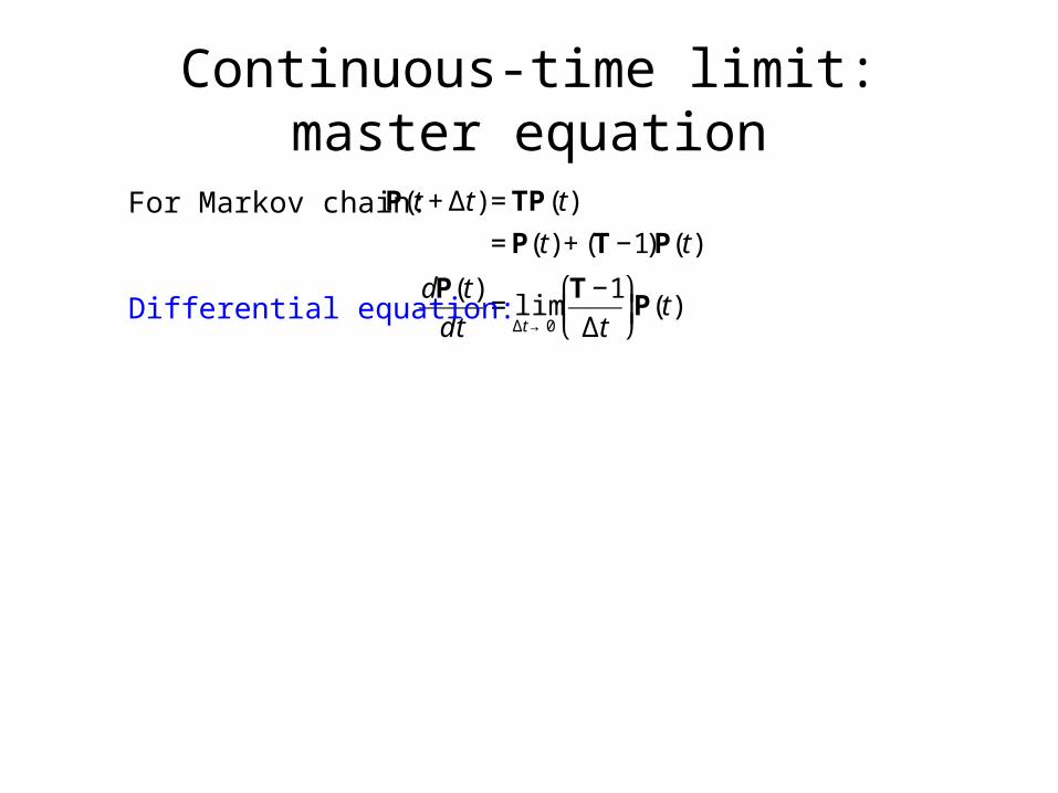
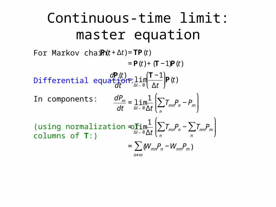
P(t + Δt) =TP(t)For Markov chain:

Continuous-time limit:master equation
€
P(t + Δt) =TP(t)
= P(t) + (T−1)P(t)
For Markov chain:
Continuous-time limit:master equation
€
P(t + Δt) =TP(t)
= P(t) + (T−1)P(t)
dP(t)
dt= lim
Δt →0
T−1
Δt
⎛
⎝ ⎜
⎞
⎠ ⎟P(t)
For Markov chain:
Differential equation:

Continuous-time limit:master equation
€
P(t + Δt) =TP(t)
= P(t) + (T−1)P(t)
dP(t)
dt= lim
Δt →0
T−1
Δt
⎛
⎝ ⎜
⎞
⎠ ⎟P(t)
dPm
dt= lim
Δt →0
1
ΔtTmnPn − Pm
n
∑ ⎛
⎝ ⎜
⎞
⎠ ⎟
For Markov chain:
Differential equation:
In components:
Continuous-time limit:master equation
€
P(t + Δt) =TP(t)
= P(t) + (T−1)P(t)
dP(t)
dt= lim
Δt →0
T−1
Δt
⎛
⎝ ⎜
⎞
⎠ ⎟P(t)
dPm
dt= lim
Δt →0
1
ΔtTmnPn − Pm
n
∑ ⎛
⎝ ⎜
⎞
⎠ ⎟
= limΔt →0
1
ΔtTmnPn − Tnm
n
∑ Pm
n
∑ ⎛
⎝ ⎜
⎞
⎠ ⎟
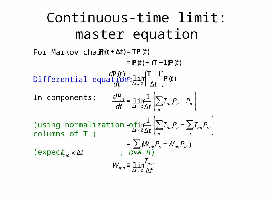
= WmnPn −WnmPm( )n≠m
∑
For Markov chain:
Differential equation:
In components:
(using normalization ofcolumns of T:)
Continuous-time limit:master equation
€
P(t + Δt) =TP(t)
= P(t) + (T−1)P(t)
dP(t)
dt= lim
Δt →0
T−1
Δt
⎛
⎝ ⎜
⎞
⎠ ⎟P(t)
dPm
dt= lim
Δt →0
1
ΔtTmnPn − Pm
n
∑ ⎛
⎝ ⎜
⎞
⎠ ⎟
= limΔt →0
1
ΔtTmnPn − Tnm
n
∑ Pm
n
∑ ⎛
⎝ ⎜
⎞
⎠ ⎟
= WmnPn −WnmPm( )n≠m
∑
Wmn ≡ limΔt →0
Tmn
Δt
For Markov chain:
Differential equation:
In components:
(using normalization ofcolumns of T:)
(expect , m ≠ n)
€
Tmn ∝Δt
transition rate matrix