Embed Size (px)
Citation preview
2E5295/5B5749 Convex optimization with engineering applications
Lecture 3
Linear programming and the simplex method
A. Forsgren, KTH 1 Lecture 3 Convex optimization 2006/2007
Optimality conditions
For f differentiable, consider
(P )minimize f(x)
subject to x ∈ S ⊆ IRn.
Proposition. Assume that S is a convex subset of IRn, and assume
that f : S → IR is a convex differentiable function on S. Then, x∗ ∈ S
is a global minimizer to (P ) if and only if ∇f(x∗)T(x− x∗) ≥ 0 for all
x ∈ S.
This condition is not immediate to verify, since it involves all feasible x.
We will consider more immediate conditions.
A. Forsgren, KTH 2 Lecture 3 Convex optimization 2006/2007
Linear program
A linear program is a convex optimization problem on the form
(LP )
minimizex∈IRn
cTx
subject to Ax = b,
x ≥ 0.
May be written on many (equivalent) forms.
The feasible set is a polyhedron, i.e., given by the intersection of a finite
number of hyperplanes in IRn.
A. Forsgren, KTH 3 Lecture 3 Convex optimization 2006/2007
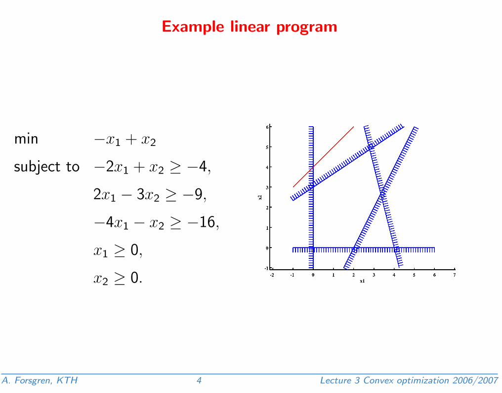
Example linear program
min −x1 + x2
subject to −2x1 + x2 ≥ −4,
2x1 − 3x2 ≥ −9,
−4x1 − x2 ≥ −16,
x1 ≥ 0,
x2 ≥ 0.
A. Forsgren, KTH 4 Lecture 3 Convex optimization 2006/2007
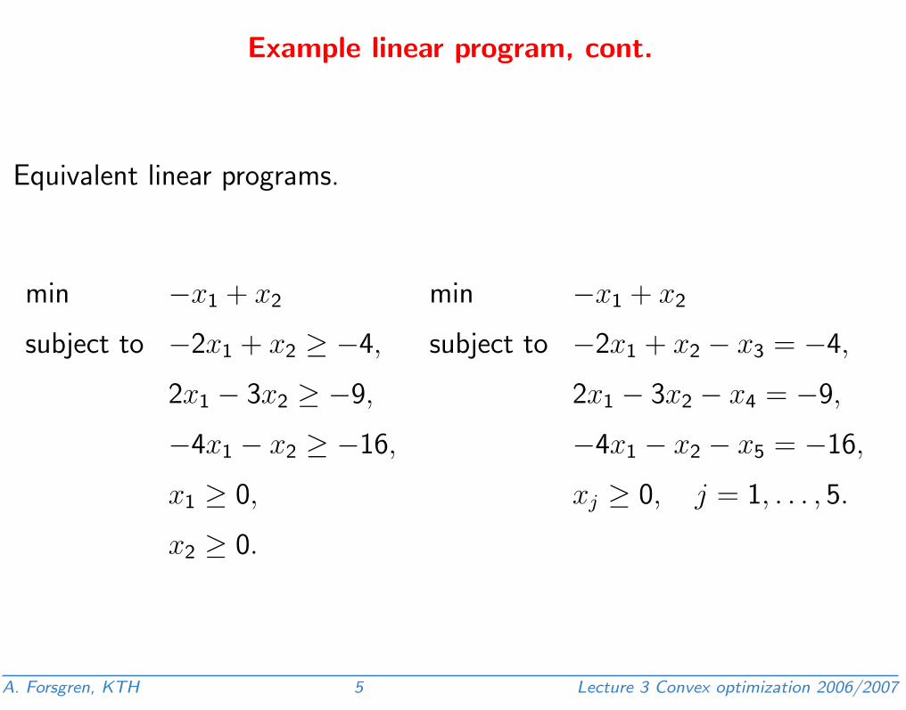
Example linear program, cont.
Equivalent linear programs.
min −x1 + x2
subject to −2x1 + x2 ≥ −4,
2x1 − 3x2 ≥ −9,
−4x1 − x2 ≥ −16,
x1 ≥ 0,
x2 ≥ 0.
min −x1 + x2
subject to −2x1 + x2 − x3 = −4,
2x1 − 3x2 − x4 = −9,
−4x1 − x2 − x5 = −16,
xj ≥ 0, j = 1, . . . , 5.
A. Forsgren, KTH 5 Lecture 3 Convex optimization 2006/2007
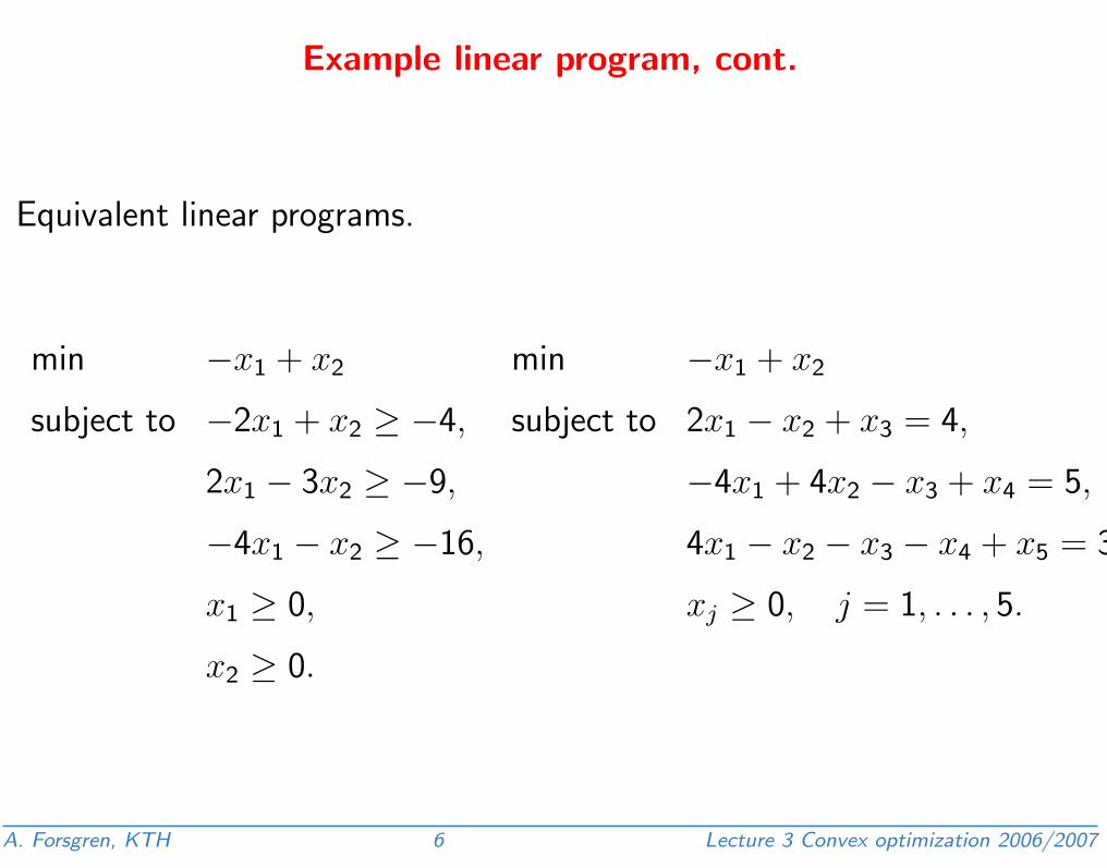
Example linear program, cont.
Equivalent linear programs.
min −x1 + x2
subject to −2x1 + x2 ≥ −4,
2x1 − 3x2 ≥ −9,
−4x1 − x2 ≥ −16,
x1 ≥ 0,
x2 ≥ 0.
min −x1 + x2
subject to 2x1 − x2 + x3 = 4,
−4x1 + 4x2 − x3 + x4 = 5,
4x1 − x2 − x3 − x4 + x5 = 3,
xj ≥ 0, j = 1, . . . , 5.
A. Forsgren, KTH 6 Lecture 3 Convex optimization 2006/2007
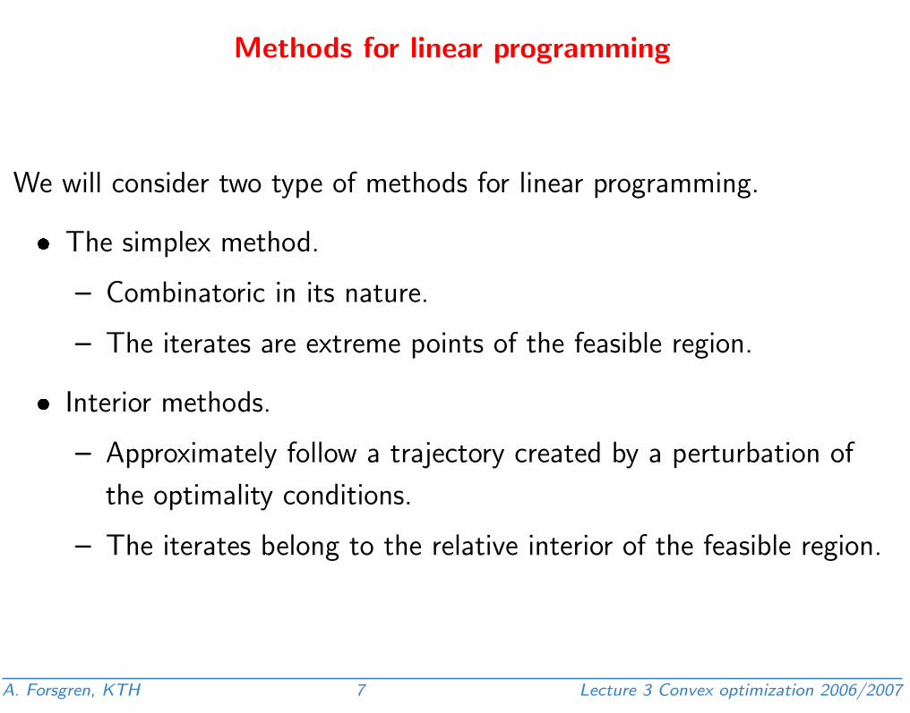
Methods for linear programming
We will consider two type of methods for linear programming.
� The simplex method.
– Combinatoric in its nature.
– The iterates are extreme points of the feasible region.
� Interior methods.
– Approximately follow a trajectory created by a perturbation of
the optimality conditions.
– The iterates belong to the relative interior of the feasible region.
A. Forsgren, KTH 7 Lecture 3 Convex optimization 2006/2007
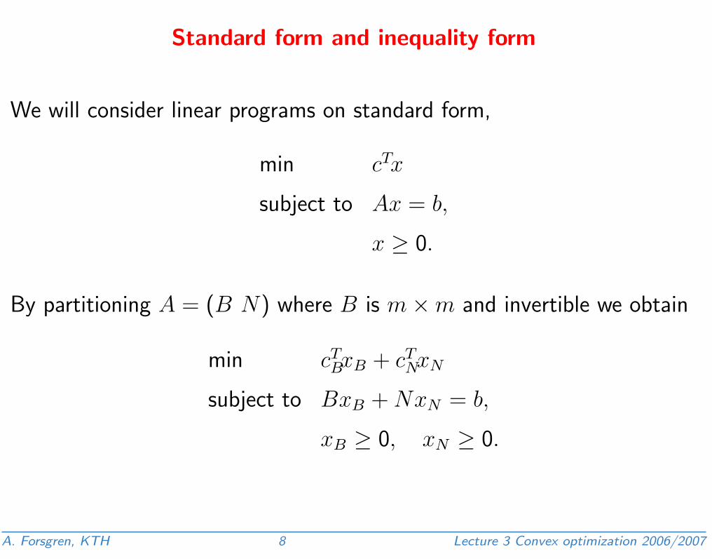
Standard form and inequality form
We will consider linear programs on standard form,
min cTx
subject to Ax = b,
x ≥ 0.
By partitioning A = (B N) where B is m×m and invertible we obtain
min cTBxB + cT
NxN
subject to BxB + NxN = b,
xB ≥ 0, xN ≥ 0.
A. Forsgren, KTH 8 Lecture 3 Convex optimization 2006/2007
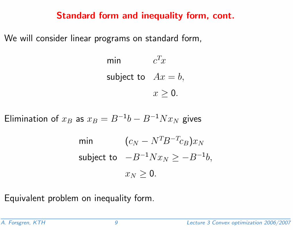
Standard form and inequality form, cont.
We will consider linear programs on standard form,
min cTx
subject to Ax = b,
x ≥ 0.
Elimination of xB as xB = B−1b−B−1NxN gives
min (cN −NTB−TcB)xN
subject to −B−1NxN ≥ −B−1b,
xN ≥ 0.
Equivalent problem on inequality form.
A. Forsgren, KTH 9 Lecture 3 Convex optimization 2006/2007
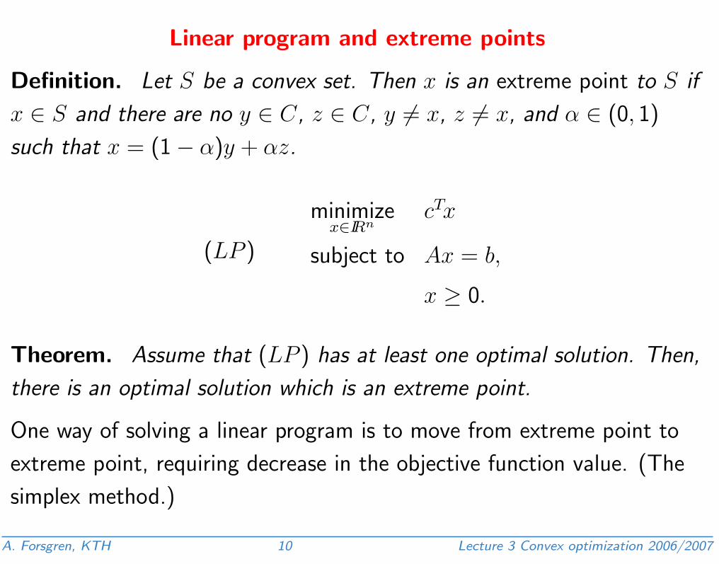
Linear program and extreme points
Definition. Let S be a convex set. Then x is an extreme point to S if
x ∈ S and there are no y ∈ C, z ∈ C, y 6= x, z 6= x, and α ∈ (0, 1)
such that x = (1− α)y + αz.
(LP )
minimizex∈IRn
cTx
subject to Ax = b,
x ≥ 0.
Theorem. Assume that (LP ) has at least one optimal solution. Then,
there is an optimal solution which is an extreme point.
One way of solving a linear program is to move from extreme point to
extreme point, requiring decrease in the objective function value. (The
simplex method.)
A. Forsgren, KTH 10 Lecture 3 Convex optimization 2006/2007
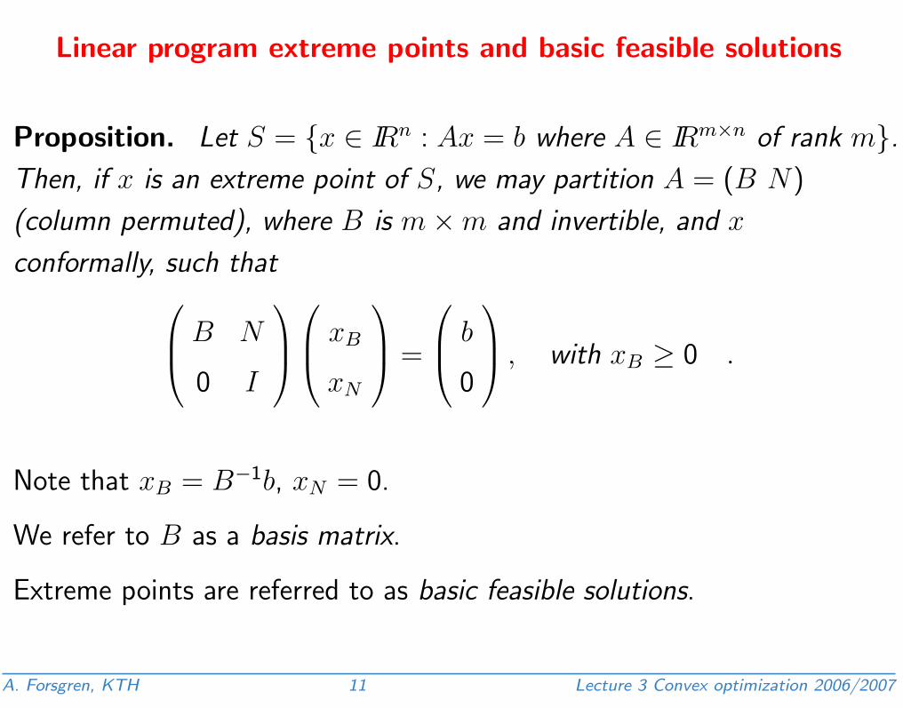
Linear program extreme points and basic feasible solutions
Proposition. Let S = {x ∈ IRn : Ax = b where A ∈ IRm×n of rank m}.Then, if x is an extreme point of S, we may partition A = (B N)
(column permuted), where B is m×m and invertible, and x
conformally, such that B N
0 I
xB
xN
=
b
0
, with xB ≥ 0 .
Note that xB = B−1b, xN = 0.
We refer to B as a basis matrix.
Extreme points are referred to as basic feasible solutions.
A. Forsgren, KTH 11 Lecture 3 Convex optimization 2006/2007

Optimality of basic feasible solution
Assume that we have a basic feasible solution B N
0 I
xB
xN
=
b
0
.
Proposition. The basic feasible solution is optimal if cTpi ≥ 0,
i = 1, . . . , n−m, where pi is given by B N
0 I
pi
B
piN
=
0
ei
, i = 1, . . . , n−m.
Proof. If x̃ is feasible, it must hold that x̃− x =∑n−m
i=1 γipi, where
γi ≥ 0, i = 1, . . . , n−m. Hence, cT(x̃− x) ≥ 0.
A. Forsgren, KTH 12 Lecture 3 Convex optimization 2006/2007
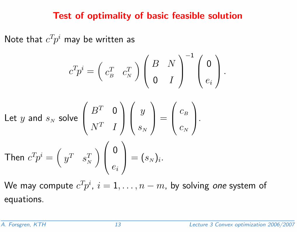
Test of optimality of basic feasible solution
Note that cTpi may be written as
cTpi =(
cTB cT
N
) B N
0 I
−1 0
ei
.
Let y and sN solve
BT 0
NT I
y
sN
=
cB
cN
.
Then cTpi =(
yT sTN
) 0
ei
= (sN)i.
We may compute cTpi, i = 1, . . . , n−m, by solving one system of
equations.
A. Forsgren, KTH 13 Lecture 3 Convex optimization 2006/2007
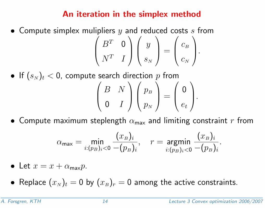
An iteration in the simplex method
� Compute simplex mulipliers y and reduced costs s from BT 0
NT I
y
sN
=
cB
cN
.
� If (sN)t < 0, compute search direction p from B N
0 I
pB
pN
=
0
et
.
� Compute maximum steplength αmax and limiting constraint r from
αmax = mini:(pB)i<0
(xB)i
−(pB)i
, r = argmini:(pB)i<0
(xB)i
−(pB)i
.
� Let x = x + αmaxp.
� Replace (xN)t = 0 by (xB)r = 0 among the active constraints.
A. Forsgren, KTH 14 Lecture 3 Convex optimization 2006/2007
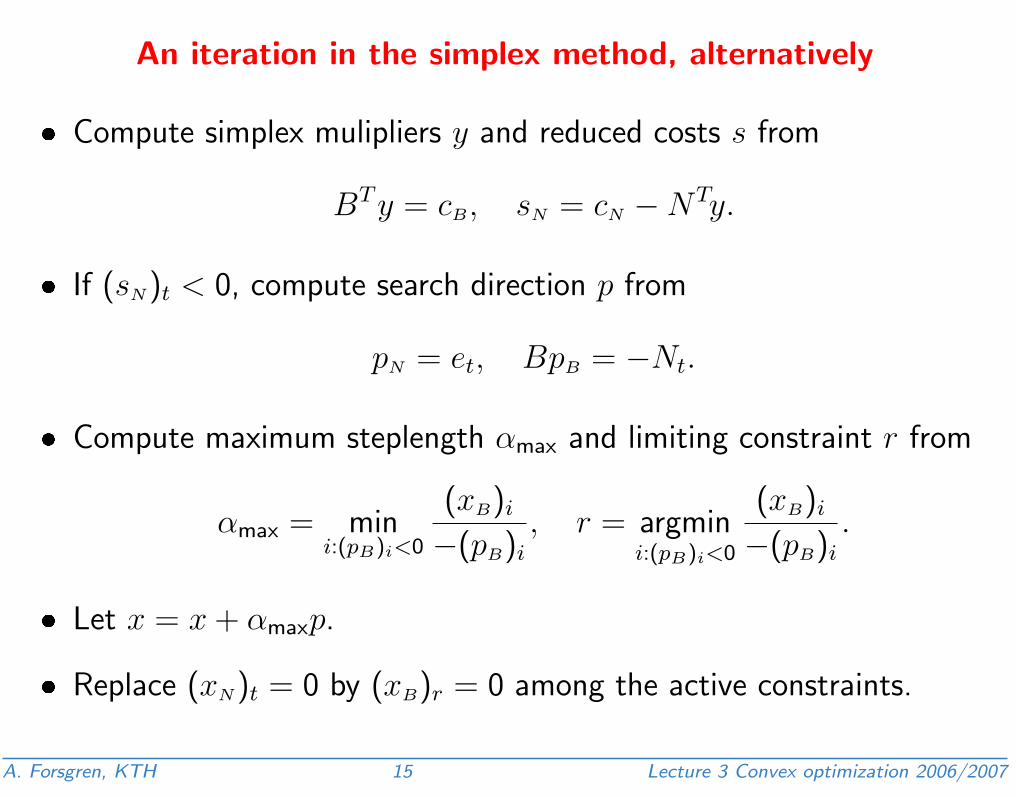
An iteration in the simplex method, alternatively
� Compute simplex mulipliers y and reduced costs s from
BT y = cB, sN = cN −NTy.
� If (sN)t < 0, compute search direction p from
pN = et, BpB = −Nt.
� Compute maximum steplength αmax and limiting constraint r from
αmax = mini:(pB)i<0
(xB)i
−(pB)i
, r = argmini:(pB)i<0
(xB)i
−(pB)i
.
� Let x = x + αmaxp.
� Replace (xN)t = 0 by (xB)r = 0 among the active constraints.
A. Forsgren, KTH 15 Lecture 3 Convex optimization 2006/2007
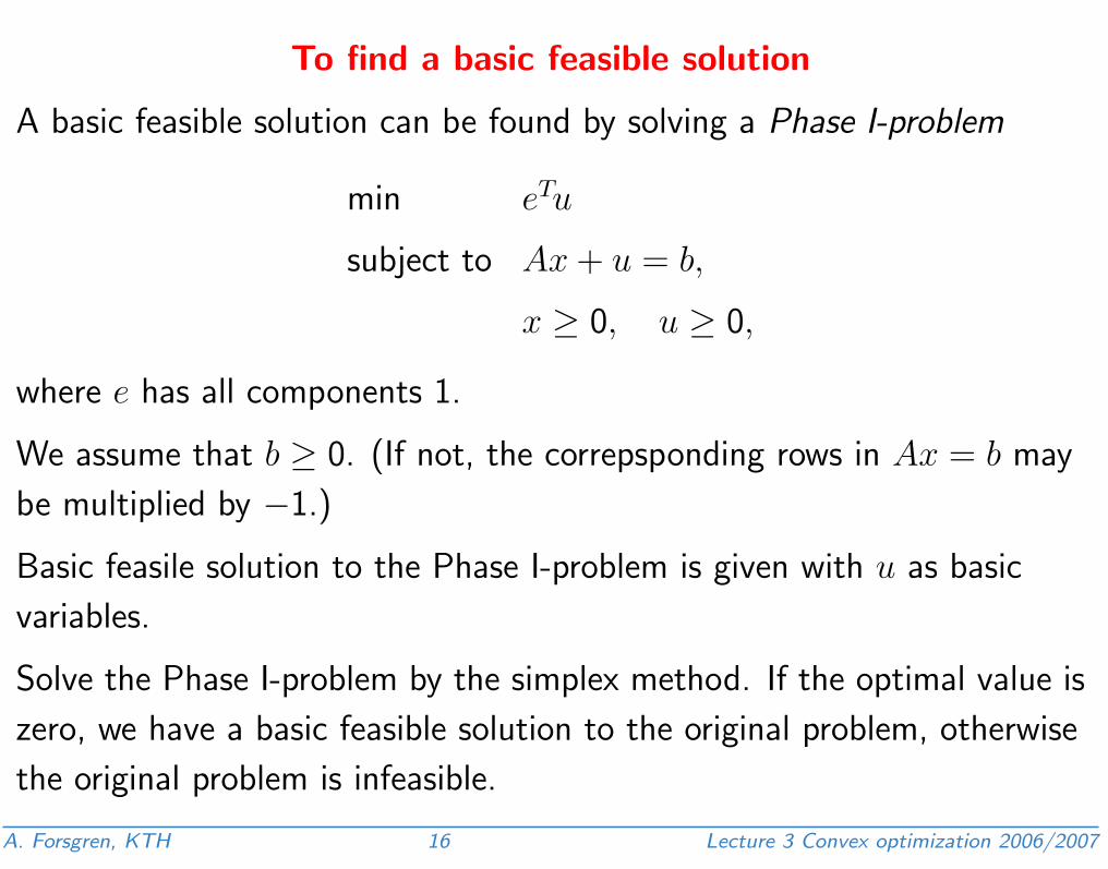
To find a basic feasible solution
A basic feasible solution can be found by solving a Phase I-problem
min eTu
subject to Ax + u = b,
x ≥ 0, u ≥ 0,
where e has all components 1.
We assume that b ≥ 0. (If not, the correpsponding rows in Ax = b may
be multiplied by −1.)
Basic feasile solution to the Phase I-problem is given with u as basic
variables.
Solve the Phase I-problem by the simplex method. If the optimal value is
zero, we have a basic feasible solution to the original problem, otherwise
the original problem is infeasible.
A. Forsgren, KTH 16 Lecture 3 Convex optimization 2006/2007
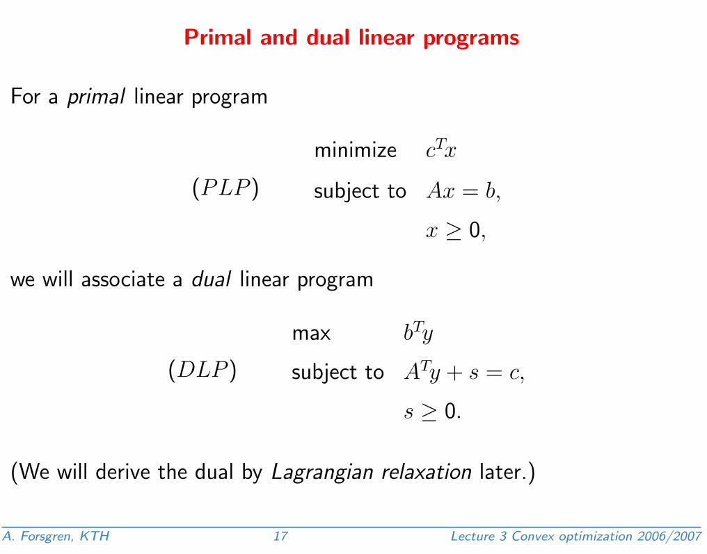
Primal and dual linear programs
For a primal linear program
(PLP )
minimize cTx
subject to Ax = b,
x ≥ 0,
we will associate a dual linear program
(DLP )
max bTy
subject to ATy + s = c,
s ≥ 0.
(We will derive the dual by Lagrangian relaxation later.)
A. Forsgren, KTH 17 Lecture 3 Convex optimization 2006/2007
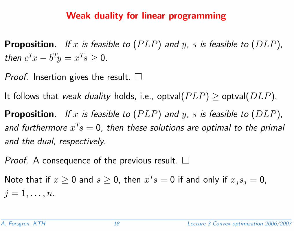
Weak duality for linear programming
Proposition. If x is feasible to (PLP ) and y, s is feasible to (DLP ),
then cTx− bTy = xTs ≥ 0.
Proof. Insertion gives the result.
It follows that weak duality holds, i.e., optval(PLP ) ≥ optval(DLP ).
Proposition. If x is feasible to (PLP ) and y, s is feasible to (DLP ),
and furthermore xTs = 0, then these solutions are optimal to the primal
and the dual, respectively.
Proof. A consequence of the previous result.
Note that if x ≥ 0 and s ≥ 0, then xTs = 0 if and only if xjsj = 0,
j = 1, . . . , n.
A. Forsgren, KTH 18 Lecture 3 Convex optimization 2006/2007
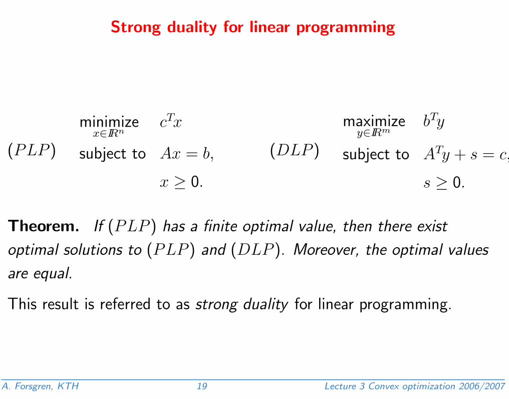
Strong duality for linear programming
(PLP )
minimizex∈IRn
cTx
subject to Ax = b,
x ≥ 0.
(DLP )
maximizey∈IRm
bTy
subject to ATy + s = c,
s ≥ 0.
Theorem. If (PLP ) has a finite optimal value, then there exist
optimal solutions to (PLP ) and (DLP ). Moreover, the optimal values
are equal.
This result is referred to as strong duality for linear programming.
A. Forsgren, KTH 19 Lecture 3 Convex optimization 2006/2007


![A KKT Simplex Method for Efficiently Solving Linear ...mcruz/paper27.pdf · paper is an example [11, 23]. In this kind of problems, the analytic center of the polyhedron of feasible](https://img.pdfslide.us/doc/110x75/5f0353ea7e708231d408ab27/a-kkt-simplex-method-for-efficiently-solving-linear-mcruzpaper27pdf-paper.jpg)


![1.2. Simplex Methodwebpages.iust.ac.ir/yaghini/Courses/RTP_882/LP_Review_02.pdfwith basis B = [a1, a2, a5] is given by Simplex Method All three of the foregoing basic feasible solutions](https://img.pdfslide.us/doc/110x75/5fdfd97dfed59060fc64780c/12-simplex-with-basis-b-a1-a2-a5-is-given-by-simplex-method-all-three-of.jpg)