Embed Size (px)
Citation preview

7/21/2017
1
Lecture 28 Slide 1
EE 5337
Computational Electromagnetics (CEM)
Lecture #28
Method of Momentsfor Thin Wire Antennas These notes may contain copyrighted material obtained under fair use rules. Distribution of these materials is strictly prohibited
InstructorDr. Raymond Rumpf(915) 747‐[email protected]
Outline
• Introduction
• Pocklington’s and Hallen’s Integral Equations
• Method of Moments Solution to Pocklington’s Equation
• Thin Wire Excitations
• Impedance Loading
Lecture 28 Slide 2

7/21/2017
2
Lecture 28 Slide 3
Introduction
Lecture 28 Slide 4
The Method of Moments
Lf g
, ,n m n mn
a v Lv v g
1 11 1 1 2
1 22 1 2 2
,, ,
,, ,
,N N
a
a
a
v Lgv Lv v Lv
v Lgv Lv v Lv
v Lg
n nn
a Lv gn nn
af v Galerkin Method Integral Equation
•Usually uses PEC approximation•Usually based on current
2
22inc 2
2 4L
jkrL
z z
j eE I z k dz
z r
• Converts a linear equation to a matrix equation
The Method of Moments
11 12 13 14 15 16 17 1
21 22 23 24 25 26 27 2
31 32 33 34 35 36 37 3
41 42 43 44 45 46 47 4
51 52 53 54 55 56 57 5
61 62 63 64 65 66 67 6
71 72 73 74 75 76 77 7
z z z z z z z i
z z z z z z z i
z z z z z z z i
z z z z z z z i
z z z z z z z i
z z z z z z z i
z z z z z z z i
1
2
3
4
5
6
7
v
v
v
v
v
v
v
1i2i
3i4i
5i6i
7i1v
2v3v
4v5v
6v7v
7/21/2017
3
Lecture 28 Slide 5
Pocklington’s and Hallen’sIntegral Equations
Lecture 28 Slide 6
Maxwell’s Equations
Maxwell’s equations in the frequency‐domain can be written as
0
0
E j H
H J j E
E
H
• Frequency‐domain•Differential form• Constitutive relations have be substituted

7/21/2017
4
Lecture 28 Slide 7
Definition of Magnetic Vector Potential
Since , the term is solenoidal. This means it only forms loops so it can be written in terms of the curl of some other vector function .
H A
0H
H
We call that other vector function the magnetic vector potential because it shares many attributes of the electric scalar potential.
The magnetic vector potential is not a physical quantity, but is useful in simplifying the mathematics of some electromagnetic analyses.
A
A
Lecture 28 Slide 8
Definition of Electric Scalar Potential
We can substitute the magnetic vector potential into to arrive at
E j H
The term inside the parentheses has zero curl. This means it is “conservative” and behaves like a static electric field. We define the electric scalar potential from this quantity.
E j A
0
0
AE j
E j A
E j A

7/21/2017
5
Lecture 28 Slide 9
Lorentz Gauge Condition
We now have more variables than we have degrees of freedom so we need to “fix the gauge.” We do this be relating some of the variables.
We have yet to specify anything about the divergence of the magnetic vector potential. For convenience and to fix the gauge, we let
A j
Lecture 28 Slide 10
Wave Equation in Terms of Potentials (1 of 2)
First, we write in terms of the magnetic vector potential.
AJ j E
H J j E
To simplify this further, we must assume our antenna is embedded in a homogeneous medium. Now our equation reduces to
2A A J j E
We now substitute the electric scalar potential into this equation.
2 2A A j A J
7/21/2017
6
Lecture 28 Slide 11
Wave Equation in Terms of Potentials (2 of 2)
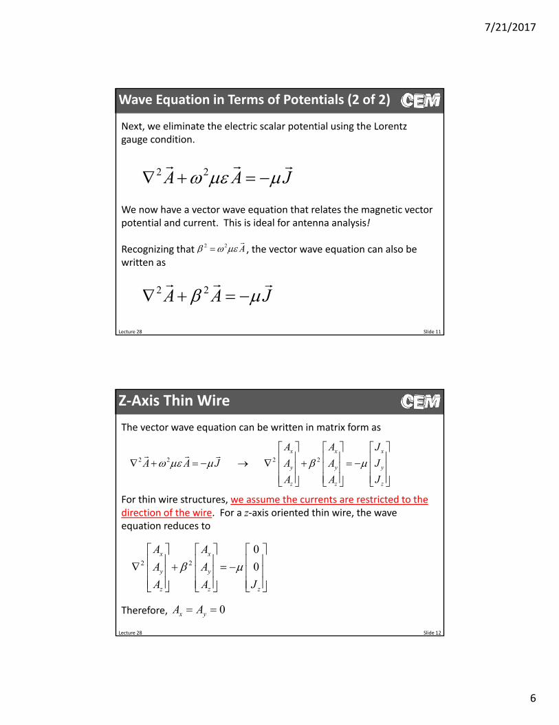
Next, we eliminate the electric scalar potential using the Lorentz gauge condition.
2 2A A J
We now have a vector wave equation that relates the magnetic vector potential and current. This is ideal for antenna analysis!
Recognizing that , the vector wave equation can also be written as
2 2A A J
2 2 A
Lecture 28 Slide 12
Z‐Axis Thin Wire
The vector wave equation can be written in matrix form as
2 2 2 2 x x x
y y y
z z z
A A J
A A J A A J
A A J
For thin wire structures, we assume the currents are restricted to the direction of the wire. For a z‐axis oriented thin wire, the wave equation reduces to
2 2
0
0x x
y y
z z z
A A
A A
A A J
Therefore, 0x yA A

7/21/2017
7
Lecture 28 Slide 13
Revised Equations
Given the z‐axis thin wire approximation, the Lorentz gauge condition reduces to
zAA j jz
Our definition of electric scalar potential reduces to
z zE j A E j Az
Combining the above equations, we arrive at
22
2
1 zz z
AE A
j z
This is not our differential equation to solve. This is how we will calculate the electric field from the magnetic vector potential.
Lecture 28 Slide 14
What is a Green’s Function
Suppose a device can be decomposed into many identical small elements.
If the response of one of these elements can be obtained, then the overall solution is the superposition of the response of all of the tiny elements comprising the device.
The response of one of these tiny elements is called the Green’s function. The overall solution is obtained by integrating the Green’s function over the domain of the device.

7/21/2017
8
Lecture 28 Slide 15
Illustration of a Green’s Function
We can visualizing integrating a Green’s function this way…
+ + + =
Observation point
Lecture 28 Slide 16
Green’s Function for Small Current Element (1 of 2)
Our wave equation for the z‐axis thin wire is
2 2z z zA A J
Away from the wire, Jz= 0 and the differential equation reduces to
2 2 0
This has a solution of
, 4
j ReG r r R r r
R
observation point
location of point source of current
r
r
observation pointr
point along wirer
R
7/21/2017
9
Lecture 28 Slide 17
Green’s Function for Small Current Element (2 of 2)
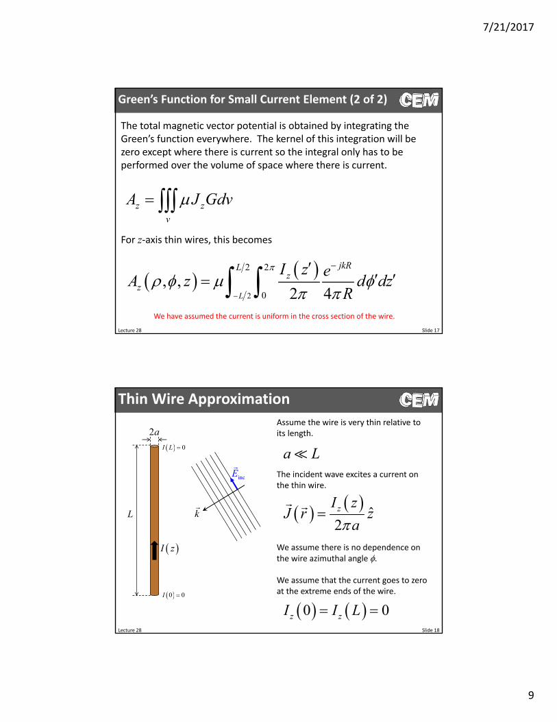
The total magnetic vector potential is obtained by integrating the Green’s function everywhere. The kernel of this integration will be zero except where there is current so the integral only has to be performed over the volume of space where there is current.
z z
v
A J Gdv For z‐axis thin wires, this becomes
2
2 2
0, ,
2 4L
jkRLz
z
I z eA z d dz
R
We have assumed the current is uniform in the cross section of the wire.
Lecture 28 Slide 18
Thin Wire Approximation
L
2a
I z
k
Assume the wire is very thin relative to its length.
The incident wave excites a current on the thin wire.
a LincE
ˆ
2zI z
J r za
We assume there is no dependence on the wire azimuthal angle .
We assume that the current goes to zero at the extreme ends of the wire. 0 0I
0I L
0 0z zI I L

7/21/2017
10
Lecture 28 Slide 19
Magnetic Vector Potential (1 of 3)
The magnetic vector potential on the surface of the wire due to the current in the wire is written in terms of a surface integral.
2
2 2
0, ,
2 4L
jkRLz
z
I z eA z d dz
R
Where R is the distance from the point in the integral to the observation point.
2 2R z z
Since the magnetic vector potential is written on the surface of the wire, ’=a.
2 2 2 2 cosa a Due to the cylindrical symmetry, we can replace ’‐with just ’ without loss of generality.
2 2 2 2 cosr r We integrate on surface of cylinder
Lecture 28 Slide 20
Magnetic Vector Potential (2 of 3)
The magnetic vector potential can now be written as
2
2 2
0
2 2 2
, ,2 4
2 cos
L
jkRLz
z
I z eA z d dz
R
R z z a a
If a is very small,
2 2R z z
Then there is no dependence and the magnetic vector potential equation reduces to
2
2
,4L
jkRL
z z
eA z I z dz
R
“Thin wire approximation with reduced kernel”
The surface integral has been reduced to a line integral.
7/21/2017
11
Lecture 28 Slide 21
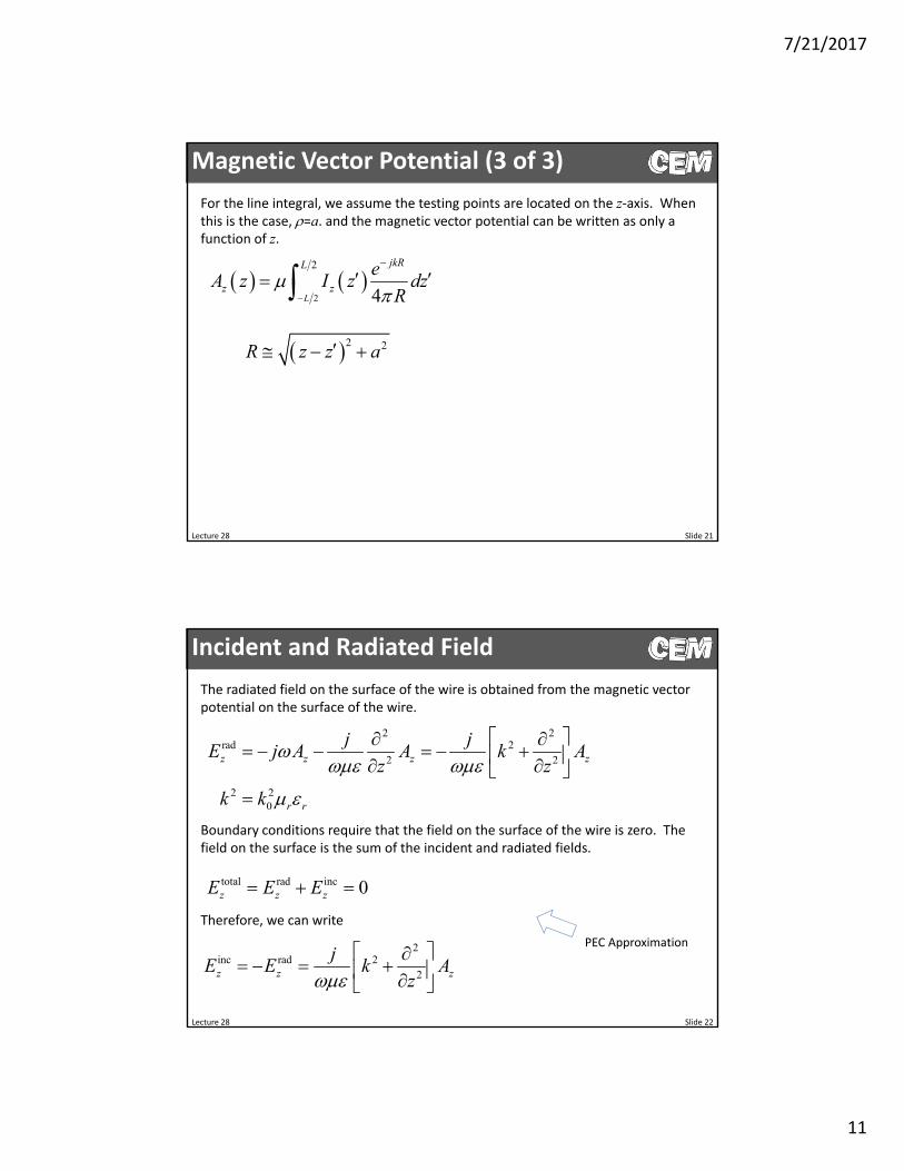
Magnetic Vector Potential (3 of 3)
For the line integral, we assume the testing points are located on the z‐axis. When this is the case, =a. and the magnetic vector potential can be written as only a function of z.
2 2R z z a
2
2
4L
jkRL
z z
eA z I z dz
R
Lecture 28 Slide 22
Incident and Radiated Field
The radiated field on the surface of the wire is obtained from the magnetic vector potential on the surface of the wire.
2 2rad 2
2 2
2 20
z z z z
r r
j jE j A A k A
z z
k k
total rad inc 0z z zE E E
Boundary conditions require that the field on the surface of the wire is zero. The field on the surface is the sum of the incident and radiated fields.
Therefore, we can write
2inc rad 2
2z z z
jE E k A
z
PEC Approximation

7/21/2017
12
Lecture 28 Slide 23
Hallen’s Integral Equation
Recall the following equations:
2
2
2inc 2
2
4L
jkRL
z z
z z
eA z I z dz
R
jE k A
z
Substituting the first equation into the second leads to Hallen’s integral equation.
2
2 2inc 2
2 4L
jkRL
z z
j eE z k I z dz
z R
2 2R z z a
Lecture 28 Slide 24
Pocklington’s Integral Equation
Starting with Hallen’s integral equation
We move the differential operator under the integral sign.
2
22inc 2
2 4L
jkRL
z z
j eE z I z k dz
z R
2
2 2inc 2
2 4L
jkRL
z z
j eE z k I z dz
z R
While Pocklington’s equation is the most famous and easier to solve, it is not as well behaved as Hallen’s equation resulting in slower convergence and poorer accuracy.

7/21/2017
13
Lecture 28 Slide 25
Visualizing Pocklington’s Integral Equation
2
22inc 2
2 4L
jkrL
z z
j eE z I z k dz
z r
We formulated Pocklington’sintegral equation with being a receiving antenna in mind.
We will implement the equation as a transmitting antenna.
k
incE
incE
Lecture 28 Slide 26
Convergence Comparison
L
2a
0
0
0.477
0.001
1
1r
r
L
a
70.3 inZ

7/21/2017
14
Lecture 28 Slide 27
Method of Moments Solution to
Pocklington’s Equation
Lecture 28 Slide 28
Setup for the Galerkin Method
This has the form of where
2
222 inc
2 4L
jkRL
z z
eI z k dz j E z
z R
We start with Pocklington’s integral equation in the following form.
L f g
2
222
2
inc
1L
4L
jkRL
z
z
ef I z k dz
j z R
f I z
g E z
7/21/2017
15
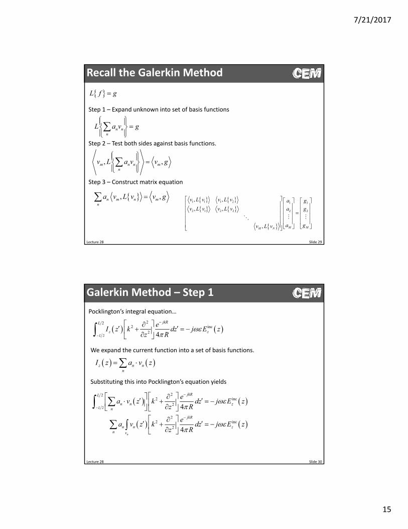
Lecture 28 Slide 29
Recall the Galerkin Method
Step 1 – Expand unknown into set of basis functions
L f g
n nn
L a v g
Step 2 – Test both sides against basis functions.
, ,m n n mn
v L a v v g
Step 3 – Construct matrix equation
, ,n m n mn
a v L v v g
1 1 1 2 1 1
2 1 2 2 2 2
, ,
, ,
, M MM N
v L v v L v a g
v L v v L v a g
a gv L v
Lecture 28 Slide 30
Galerkin Method – Step 1
We expand the current function into a set of basis functions.
z n nn
I z a v z Substituting this into Pocklington’s equation yields
2
222 inc
2 4L
jkRL
z z
eI z k dz j E z
z R
Pocklington’s integral equation…
2
222 inc
2
22 inc
2
4
4n
L
jkRL
n n zn
jkR
n n zn v
ea v z k dz j E z
z R
ea v z k dz j E z
z R
7/21/2017
16
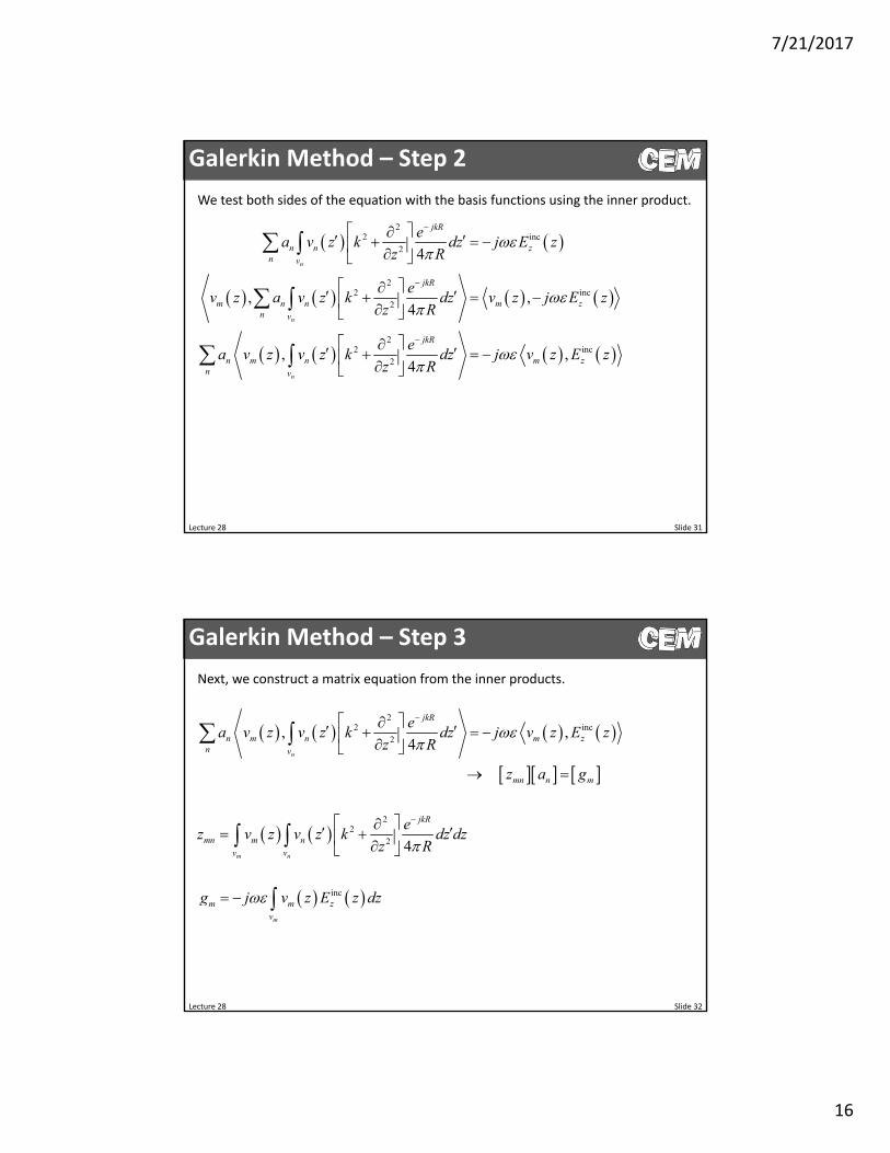
Lecture 28 Slide 31
Galerkin Method – Step 2
We test both sides of the equation with the basis functions using the inner product.
22 inc
2
22 inc
2
22 inc
2
4
, ,4
, ,4
n
n
n
jkR
n n zn v
jkR
m n n m zn v
jkR
n m n m zn v
ea v z k dz j E z
z R
ev z a v z k dz v z j E z
z R
ea v z v z k dz j v z E z
z R
Lecture 28 Slide 32
Galerkin Method – Step 3
Next, we construct a matrix equation from the inner products.
22 inc
2, ,
4
n
jkR
n m n m zn v
mn n m
ea v z v z k dz j v z E z
z R
z a g
2
22 4
m n
jkR
mn m n
v v
ez v z v z k dz dz
z R
inc
m
m m z
v
g j v z E z dz

7/21/2017
17
Lecture 28 Slide 33
Pulse Basis Functions (1 of 3)
We let our basis functions be pulse functions defined only on the segments.
th
th
0 is outside segment
1 is inside segmentm
z mv z
z m
Using these basis functions, we have
22
2
2 22
3
22
4
1
4
m n
m m
mm
jkR
mn m n
v v
z zz z zjkRjkr
mzz z zz
ez v z v z k dz dz
z R
e jkRk dz z z e
R R
inc
inc
m
m m z
v
z m
g j v z E z dz
j E z
2 2mR z z a
1v z 2v z 3v z 4v z 5v z
This is called point‐matching.
Lecture 28 Slide 34
Pulse Basis Functions (2 of 3)
When calculating the impedance elements, we must evaluate the following integral as part of those calculations.
2
2
4
n
n
zz
jkR
zz
edz
R
2 2mR z z a
When m = n, we can use a small argument approximation.
222
22
2
1 2 11 1ln
4 4 4 41 2 1
m
m
zz zjkR
z zz
a ze jkR jk zdz dz
R R a z
Otherwise, we must numerically evaluate the integral.

7/21/2017
18
Lecture 28 Slide 35
Pulse Basis Functions (3 of 3)
1i2i
3i4i
5i6i
7i1v
2v3v
4v5v
6v7v
mn n m
a i
z a g
We can now interpret [a] as a column vector containing the currents in each segment of the antenna.
Lecture 28 Slide 36
Transformation to True Impedance Matrix
The matrix equation is
mn n mz a g
The an coefficients are the currents in each segment. The gm coefficients are scaled electric fields. Based on this, it is more intuitive to write the matrix equation as
incmn n z mz i j E z
We would like the units on the right‐hand side to be voltage so that the [Z] matrix is true impedance. Voltage is related to the electric field through
inc mz m
VE z
z
The final matrix equation in terms of element voltage and current is
mn n m
j zz i V
True
mn n m
j zz i V
k
Z
7/21/2017
19
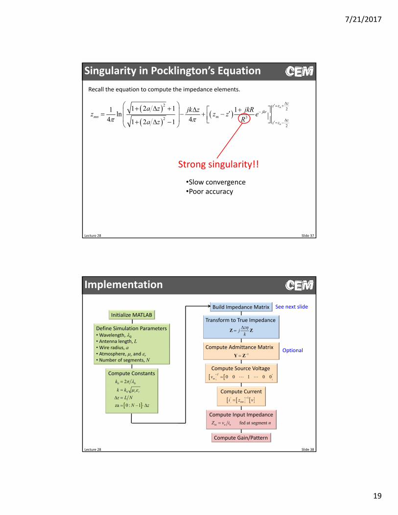
Lecture 28 Slide 37
Singularity in Pocklington’s Equation
Recall the equation to compute the impedance elements.
2
2
32
2
1 2 11 1ln
4 41 2 1
n
n
zz z
jkrmn m
zz z
a z jk z jkRz z z e
Ra z
Strong singularity!!
•Slow convergence•Poor accuracy
Lecture 28 Slide 38
Implementation
Initialize MATLAB
Define Simulation Parameters•Wavelength, 0
• Antenna length, L•Wire radius, a• Atmosphere, r and r• Number of segments, N
Compute Constants
0 0
0
2
za 0 : 1
r r
k
k k
z L N
N z
Build Impedance Matrix
Transform to True Impedancez
jk
Z Z
Compute Admittance Matrix1Y Z
Compute Source Voltage
0 0 1 0 0T
mv
Compute Current
1
mni z v
Compute Input Impedance
in fed at segment n nZ v i n
Compute Gain/Pattern
See next slide
Optional
7/21/2017
20
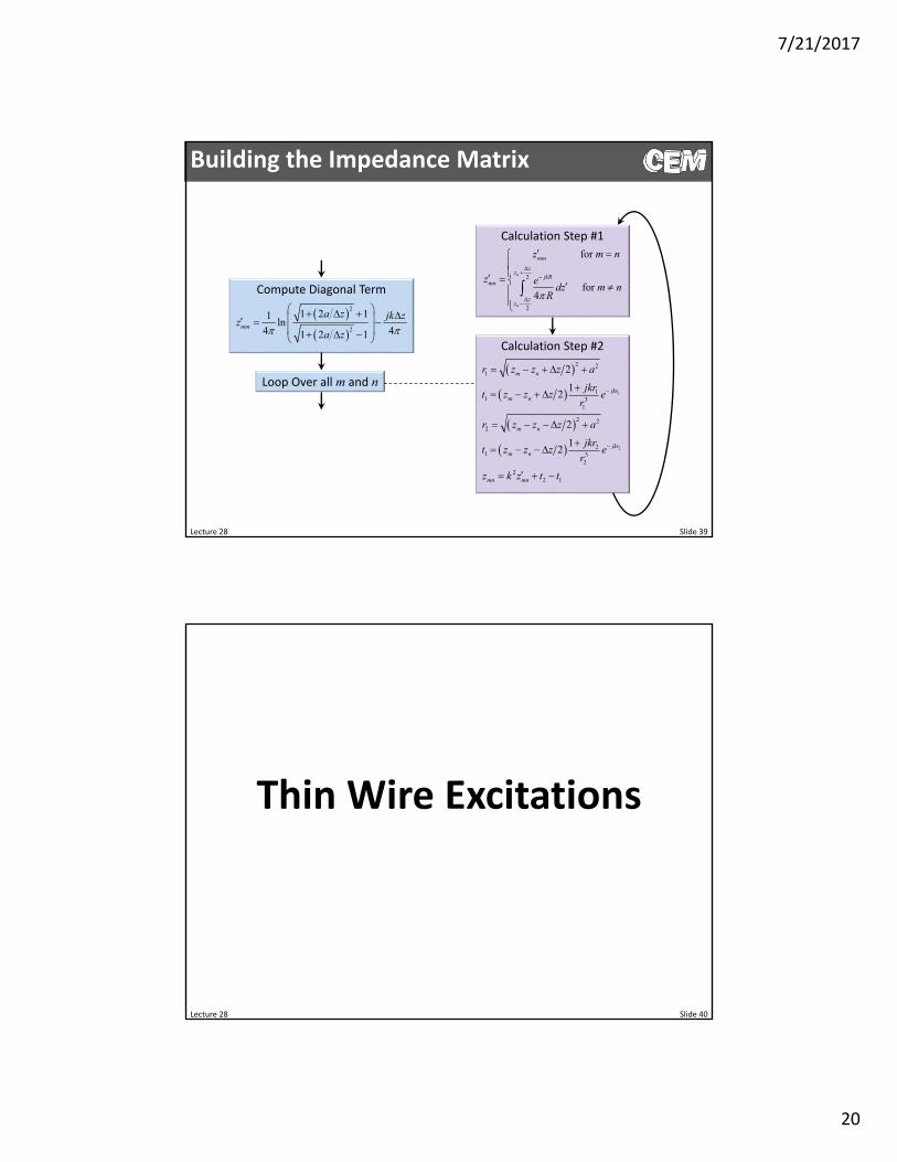
Lecture 28 Slide 39
Building the Impedance Matrix
Loop Over all m and n
Compute Diagonal Term
2
2
1 2 11ln
4 41 2 1mm
a z jk zz
a z
Calculation Step #1
2
2
for
for 4
n
n
mm
zz
jkRmn
zz
z m n
z edz m n
R
Calculation Step #2
1
2
2 21
11 3
1
2 22
21 3
2
22 1
2
12
2
12
m n
jkrm n
m n
jkrm n
mn mn
r z z z a
jkrt z z z e
r
r z z z a
jkrt z z z e
r
z k z t t
Lecture 28 Slide 40
Thin Wire Excitations

7/21/2017
21
Lecture 28 Slide 41
What is an Excitation?
Many antenna parameters are most easily calculated when the antenna is treated as a transmitting device.
The excitation of the antenna is the manner in which energy is “fed” into the antenna from an external source so that it can be radiated.
The properties of an antenna depend very much on how and where energy is applied to the structure.
The feed system of an antenna is a hugely complex subject so our approach will be to model the feed method and not the feed itself.
Feed network
Lecture 28 Slide 42
The Delta‐Gap Source
The detla‐gap source models the feed as if the incident field exists only in the small gap at the antenna terminals.
This is the simplest source to implement. It performs well for computing radiation patterns, but is usually less accurate for impedance calculations.
0v z
0inc ˆ at the gap
0 elsewherez
vz
E z z
7/21/2017
22
Lecture 28 Slide 43
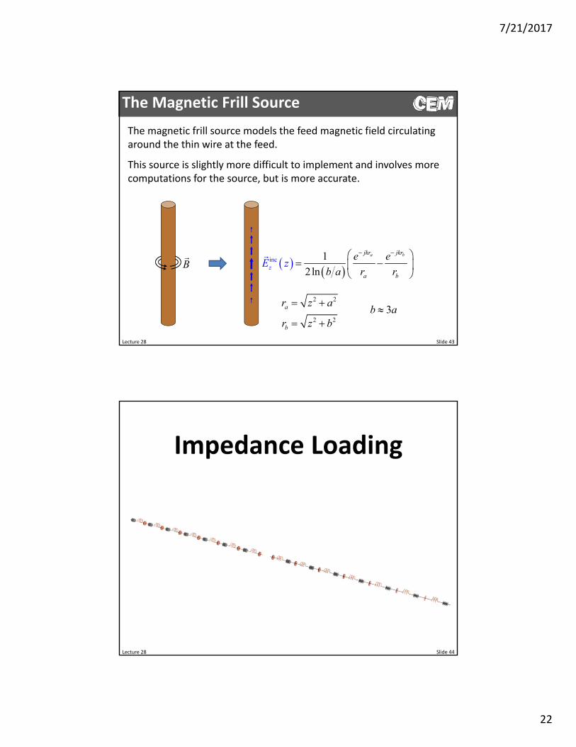
The Magnetic Frill Source
The magnetic frill source models the feed magnetic field circulating around the thin wire at the feed.
This source is slightly more difficult to implement and involves more computations for the source, but is more accurate.
B
2 2
2 2
a
b
r z a
r z b
inc 1
2ln
a bjkr
z
jkr
a b
e e
b a rE
rz
3b a
Lecture 28 Slide 44
Impedance Loading
7/21/2017
23
Method of
Moments
Lecture 28 Slide 45
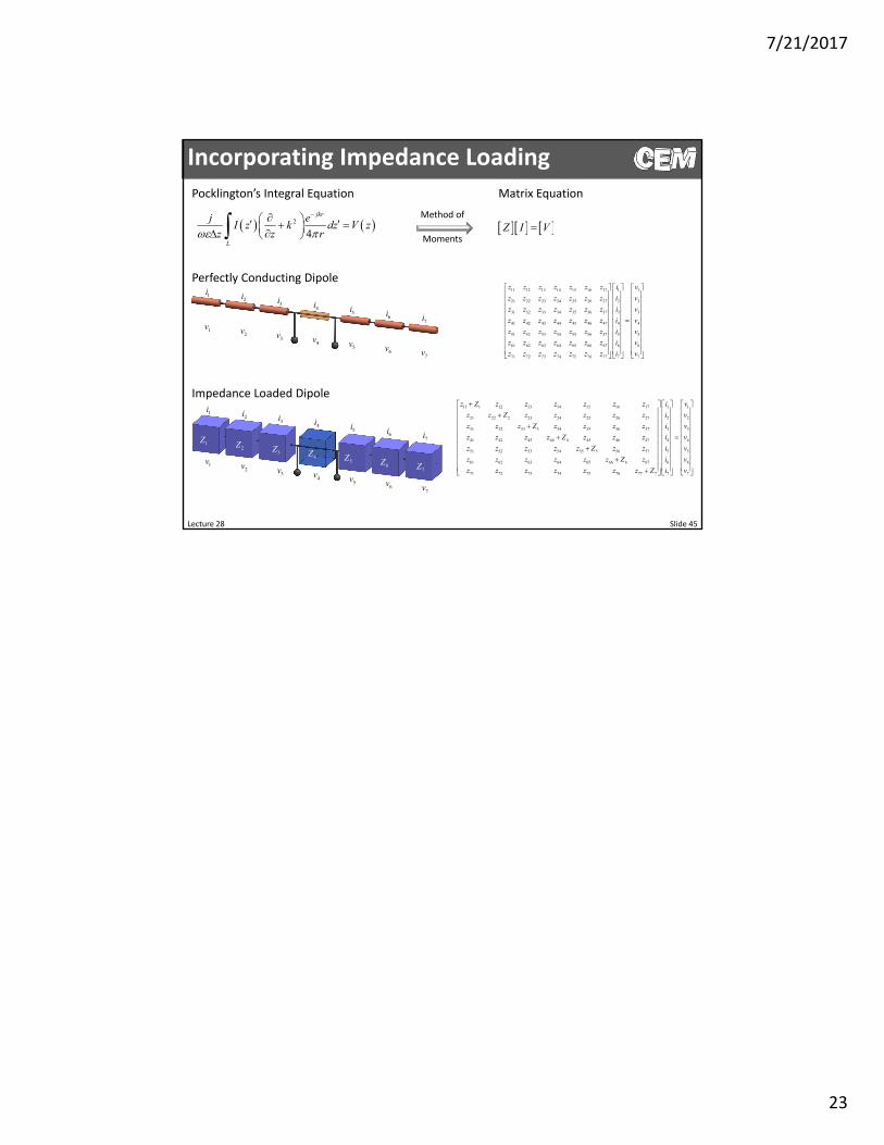
Incorporating Impedance LoadingPocklington’s Integral Equation
2
4
jkr
L
j eI z k dz V z
z z r
Z I V
Matrix Equation
11 12 13 14 15 16 17 1
21 22 23 24 25 26 27 2
31 32 33 34 35 36 37 3
41 42 43 44 45 46 47 4
51 52 53 54 55 56 57 5
61 62 63 64 65 66 67 6
71 72 73 74 75 76 77 7
z z z z z z z i
z z z z z z z i
z z z z z z z i
z z z z z z z i
z z z z z z z i
z z z z z z z i
z z z z z z z i
1
2
3
4
5
6
7
v
v
v
v
v
v
v
Perfectly Conducting Dipole
Impedance Loaded Dipole11 1 12 13 14 15 16 17 1
21 22 2 23 24 25 26 27 2
31 32 33 3 34 35 36 37 3
41 42 43 44 4 45 46 47 4
51 52 53 54 55 5 56 57 5
61 62 63 64 65 66 6 67
71 72 73 74 75 76 77 7
z Z z z z z z z i
z z Z z z z z z i
z z z Z z z z z i
z z z z Z z z z i
z z z z z Z z z i
z z z z z z Z z
z z z z z z z Z
1
2
3
4
5
6 6
7 7
v
v
v
v
v
i v
i v
1i2i
3i4i
5i6i
7i1v
2v3v
4v5v
6v7v
1i2i
3i4i
5i6i
7i
1v2v
3v4v
5v6v
7v
1Z2Z
3Z4Z
5Z6Z
7Z