Lecture 27

SERVO VALVES

Learning Objectives

Upon completion of this chapter, the student should be able to:

Define servo valve.

Compare servo valves with proportional valves.

Appreciate the history of servo valves.

Describe the working of a servo torque motor.

Describe the working of single-stage spool-type servo valves.

Describe the working of jet-type servo valves.

Analyze the valve performance.

Define dead band and hysteresis.

Analyze mathematically the simple servo systems.

1.1 Introduction

Servo valves were developed to facilitate the adjustment of fluid flow based on changes in the load

motion. Simply put, it is a programmable orifice.In machine motion control, servo systems involve

continuous monitoring, feedback and correction. Also they are used to improve efficiency, accuracy

and repeatability. The most common applications of servo valves are in aerospace vehicles,

particularly in primary flight controls. In aircraft, control surfaces such as ailerons, elevators and

rudders are positioned by servo units. In space vehicles, control during launch is provided by movable

thrust nozzles that are positioned by servo units. Even the drill bits for angle drilling of oil wells are

servo controlled.

A servomechanism is defined as an automatic device for controlling a large amount of power by

means of a very small amount of power and automatically correcting the performance of a

mechanism. The automatic and continuous correction requires return of information from the

mechanism– feedback, in other words. Therefore, a servo valve is operated without feedback and it is

not a true servomechanism. In Chapter 17 we have studied about proportional valves and Table 1.1

gives comparison between servo valve and electrohydraulic proportional control valves (EHPV).

Table 1.1 Comparison of servo valves and electrohydraulic proportional valves

Feature Servo Valve EHPV

Electrical operator Torque motor Proportional solenoid

Manufacturing precision Extremely high Moderately high

Feedback circuitry Main system as well as

valve

Valve (depending on type),

main system (seldom)

Cost (compared with a solenoid

valve)

Very expensive Moderately expensive

1.2 History of Electrohydraulic Servomechanisms

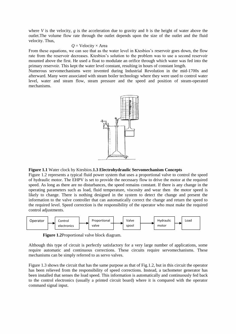
The earliest recognized servomechanism is the water clock invented around 250 BC(Fig. 1.1) by the

Alexandrian inventor Ktesbios. In this device, time was recorded by the level of water in a graduated

vessel. Water flows into the vessel at a controlled and constant rate from a water reservoir above it.

The control of the flow rate from the reservoir involves a mechanism.Velocity flow rate from the

outlet of a reservoir is determined by the equation

2v gh

where V is the velocity, g is the acceleration due to gravity and h is the height of water above the

outlet.The volume flow rate through the outlet depends upon the size of the outlet and the fluid

velocity. Thus,

Q = Velocity × Area

From these equations, we can see that as the water level in Ktesbios’s reservoir goes down, the flow

rate from the reservoir decreases. Ktesbios’s solution to the problem was to use a second reservoir

mounted above the first. He used a float to modulate an orifice through which water was fed into the

primary reservoir. This kept the water level constant, resulting in hours of constant length.

Numerous servomechanisms were invented during Industrial Revolution in the mid-1700s and

afterward. Many were associated with steam boiler technology where they were used to control water

level, water and steam flow, steam pressure and the speed and position of steam-operated

mechanisms.

Figure 1.1 Water clock by Ktesbios.1.3 Electrohydraulic Servomechanism Concepts

Figure 1.2 represents a typical fluid power system that uses a proportional valve to control the speed

of hydraulic motor. The EHPV is set to provide the necessary flow to drive the motor at the required

speed. As long as there are no disturbances, the speed remains constant. If there is any change in the

operating parameters such as load, fluid temperature, viscosity and wear then the motor speed is

likely to change. There is nothing designed in the system to detect the change and present the

information to the valve controller that can automatically correct the change and return the speed to

the required level. Speed correction is the responsibility of the operator who must make the required

control adjustments.

Figure 1.2Proportional valve block diagram.

Although this type of circuit is perfectly satisfactory for a very large number of applications, some

require automatic and continuous corrections. These circuits require servomechanisms. These

mechanisms can be simply referred to as servo valves.

Figure 1.3 shows the circuit that has the same purpose as that of Fig.1.2, but in this circuit the operator

has been relieved from the responsibility of speed corrections. Instead, a tachometer generator has

been installed that senses the load speed. This information is automatically and continuously fed back

to the control electronics (usually a printed circuit board) where it is compared with the operator

command signal input.

Operator Control

electronics

Proportional

valve

Valve

spool

Hydraulic

motor

Load

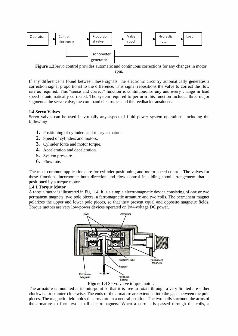
Figure 1.3Servo control provides automatic and continuous corrections for any changes in motor

rpm.

If any difference is found between these signals, the electronic circuitry automatically generates a

correction signal proportional to the difference. This signal repositions the valve to correct the flow

rate as required. This “sense and correct” function is continuous, so any and every change in load

speed is automatically corrected. The system required to perform this function includes three major

segments: the servo valve, the command electronics and the feedback transducer.

1.4 Servo Valves

Servo valves can be used in virtually any aspect of fluid power system operations, including the

following:

1. Positioning of cylinders and rotary actuators.

2. Speed of cylinders and motors.

3. Cylinder force and motor torque.

4. Acceleration and deceleration.

5. System pressure.

6. Flow rate.

The most common applications are for cylinder positioning and motor speed control. The valves for

these functions incorporate both direction and flow control in sliding spool arrangement that is

positioned by a torque motor.

1.4.1 Torque Motor

A torque motor is illustrated in Fig. 1.4. It is a simple electromagnetic device consisting of one or two

permanent magnets, two pole pieces, a ferromagnetic armature and two coils. The permanent magnet

polarizes the upper and lower pole pieces, so that they present equal and opposite magnetic fields.

Torque motors are very low-power devices operated on low-voltage DC power.

Figure 1.4 Servo valve torque motor.

The armature is mounted at its mid-point so that it is free to rotate through a very limited are either

clockwise or counter-clockwise. The ends of the armature are extended into the gaps between the pole

pieces. The magnetic field holds the armature in a neutral position. The two coils surround the arms of

the armature to form two small electromagnets. When a current is passed through the coils, a

Tachometer

generator

Operator Control

electronics

Proportion

al valve

Valve

spool

Hydraulic

motor

Load

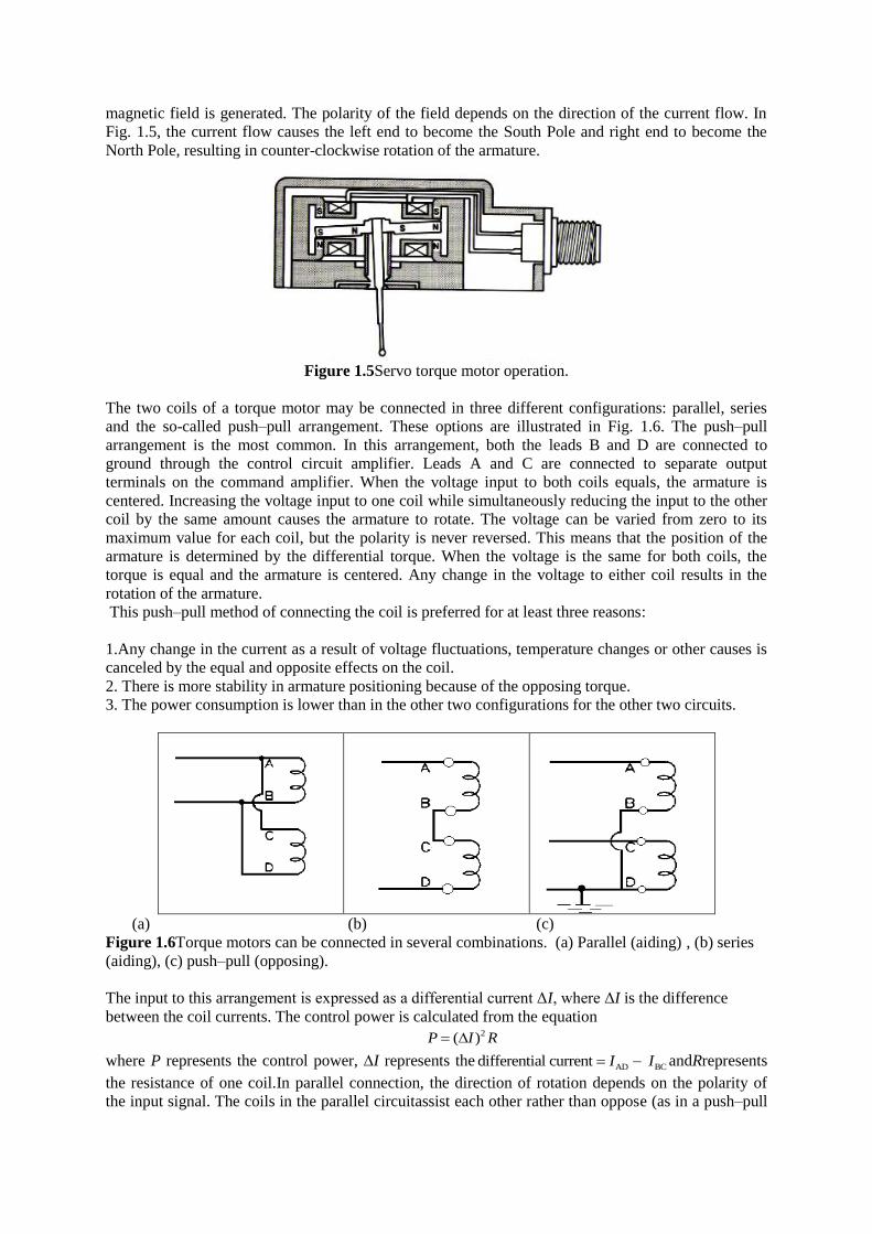
magnetic field is generated. The polarity of the field depends on the direction of the current flow. In

Fig. 1.5, the current flow causes the left end to become the South Pole and right end to become the

North Pole, resulting in counter-clockwise rotation of the armature.

Figure 1.5Servo torque motor operation.

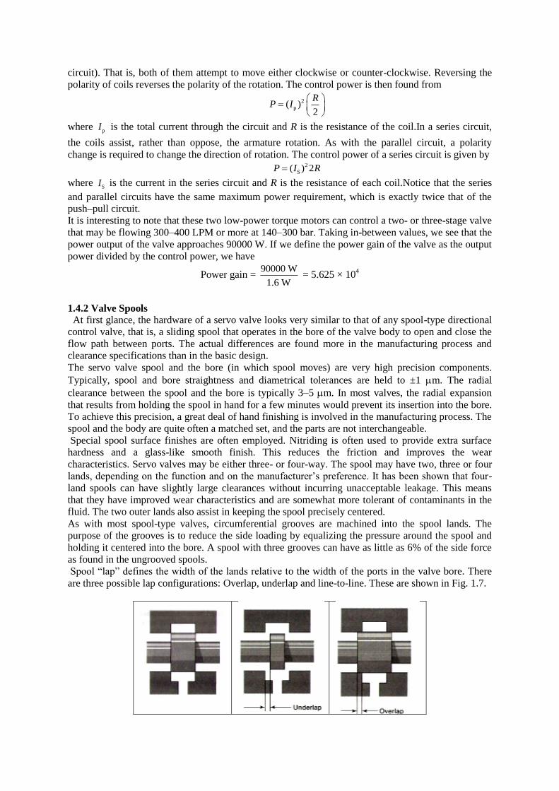
The two coils of a torque motor may be connected in three different configurations: parallel, series

and the so-called push–pull arrangement. These options are illustrated in Fig. 1.6. The push–pull

arrangement is the most common. In this arrangement, both the leads B and D are connected to

ground through the control circuit amplifier. Leads A and C are connected to separate output

terminals on the command amplifier. When the voltage input to both coils equals, the armature is

centered. Increasing the voltage input to one coil while simultaneously reducing the input to the other

coil by the same amount causes the armature to rotate. The voltage can be varied from zero to its

maximum value for each coil, but the polarity is never reversed. This means that the position of the

armature is determined by the differential torque. When the voltage is the same for both coils, the

torque is equal and the armature is centered. Any change in the voltage to either coil results in the

rotation of the armature.

This push–pull method of connecting the coil is preferred for at least three reasons:

1.Any change in the current as a result of voltage fluctuations, temperature changes or other causes is

canceled by the equal and opposite effects on the coil.

2. There is more stability in armature positioning because of the opposing torque.

3. The power consumption is lower than in the other two configurations for the other two circuits.

(a) (b) (c)

Figure 1.6Torque motors can be connected in several combinations. (a) Parallel (aiding) , (b) series

(aiding), (c) push–pull (opposing).

The input to this arrangement is expressed as a differential current ΔI, where ΔI is the difference

between the coil currents. The control power is calculated from the equation 2( )P I R

where P represents the control power, I represents theAD BCdifferential current  I I andRrepresents

the resistance of one coil.In parallel connection, the direction of rotation depends on the polarity of

the input signal. The coils in the parallel circuitassist each other rather than oppose (as in a push–pull

circuit). That is, both of them attempt to move either clockwise or counter-clockwise. Reversing the

polarity of coils reverses the polarity of the rotation. The control power is then found from

2

p( )2

RP I

where pI is the total current through the circuit and R is the resistance of the coil.In a series circuit,

the coils assist, rather than oppose, the armature rotation. As with the parallel circuit, a polarity

change is required to change the direction of rotation. The control power of a series circuit is given by 2

S( ) 2P I R

where SI is the current in the series circuit and R is the resistance of each coil.Notice that the series

and parallel circuits have the same maximum power requirement, which is exactly twice that of the

push–pull circuit.

It is interesting to note that these two low-power torque motors can control a two- or three-stage valve

that may be flowing 300–400 LPM or more at 140–300 bar. Taking in-between values, we see that the

power output of the valve approaches 90000 W. If we define the power gain of the valve as the output

power divided by the control power, we have

Power gain = 90000 W

1.6 W = 5.625 × 10

4

1.4.2 Valve Spools

At first glance, the hardware of a servo valve looks very similar to that of any spool-type directional

control valve, that is, a sliding spool that operates in the bore of the valve body to open and close the

flow path between ports. The actual differences are found more in the manufacturing process and

clearance specifications than in the basic design.

The servo valve spool and the bore (in which spool moves) are very high precision components.

Typically, spool and bore straightness and diametrical tolerances are held to ±1 m. The radial

clearance between the spool and the bore is typically 3–5 m. In most valves, the radial expansion

that results from holding the spool in hand for a few minutes would prevent its insertion into the bore.

To achieve this precision, a great deal of hand finishing is involved in the manufacturing process. The

spool and the body are quite often a matched set, and the parts are not interchangeable.

Special spool surface finishes are often employed. Nitriding is often used to provide extra surface

hardness and a glass-like smooth finish. This reduces the friction and improves the wear

characteristics. Servo valves may be either three- or four-way. The spool may have two, three or four

lands, depending on the function and on the manufacturer’s preference. It has been shown that four-

land spools can have slightly large clearances without incurring unacceptable leakage. This means

that they have improved wear characteristics and are somewhat more tolerant of contaminants in the

fluid. The two outer lands also assist in keeping the spool precisely centered.

As with most spool-type valves, circumferential grooves are machined into the spool lands. The

purpose of the grooves is to reduce the side loading by equalizing the pressure around the spool and

holding it centered into the bore. A spool with three grooves can have as little as 6% of the side force

as found in the ungrooved spools.

Spool “lap” defines the width of the lands relative to the width of the ports in the valve bore. There

are three possible lap configurations: Overlap, underlap and line-to-line. These are shown in Fig. 1.7.

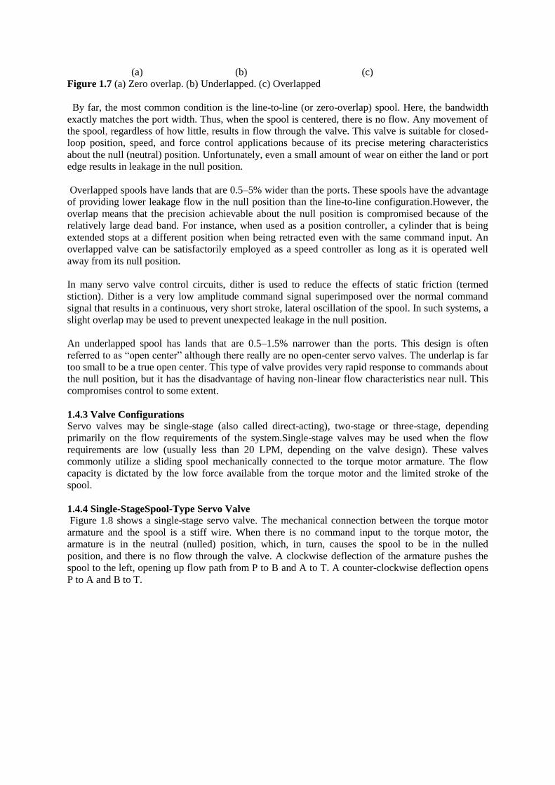
(a) (b) (c)

Figure 1.7 (a) Zero overlap. (b) Underlapped. (c) Overlapped

By far, the most common condition is the line-to-line (or zero-overlap) spool. Here, the bandwidth

exactly matches the port width. Thus, when the spool is centered, there is no flow. Any movement of

the spool, regardless of how little, results in flow through the valve. This valve is suitable for closed-

loop position, speed, and force control applications because of its precise metering characteristics

about the null (neutral) position. Unfortunately, even a small amount of wear on either the land or port

edge results in leakage in the null position.

Overlapped spools have lands that are 0.5–5% wider than the ports. These spools have the advantage

of providing lower leakage flow in the null position than the line-to-line configuration.However, the

overlap means that the precision achievable about the null position is compromised because of the

relatively large dead band. For instance, when used as a position controller, a cylinder that is being

extended stops at a different position when being retracted even with the same command input. An

overlapped valve can be satisfactorily employed as a speed controller as long as it is operated well

away from its null position.

In many servo valve control circuits, dither is used to reduce the effects of static friction (termed

stiction). Dither is a very low amplitude command signal superimposed over the normal command

signal that results in a continuous, very short stroke, lateral oscillation of the spool. In such systems, a

slight overlap may be used to prevent unexpected leakage in the null position.

An underlapped spool has lands that are 0.5–1.5% narrower than the ports. This design is often

referred to as “open center” although there really are no open-center servo valves. The underlap is far

too small to be a true open center. This type of valve provides very rapid response to commands about

the null position, but it has the disadvantage of having non-linear flow characteristics near null. This

compromises control to some extent.

1.4.3 Valve Configurations

Servo valves may be single-stage (also called direct-acting), two-stage or three-stage, depending

primarily on the flow requirements of the system.Single-stage valves may be used when the flow

requirements are low (usually less than 20 LPM, depending on the valve design). These valves

commonly utilize a sliding spool mechanically connected to the torque motor armature. The flow

capacity is dictated by the low force available from the torque motor and the limited stroke of the

spool.

1.4.4 Single-StageSpool-Type Servo Valve

Figure 1.8 shows a single-stage servo valve. The mechanical connection between the torque motor

armature and the spool is a stiff wire. When there is no command input to the torque motor, the

armature is in the neutral (nulled) position, which, in turn, causes the spool to be in the nulled

position, and there is no flow through the valve. A clockwise deflection of the armature pushes the

spool to the left, opening up flow path from P to B and A to T. A counter-clockwise deflection opens

P to A and B to T.

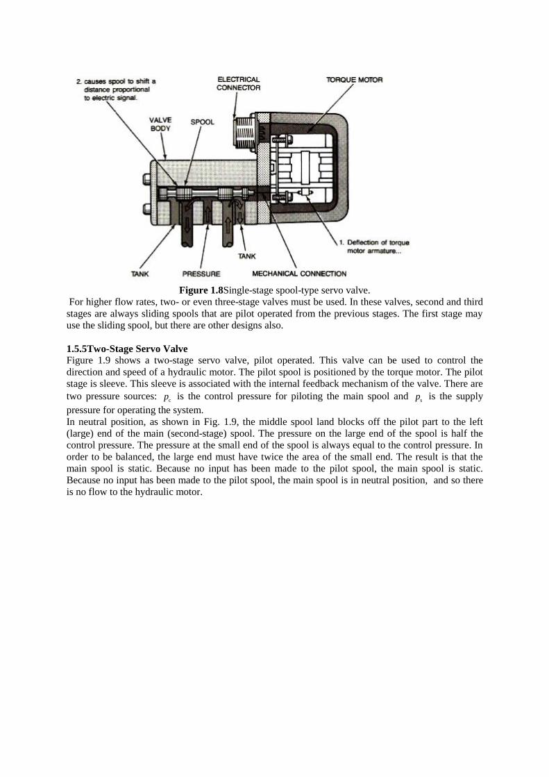
Figure 1.8Single-stage spool-type servo valve.

For higher flow rates, two- or even three-stage valves must be used. In these valves, second and third

stages are always sliding spools that are pilot operated from the previous stages. The first stage may

use the sliding spool, but there are other designs also.

1.5.5Two-Stage Servo Valve

Figure 1.9 shows a two-stage servo valve, pilot operated. This valve can be used to control the

direction and speed of a hydraulic motor. The pilot spool is positioned by the torque motor. The pilot

stage is sleeve. This sleeve is associated with the internal feedback mechanism of the valve. There are

two pressure sources: cp is the control pressure for piloting the main spool and

sp is the supply

pressure for operating the system.

In neutral position, as shown in Fig. 1.9, the middle spool land blocks off the pilot part to the left

(large) end of the main (second-stage) spool. The pressure on the large end of the spool is half the

control pressure. The pressure at the small end of the spool is always equal to the control pressure. In

order to be balanced, the large end must have twice the area of the small end. The result is that the

main spool is static. Because no input has been made to the pilot spool, the main spool is static.

Because no input has been made to the pilot spool, the main spool is in neutral position, and so there

is no flow to the hydraulic motor.

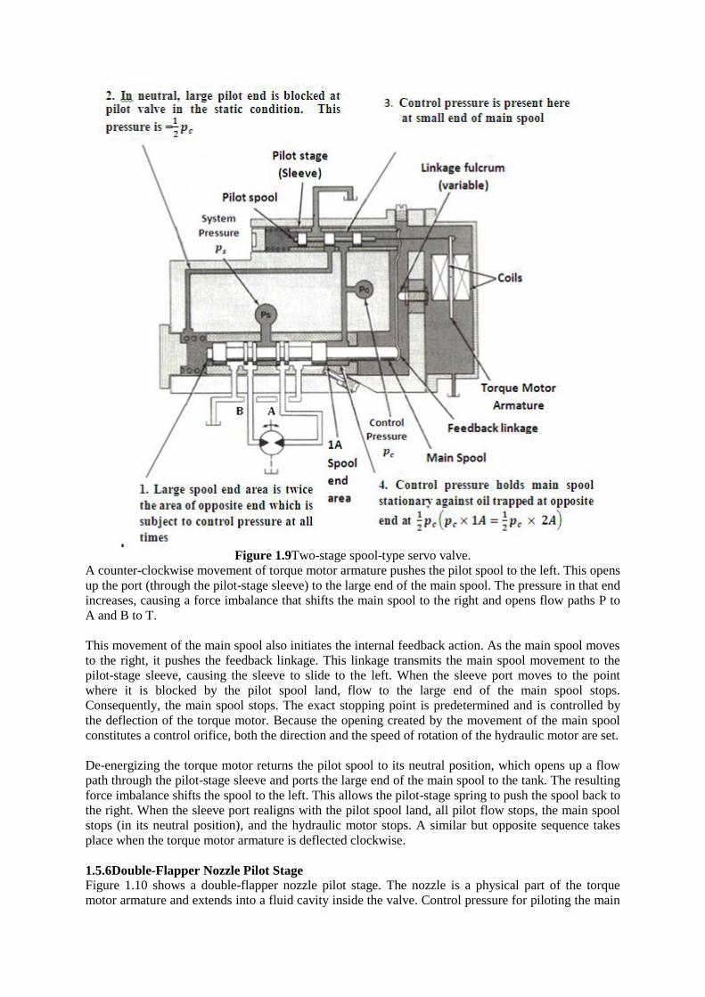
Figure 1.9Two-stage spool-type servo valve.

A counter-clockwise movement of torque motor armature pushes the pilot spool to the left. This opens

up the port (through the pilot-stage sleeve) to the large end of the main spool. The pressure in that end

increases, causing a force imbalance that shifts the main spool to the right and opens flow paths P to

A and B to T.

This movement of the main spool also initiates the internal feedback action. As the main spool moves

to the right, it pushes the feedback linkage. This linkage transmits the main spool movement to the

pilot-stage sleeve, causing the sleeve to slide to the left. When the sleeve port moves to the point

where it is blocked by the pilot spool land, flow to the large end of the main spool stops.

Consequently, the main spool stops. The exact stopping point is predetermined and is controlled by

the deflection of the torque motor. Because the opening created by the movement of the main spool

constitutes a control orifice, both the direction and the speed of rotation of the hydraulic motor are set.

De-energizing the torque motor returns the pilot spool to its neutral position, which opens up a flow

path through the pilot-stage sleeve and ports the large end of the main spool to the tank. The resulting

force imbalance shifts the spool to the left. This allows the pilot-stage spring to push the spool back to

the right. When the sleeve port realigns with the pilot spool land, all pilot flow stops, the main spool

stops (in its neutral position), and the hydraulic motor stops. A similar but opposite sequence takes

place when the torque motor armature is deflected clockwise.

1.5.6Double-Flapper Nozzle Pilot Stage

Figure 1.10 shows a double-flapper nozzle pilot stage. The nozzle is a physical part of the torque

motor armature and extends into a fluid cavity inside the valve. Control pressure for piloting the main

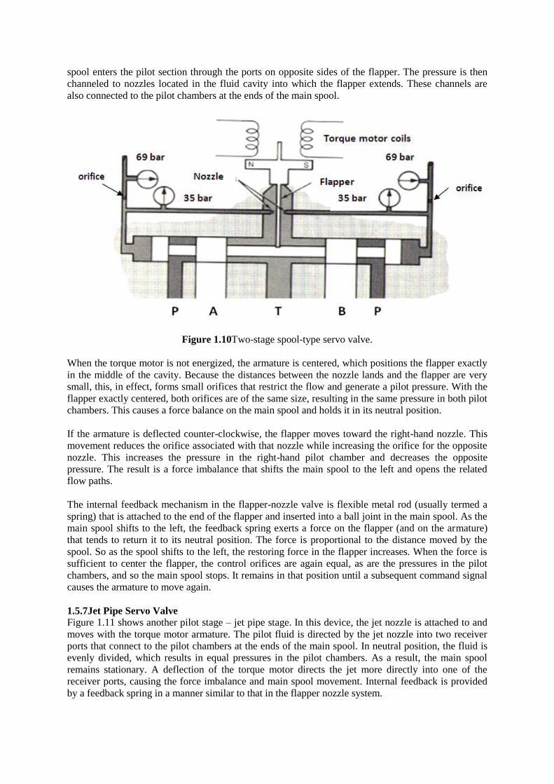
spool enters the pilot section through the ports on opposite sides of the flapper. The pressure is then

channeled to nozzles located in the fluid cavity into which the flapper extends. These channels are

also connected to the pilot chambers at the ends of the main spool.

Figure 1.10Two-stage spool-type servo valve.

When the torque motor is not energized, the armature is centered, which positions the flapper exactly

in the middle of the cavity. Because the distances between the nozzle lands and the flapper are very

small, this, in effect, forms small orifices that restrict the flow and generate a pilot pressure. With the

flapper exactly centered, both orifices are of the same size, resulting in the same pressure in both pilot

chambers. This causes a force balance on the main spool and holds it in its neutral position.

If the armature is deflected counter-clockwise, the flapper moves toward the right-hand nozzle. This

movement reduces the orifice associated with that nozzle while increasing the orifice for the opposite

nozzle. This increases the pressure in the right-hand pilot chamber and decreases the opposite

pressure. The result is a force imbalance that shifts the main spool to the left and opens the related

flow paths.

The internal feedback mechanism in the flapper-nozzle valve is flexible metal rod (usually termed a

spring) that is attached to the end of the flapper and inserted into a ball joint in the main spool. As the

main spool shifts to the left, the feedback spring exerts a force on the flapper (and on the armature)

that tends to return it to its neutral position. The force is proportional to the distance moved by the

spool. So as the spool shifts to the left, the restoring force in the flapper increases. When the force is

sufficient to center the flapper, the control orifices are again equal, as are the pressures in the pilot

chambers, and so the main spool stops. It remains in that position until a subsequent command signal

causes the armature to move again.

1.5.7Jet Pipe Servo Valve

Figure 1.11 shows another pilot stage – jet pipe stage. In this device, the jet nozzle is attached to and

moves with the torque motor armature. The pilot fluid is directed by the jet nozzle into two receiver

ports that connect to the pilot chambers at the ends of the main spool. In neutral position, the fluid is

evenly divided, which results in equal pressures in the pilot chambers. As a result, the main spool

remains stationary. A deflection of the torque motor directs the jet more directly into one of the

receiver ports, causing the force imbalance and main spool movement. Internal feedback is provided

by a feedback spring in a manner similar to that in the flapper nozzle system.

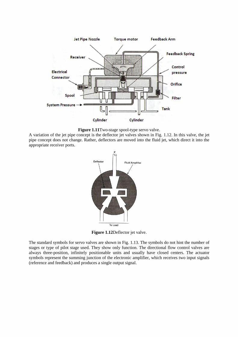
Figure 1.11Two-stage spool-type servo valve.

A variation of the jet pipe concept is the deflector jet valves shown in Fig. 1.12. In this valve, the jet

pipe concept does not change. Rather, deflectors are moved into the fluid jet, which direct it into the

appropriate receiver ports.

Figure 1.12Deflector jet valve.

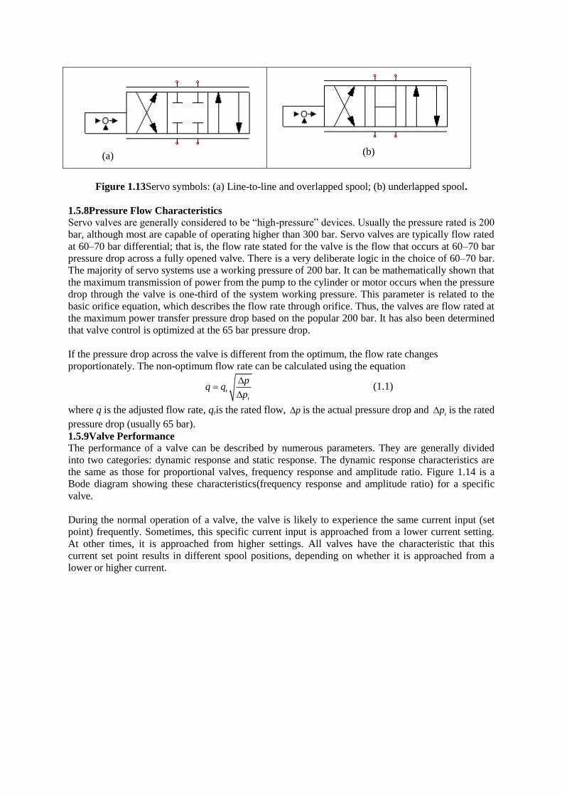
The standard symbols for servo valves are shown in Fig. 1.13. The symbols do not hint the number of

stages or type of pilot stage used. They show only function. The directional flow control valves are

always three-position, infinitely positionable units and usually have closed centers. The actuator

symbols represent the summing junction of the electronic amplifier, which receives two input signals

(reference and feedback) and produces a single output signal.

(a) (b)

Figure 1.13Servo symbols: (a) Line-to-line and overlapped spool; (b) underlapped spool.

1.5.8Pressure Flow Characteristics

Servo valves are generally considered to be “high-pressure” devices. Usually the pressure rated is 200

bar, although most are capable of operating higher than 300 bar. Servo valves are typically flow rated

at 60–70 bar differential; that is, the flow rate stated for the valve is the flow that occurs at 60–70 bar

pressure drop across a fully opened valve. There is a very deliberate logic in the choice of 60–70 bar.

The majority of servo systems use a working pressure of 200 bar. It can be mathematically shown that

the maximum transmission of power from the pump to the cylinder or motor occurs when the pressure

drop through the valve is one-third of the system working pressure. This parameter is related to the

basic orifice equation, which describes the flow rate through orifice. Thus, the valves are flow rated at

the maximum power transfer pressure drop based on the popular 200 bar. It has also been determined

that valve control is optimized at the 65 bar pressure drop.

If the pressure drop across the valve is different from the optimum, the flow rate changes

proportionately. The non-optimum flow rate can be calculated using the equation

r

r

pq q

p

(1.1)

where q is the adjusted flow rate, qris the rated flow, p is the actual pressure drop and rp is the rated

pressure drop (usually 65 bar).

1.5.9Valve Performance

The performance of a valve can be described by numerous parameters. They are generally divided

into two categories: dynamic response and static response. The dynamic response characteristics are

the same as those for proportional valves, frequency response and amplitude ratio. Figure 1.14 is a

Bode diagram showing these characteristics(frequency response and amplitude ratio) for a specific

valve.

During the normal operation of a valve, the valve is likely to experience the same current input (set

point) frequently. Sometimes, this specific current input is approached from a lower current setting.

At other times, it is approached from higher settings. All valves have the characteristic that this

current set point results in different spool positions, depending on whether it is approached from a

lower or higher current.

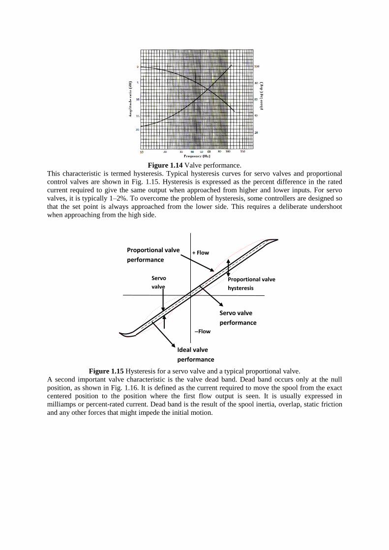
Figure 1.14 Valve performance.

This characteristic is termed hysteresis. Typical hysteresis curves for servo valves and proportional

control valves are shown in Fig. 1.15. Hysteresis is expressed as the percent difference in the rated

current required to give the same output when approached from higher and lower inputs. For servo

valves, it is typically 1–2%. To overcome the problem of hysteresis, some controllers are designed so

that the set point is always approached from the lower side. This requires a deliberate undershoot

when approaching from the high side.

Figure 1.15 Hysteresis for a servo valve and a typical proportional valve.

A second important valve characteristic is the valve dead band. Dead band occurs only at the null

position, as shown in Fig. 1.16. It is defined as the current required to move the spool from the exact

centered position to the position where the first flow output is seen. It is usually expressed in

milliamps or percent-rated current. Dead band is the result of the spool inertia, overlap, static friction

and any other forces that might impede the initial motion.

Proportional valve

hysteresis

Servo

valve

hysteresis

Proportional valve

performance

Servo valve

performance

+ Flow

Flow

Ideal valve

performance

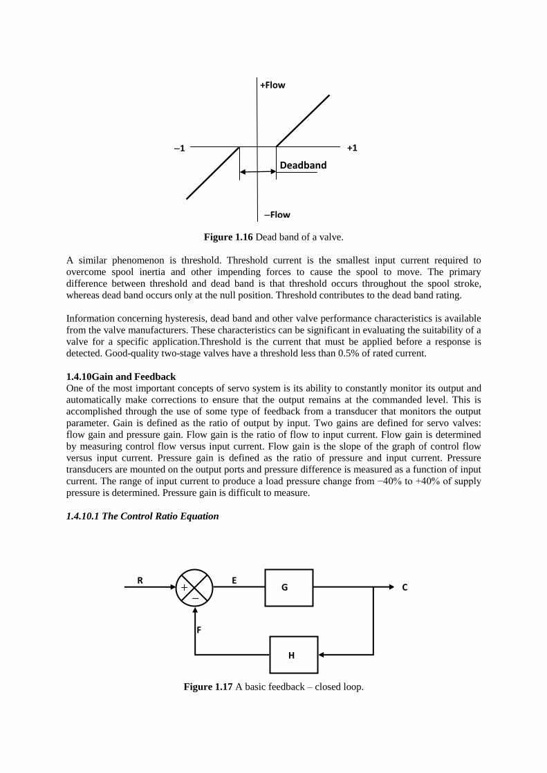
Figure 1.16 Dead band of a valve.

A similar phenomenon is threshold. Threshold current is the smallest input current required to

overcome spool inertia and other impending forces to cause the spool to move. The primary

difference between threshold and dead band is that threshold occurs throughout the spool stroke,

whereas dead band occurs only at the null position. Threshold contributes to the dead band rating.

Information concerning hysteresis, dead band and other valve performance characteristics is available

from the valve manufacturers. These characteristics can be significant in evaluating the suitability of a

valve for a specific application.Threshold is the current that must be applied before a response is

detected. Good-quality two-stage valves have a threshold less than 0.5% of rated current.

1.4.10Gain and Feedback

One of the most important concepts of servo system is its ability to constantly monitor its output and

automatically make corrections to ensure that the output remains at the commanded level. This is

accomplished through the use of some type of feedback from a transducer that monitors the output

parameter. Gain is defined as the ratio of output by input. Two gains are defined for servo valves:

flow gain and pressure gain. Flow gain is the ratio of flow to input current. Flow gain is determined

by measuring control flow versus input current. Flow gain is the slope of the graph of control flow

versus input current. Pressure gain is defined as the ratio of pressure and input current. Pressure

transducers are mounted on the output ports and pressure difference is measured as a function of input

current. The range of input current to produce a load pressure change from −40% to +40% of supply

pressure is determined. Pressure gain is difficult to measure.

1.4.10.1 The Control Ratio Equation

Figure 1.17 A basic feedback – closed loop.

F

E R

C G

H

+1 1

Deadband

+Flow

Flow

One of the most important aspects of system analysis is an understanding of system gain.Figure 1.17

is a block diagram of a generic system with feedback. The command input signal is given a designator

R for reference. The gain of the loop leg is designated G and termed the forward loop gain. The gain

of the feedback loop is denoted by H and the controlled output is shown as C.

As the system operates, a feedback signal F is continuously generated. Its value is based on the value

of C and the feedback gain. Thus,

   F CH

This feedback signal is fed to the summing junction (in the op-amp), where it is compared with the

reference signal. The result is an error signal E whose value is

– – E R F R CH (1.2)

This results in a change in the controlled variable C, which then becomes

   C EG (1.3)

and the process repeats itself.Equating Eqs. (1.2) and (1.3), we get

( – ) C R CH G – RG CGH

so that

            (1 )RG C CGH C GH

and, eventually,

   1

C G

R GH

(1.4)

This equation is known as the control ratio, and closed-loop gain or the closed-loop transfer function

of the system. The right-hand side of Eq. (1.4) defines the system gain and is commonly referred to as

the closed-loop gain of the system.

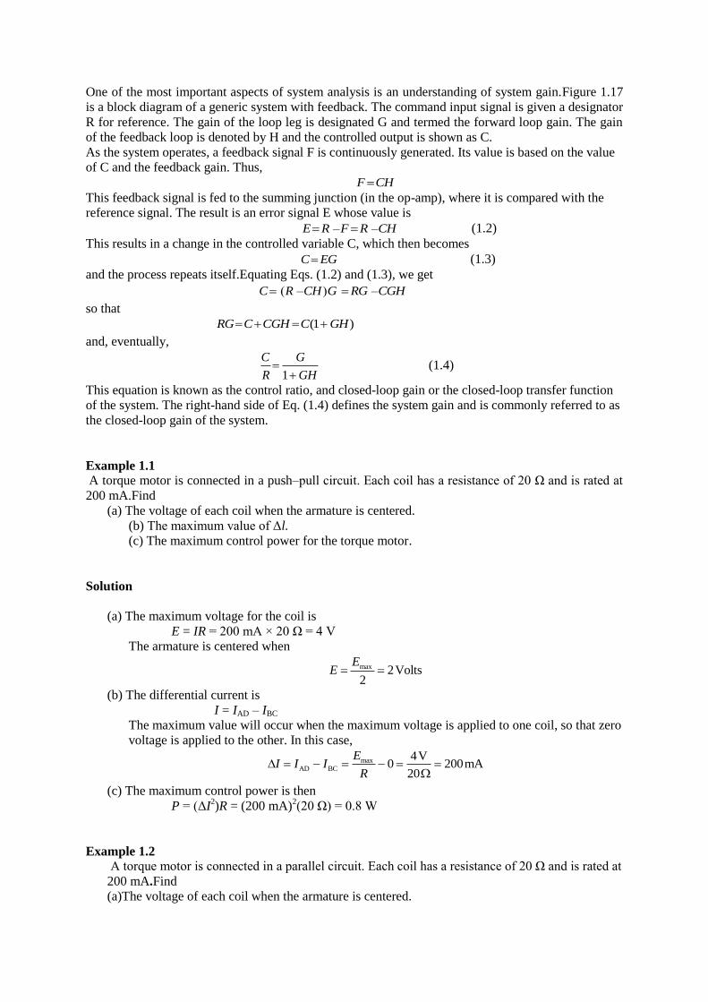
Example 1.1

A torque motor is connected in a push–pull circuit. Each coil has a resistance of 20 Ω and is rated at

200 mA.Find

(a) The voltage of each coil when the armature is centered.

(b) The maximum value of Δl.

(c) The maximum control power for the torque motor.

Solution

(a) The maximum voltage for the coil is

E = IR = 200 mA × 20 Ω = 4 V

The armature is centered when

max 2Volts2

EE

(b) The differential current is

I = IAD – IBC

The maximum value will occur when the maximum voltage is applied to one coil, so that zero

voltage is applied to the other. In this case,

max

AD BC

4V0 200mA

20

EI I I

R

(c) The maximum control power is then

P = (ΔI2)R = (200 mA)

2(20 Ω) = 0.8 W

Example 1.2

A torque motor is connected in a parallel circuit. Each coil has a resistance of 20 Ω and is rated at

200 mA.Find

(a)The voltage of each coil when the armature is centered.

(b) The maximum value of ΔI.

(c) The maximum control power for the torque motor

Solution: (a)The voltage to each coil will remain the same (4 V).

(b) The current through the circuit will increase because of lower resistance. For a parallel circuit

made up of two equal resistors, the equivalence resistance is R/2; in this case, 10 Ω.The value of I is

the total current, which we find from

P

4V0.4A=400mA

10

EI

R

(c) Control power is given by

P = (IP)2(R/2) = (400 mA)

2(20 Ω/2) = 1.6 W

Example 1.3

A torque motor is connected in a series circuit. Each coil has a resistance of 20 Ω and is rated at 200

mA. Find

(a)The voltage of each coil when the armature is centered.

(b) The maximum value of ΔI.

(c) The maximum control power for the torque motor

Solution: (a) A torque motor is connected in a series circuit. Therefore, total resistance is 2R or 40 Ω.

The maximum current will be 200 mA.

(b) A torque motor is connected in a series circuit thereforethe maximum voltage is

Voltage (E) = IR = (200 mA)(40 Ω) = 8 V

(c)The control power is

P = (Is)2 (2R) = (200 mA)

2(2)(20 Ω) = 1.6 W

Example 1.4

A servo valve is flow rated at 56 LPM at 65 bar differential (Fig. 1.5). It is to be operated in a 130 bar

system. What will its adjusted flow rate be at the optimum power transfer p?

Solution: For optimum power transfer, the pressure drop across the valve should be

130

3 = 43.33 bar

From Eq. (1.1), we have

q = qr

r

p

p

= 56

43.3

65= 45 LPM

example>

Example 1.5

Figure 1.18 shows a servo valve which is rated at 65 bar pressure drop across the valve in a 195 bar

system.

(a) Find the pressure drop when motor is fully loaded.

(b) Find the pressure drop when motor is not fully loaded.

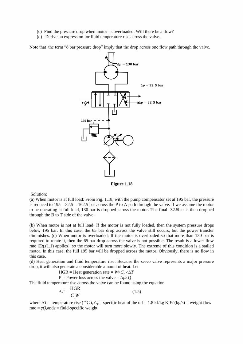
(c) Find the pressure drop when motor is overloaded. Will there be a flow?

(d) Derive an expression for fluid temperature rise across the valve.

Note that the term “6 bar pressure drop” imply that the drop across one flow path through the valve.

Figure 1.18

Solution:

(a) When motor is at full load: From Fig. 1.18, with the pump compensator set at 195 bar, the pressure

is reduced to 195 – 32.5 = 162.5 bar across the P to A path through the valve. If we assume the motor

to be operating at full load, 130 bar is dropped across the motor. The final 32.5bar is then dropped

through the B to T side of the valve.

(b) When motor is not at full load: If the motor is not fully loaded, then the system pressure drops

below 195 bar. In this case, the 65 bar drop across the valve still occurs, but the power transfer

diminishes. (c) When motor is overloaded: If the motor is overloaded so that more than 130 bar is

required to rotate it, then the 65 bar drop across the valve is not possible. The result is a lower flow

rate [Eq.(1.1) applies], so the motor will turn more slowly. The extreme of this condition is a stalled

motor. In this case, the full 195 bar will be dropped across the motor. Obviously, there is no flow in

this case.

(d) Heat generation and fluid temperature rise: Because the servo valve represents a major pressure

drop, it will also generate a considerable amount of heat. Let

HGR = Heat generation rate = WCp T

P = Power loss across the valve = pQ

The fluid temperature rise across the valve can be found using the equation

T = p

HGR

C W (1.5)

where T = temperature rise (    C ), Cp = specific heat of the oil = 1.8 kJ/kg K,W (kg/s) = weight flow

rate = γQ,andγ = fluid-specific weight.

195 bar

Example 1.5

For the servo valve of Example 1.5, determine the power loss, heat generation rate and the

temperature rise across the valve. The fluid has a specific weight of 8620 N/mm3.

Solution: The power loss is

P = Δp × q = 43.3×105 × (45/1000) × (1/60)

= 3.25 kW

The resultant heat generation rate is found from Eq.(1.5). The increase in the fluid temperature is

p     HGR /T C W

The weight flow rate is

   W Q

3

3

Oil flow rate in kg/s    (oil flow rate in m )

10895 45

60

0.67125 kg / s

/sQ

Therefore,

p   HGR /T C W

4.97   2.689  C

1.8 0.889

This is the temperature rise experienced by every drop of oil that flows through the valve. The rise

occurs in the time required for the fluid to flow through the portion of the valve where the pressure

drop occurs.

Although the weight flow rate appears in the equation, the temperature rise is actually independent of

flow rate. So the temperature rise for any fluid is a function of pressure drop only.

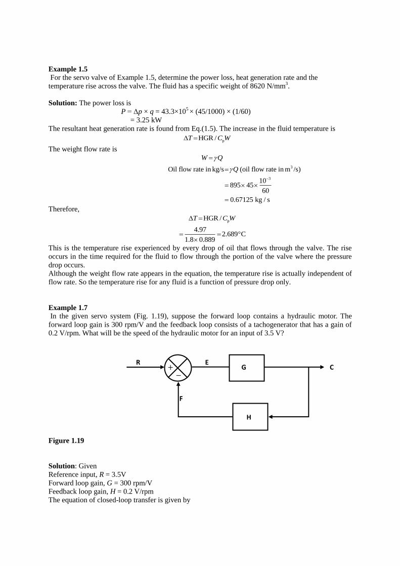
Example 1.7

In the given servo system (Fig. 1.19), suppose the forward loop contains a hydraulic motor. The

forward loop gain is 300 rpm/V and the feedback loop consists of a tachogenerator that has a gain of

0.2 V/rpm. What will be the speed of the hydraulic motor for an input of 3.5 V?

Figure 1.19

Solution: Given

Reference input, R = 3.5V

Forward loop gain, G = 300 rpm/V

Feedback loop gain, H = 0.2 V/rpm

The equation of closed-loop transfer is given by

F

E R

C G

H

C R

 1

C G

R GH

(1.6)

This gives

1

300(3.5)

1 300 0.2

17.2 rpm

GC R

GH

Normally, if the feedback system is not included, the 3.5 V input should give 1050 rpm. Because there

is feedback, the output is 17.6 rpm.

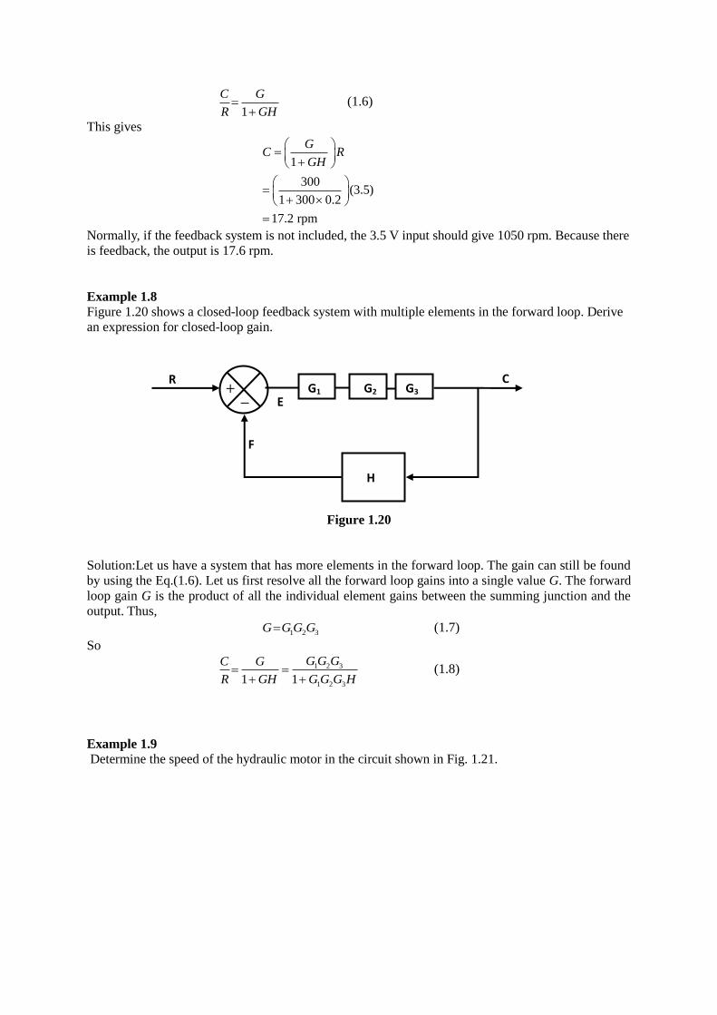
Example 1.8

Figure 1.20 shows a closed-loop feedback system with multiple elements in the forward loop. Derive

an expression for closed-loop gain.

Figure 1.20

Solution:Let us have a system that has more elements in the forward loop. The gain can still be found

by using the Eq.(1.6). Let us first resolve all the forward loop gains into a single value G. The forward

loop gain G is the product of all the individual element gains between the summing junction and the

output. Thus,

1 2 3   G G G G (1.7)

So

1 2 3

1 2 3

 1 1

G G GC G

R GH G G G H

(1.8)

Example 1.9

Determine the speed of the hydraulic motor in the circuit shown in Fig. 1.21.

E G1

F

R

C

H

G2 G3

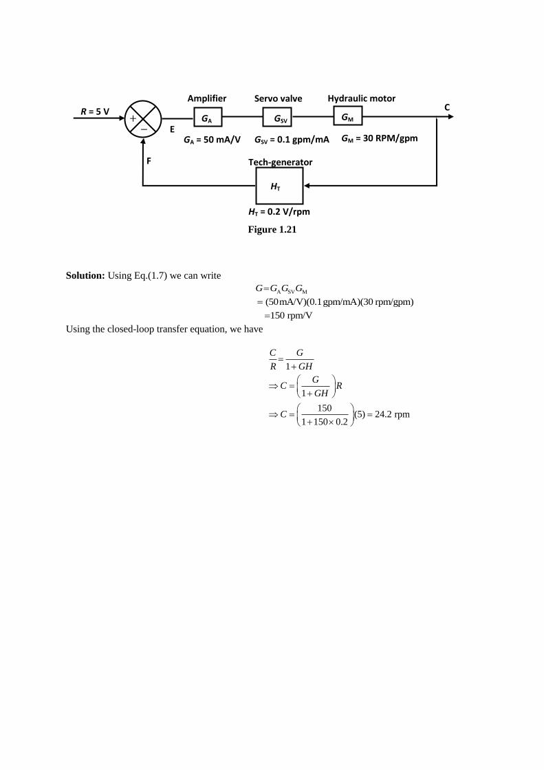
Figure 1.21

Solution: Using Eq.(1.7) we can write

A SV M   G G G G

 (50 mA/V)(0.1gpm/mA)(30 rpm/gpm)

1  50 rpm/V

Using the closed-loop transfer equation, we have

 1

1

150(5) 24.2 rpm

1 150 0.2

C G

R GH

GC R

GH

C

HT = 0.2 V/rpm

Tech-generator

Servo valve Hydraulic motor

Valve

Amplifier

E

F

R = 5 V

GA

C

HT

GSV GM

GA = 50 mA/V GSV = 0.1 gpm/mA

mA/V

GM = 30 RPM/gpm

mA/V

Objective-Type Questions

Fill in the Blanks

1. A servomechanism is defined as an automatic device for controlling a large amount of power by

means of a very small amount of _______.

2. Servo valves are operated by _______ motors.

3. Typically, spool and bore straightness and diametrical tolerances are held to _______.

4. Overlapped spools have lands that are 0.5% to _______% wider than the ports.

5. In many servo valve control circuits, _______ is used to reduce the effects of static friction (termed

stiction).

6. ______ valves may be used where the flow requirements usually less than 20 LPM_______.

State True or False

1. Servo valves are less expensive than proportional valves.

2. There is no dead zone for a servo valve.

3. A servo valve uses always zero or underlap spool.

4. The maximum operating frequency of a servo valve is 10 Hz.

5. Servo that uses feedback electronics is more accurate.

Review Questions

1. Define a servo valve.

2. How do servo valves differ from proportional control valves?

3. Explain the operation of a torque motor.

4. Define underlap, overlap and line to line in the context of servo valve spools.

5. Define dead band.

6. Define threshold.

7. Define hysteresis.

8. List and define the types of hydraulic amplifiers.

9. At what pressure drop are servo valves usually rated?

10. Define gain.

11. Define flow gain.

12. Define pressure gain.

13. What are the uses of servo valves?

14. What is a torque motor?

15. What is a spool lap?

16. What are the three types of servo valves?

Answers

Fill in the Blanks

1. Power

2. Torque

3. ±1 m

4. 5%

5. Dither

6. single stage

State True or False

1. False

2. False

3. False

4. True

5. True