Embed Size (px)
Citation preview
Lecture 27Exam 3 Review
Mark Hasegawa-JohnsonMay 3, 2021
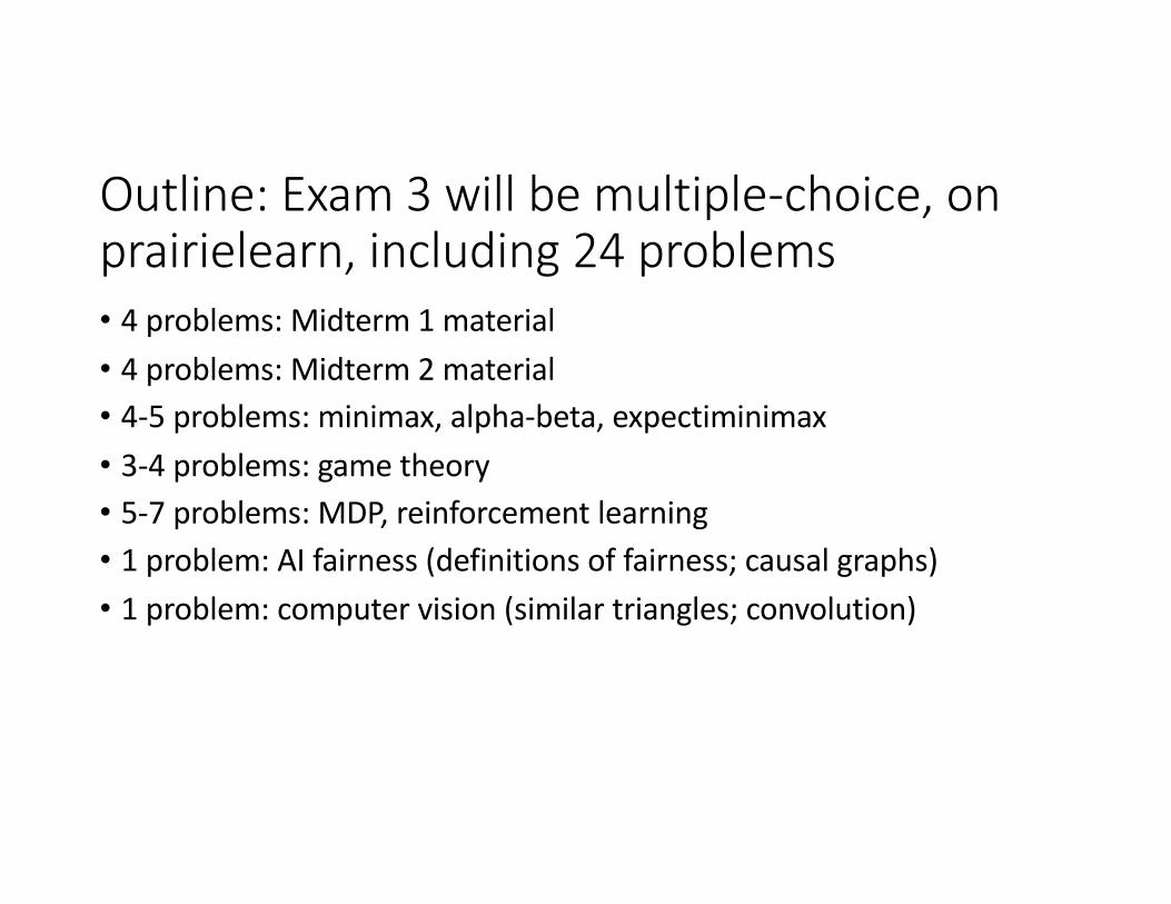
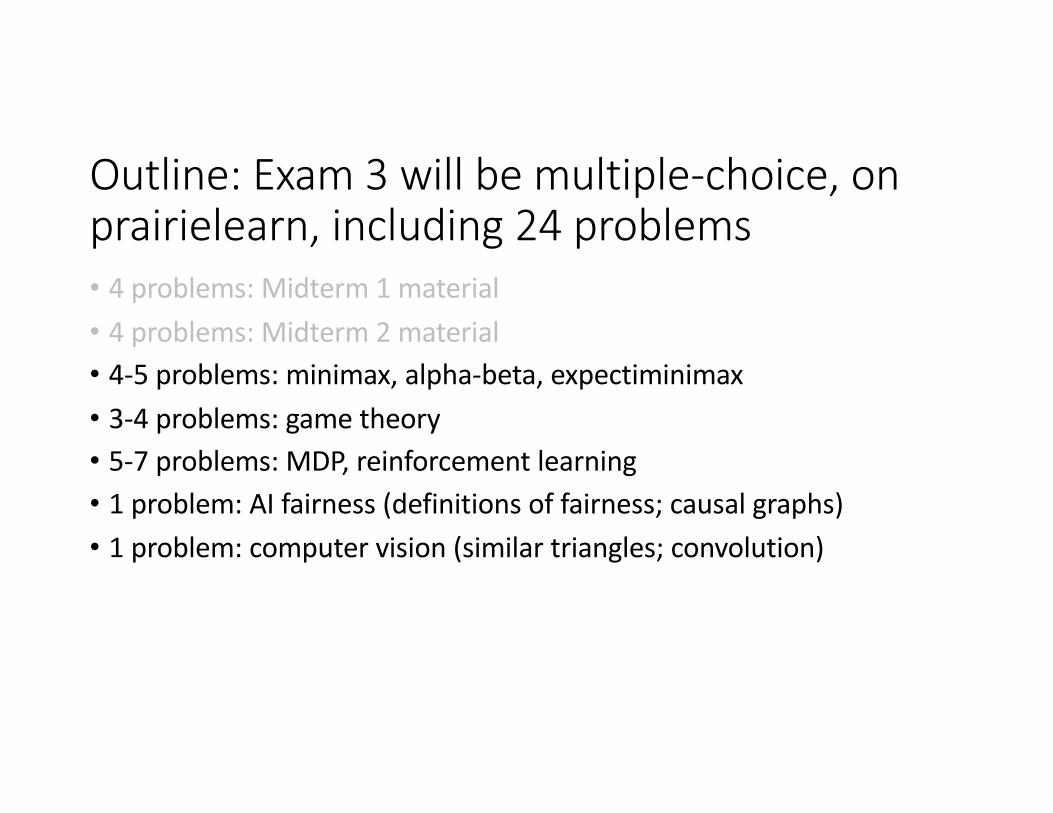
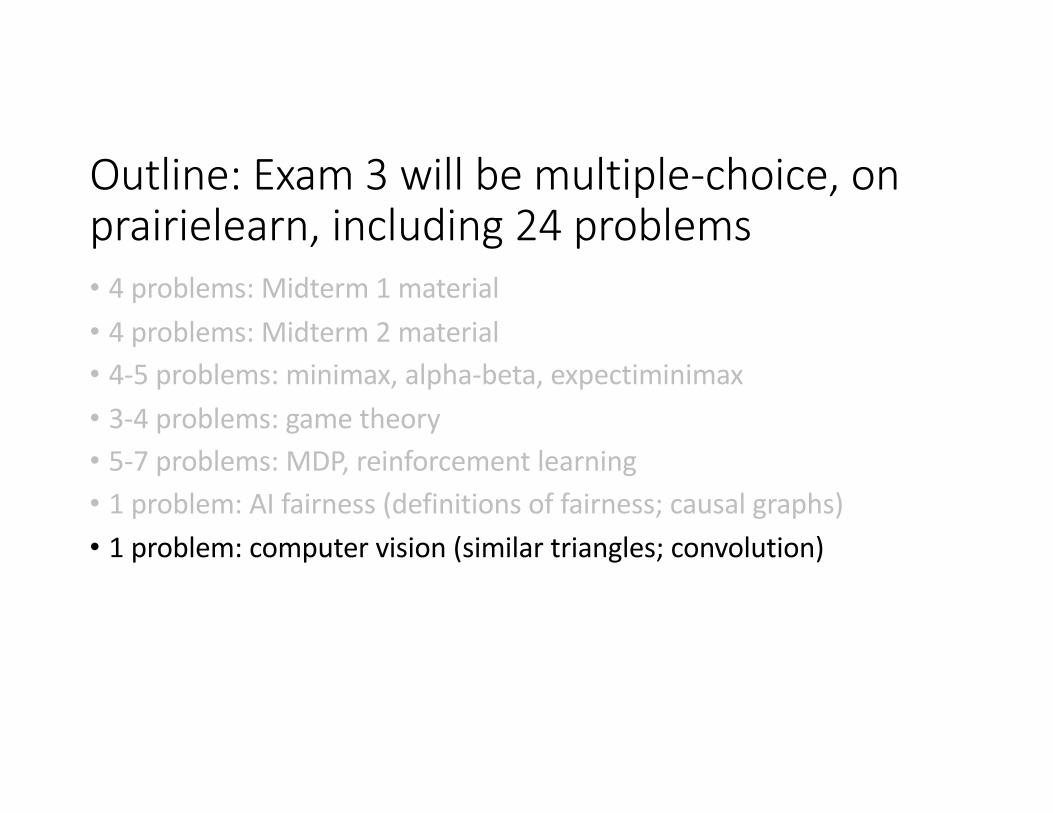
Outline: Exam 3 will be multiple-choice, on prairielearn, including 24 problems• 4 problems: Midterm 1 material• 4 problems: Midterm 2 material• 4-5 problems: minimax, alpha-beta, expectiminimax• 3-4 problems: game theory• 5-7 problems: MDP, reinforcement learning• 1 problem: AI fairness (definitions of fairness; causal graphs)• 1 problem: computer vision (similar triangles; convolution)
Outline: Exam 3 will be multiple-choice, on prairielearn, including 24 problems• 4 problems: Midterm 1 material• 4 problems: Midterm 2 material• 4-5 problems: minimax, alpha-beta, expectiminimax• 3-4 problems: game theory• 5-7 problems: MDP, reinforcement learning• 1 problem: AI fairness (definitions of fairness; causal graphs)• 1 problem: computer vision (similar triangles; convolution)
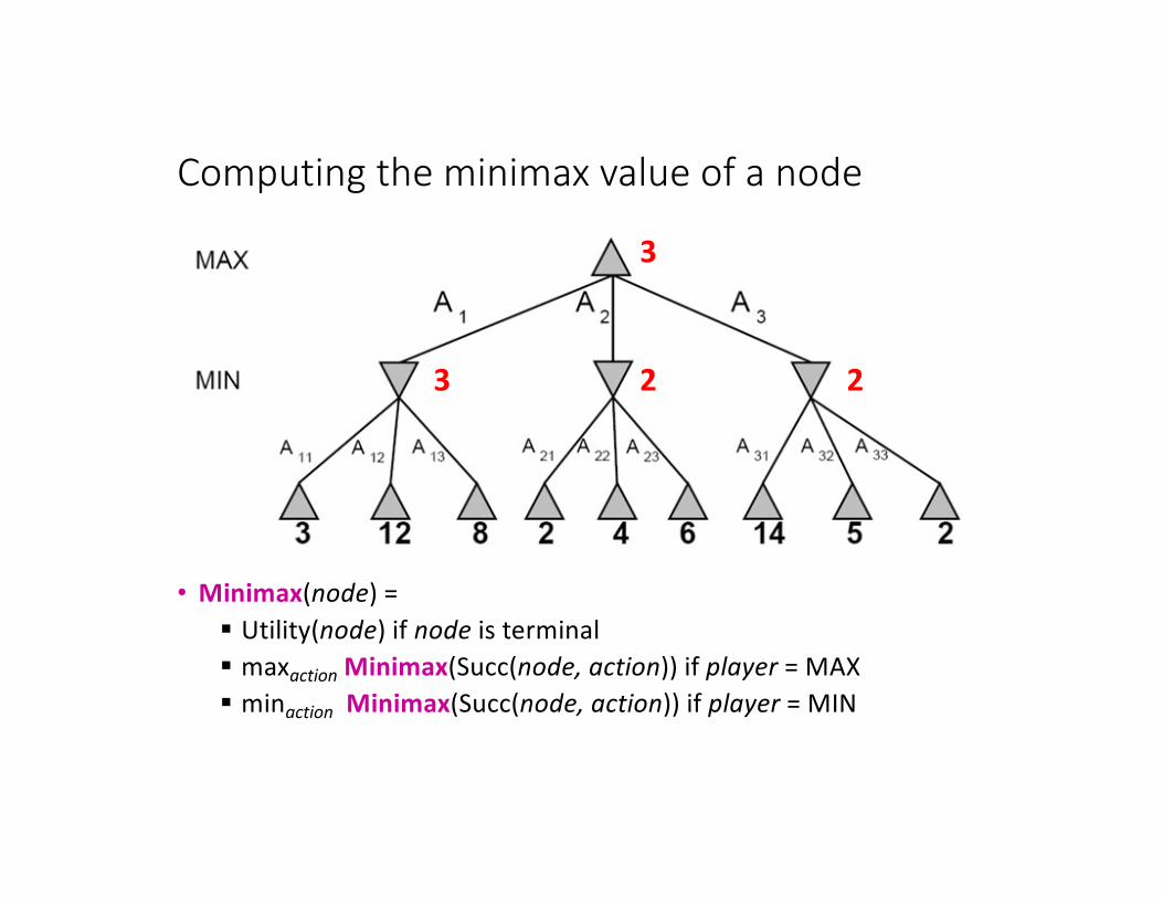
Computing the minimax value of a node
• Minimax(node) = § Utility(node) if node is terminal§ maxaction Minimax(Succ(node, action)) if player = MAX§ minaction Minimax(Succ(node, action)) if player = MIN
3 2 2
3
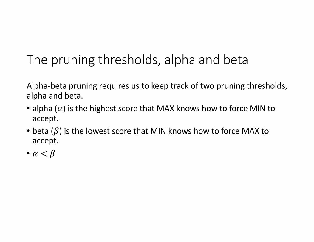
The pruning thresholds, alpha and beta
Alpha-beta pruning requires us to keep track of two pruning thresholds, alpha and beta.• alpha (𝛼) is the highest score that MAX knows how to force MIN to
accept.• beta (𝛽) is the lowest score that MIN knows how to force MAX to
accept.• 𝛼 < 𝛽
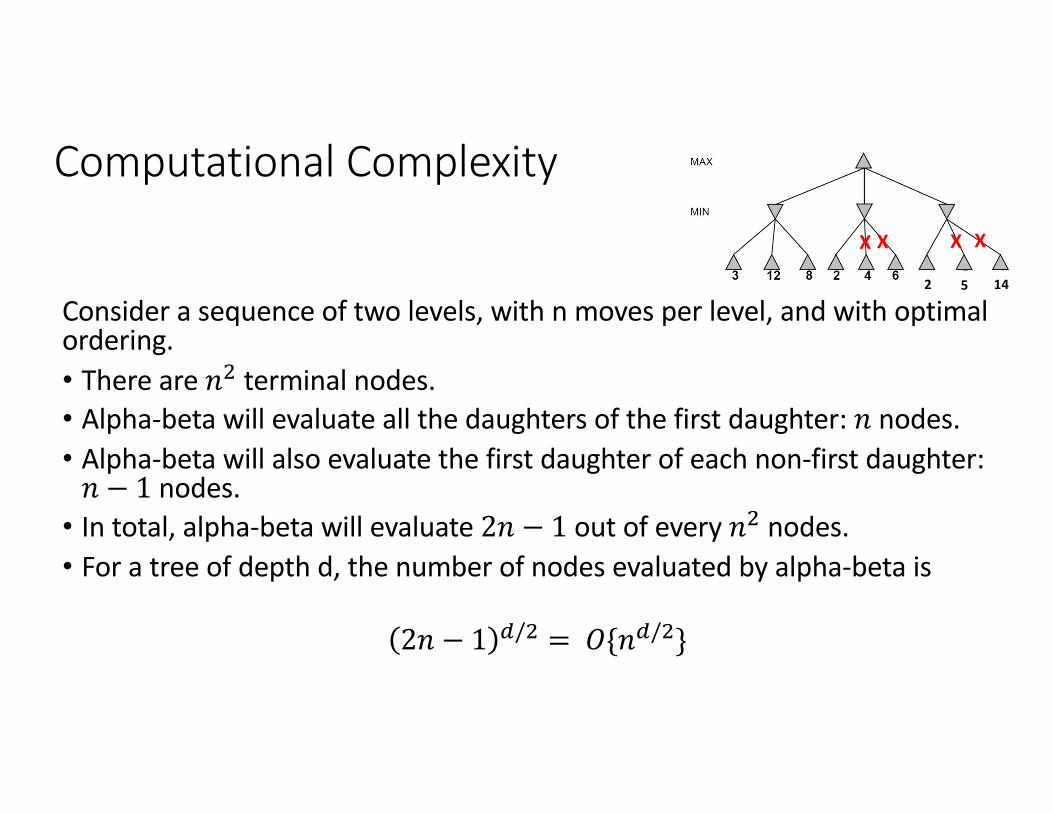
Computational Complexity
Consider a sequence of two levels, with n moves per level, and with optimal ordering. • There are 𝑛! terminal nodes.• Alpha-beta will evaluate all the daughters of the first daughter: 𝑛 nodes.• Alpha-beta will also evaluate the first daughter of each non-first daughter: 𝑛 − 1 nodes.• In total, alpha-beta will evaluate 2𝑛 − 1 out of every 𝑛! nodes.• For a tree of depth d, the number of nodes evaluated by alpha-beta is
2𝑛 − 1 "/! = 𝑂{𝑛"/!}
2 5 14
X X X X
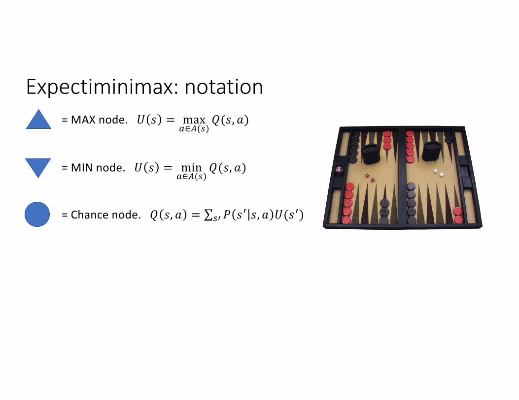
Expectiminimax: notation= MAX node. 𝑈 𝑠 = max
!∈#(%)𝑄(𝑠, 𝑎)
= MIN node. 𝑈 𝑠 = min!∈#(%)
𝑄(𝑠, 𝑎)
= Chance node. 𝑄 𝑠, 𝑎 = ∑%'𝑃 𝑠' 𝑠, 𝑎 𝑈(𝑠')
Outline: Exam 3 will be multiple-choice, on prairielearn, including 24 problems• 4 problems: Midterm 1 material• 4 problems: Midterm 2 material• 4-5 problems: minimax, alpha-beta, expectiminimax• 3-4 problems: game theory• 5-7 problems: MDP, reinforcement learning• 1 problem: AI fairness (definitions of fairness; causal graphs)• 1 problem: computer vision (similar triangles; convolution)
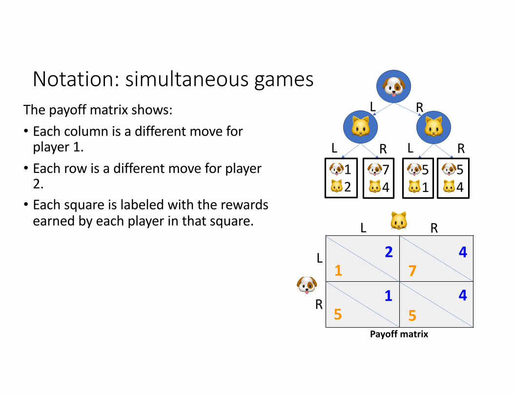
Notation: simultaneous gamesThe payoff matrix shows:• Each column is a different move for
player 1.• Each row is a different move for player
2.• Each square is labeled with the rewards
earned by each player in that square.
Payoff matrix
47
🐶
🐱 🐱
🐶1 🐱2
🐶7 🐱4
🐶5 🐱1
🐶5 🐱4
L
L L RR
R
45
15
21
L R
L
R
🐱
🐶
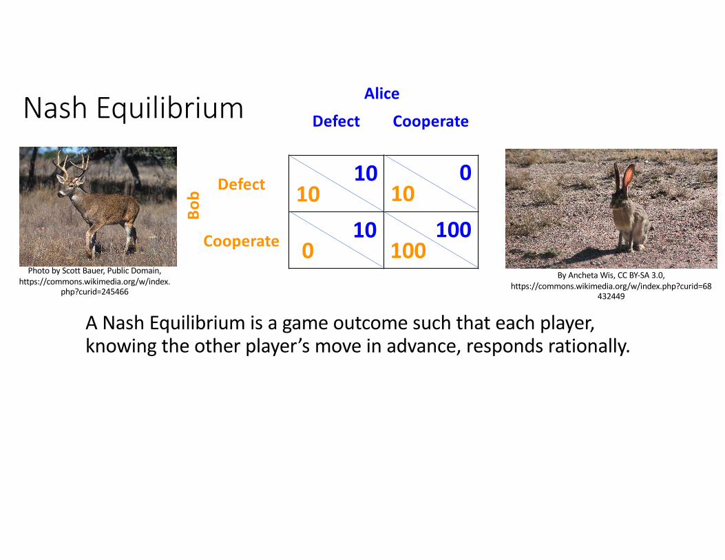
Nash Equilibrium
A Nash Equilibrium is a game outcome such that each player, knowing the other player’s move in advance, responds rationally.
Defect Cooperate
Defect
Cooperate
10
0 100
10010
10 100Photo by Scott Bauer, Public Domain,
https://commons.wikimedia.org/w/index.php?curid=245466
By Ancheta Wis, CC BY-SA 3.0, https://commons.wikimedia.org/w/index.php?curid=68
432449
Bob
Alice
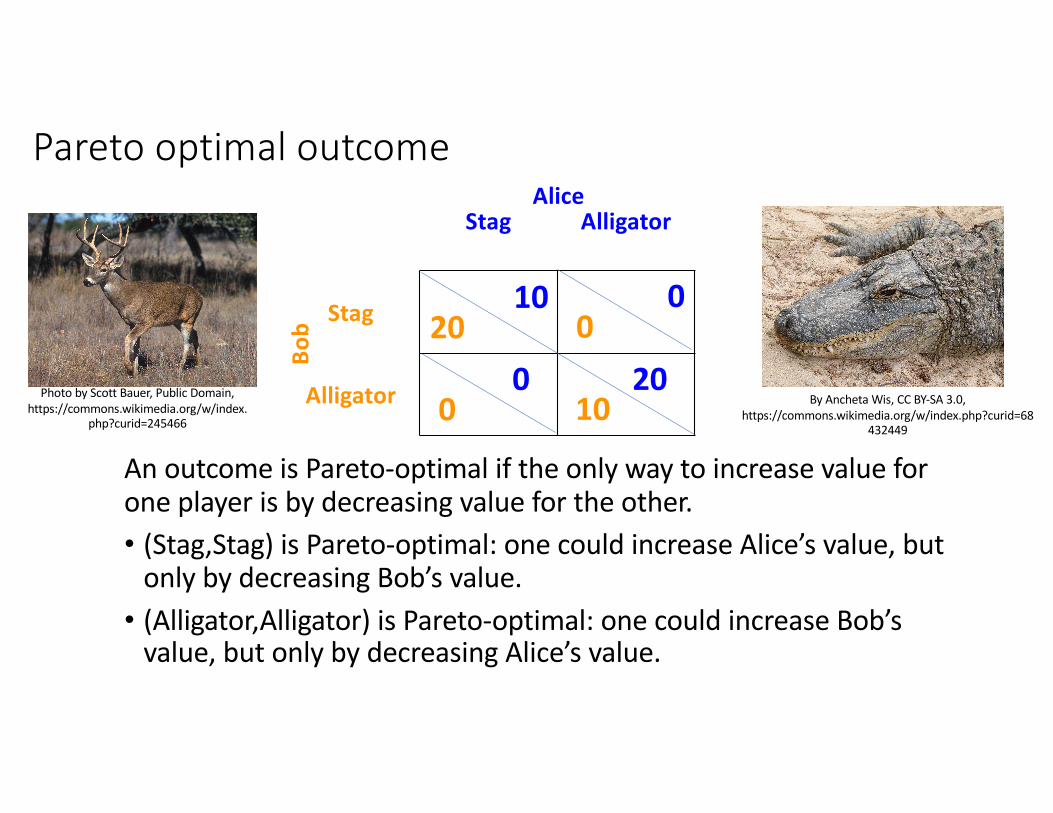
Pareto optimal outcome
An outcome is Pareto-optimal if the only way to increase value for one player is by decreasing value for the other.• (Stag,Stag) is Pareto-optimal: one could increase Alice’s value, but
only by decreasing Bob’s value.• (Alligator,Alligator) is Pareto-optimal: one could increase Bob’s
value, but only by decreasing Alice’s value.
Stag Alligator
Stag
Alligator
20
0 10
0010
0 20Photo by Scott Bauer, Public Domain, https://commons.wikimedia.org/w/index.
php?curid=245466
By Ancheta Wis, CC BY-SA 3.0, https://commons.wikimedia.org/w/index.php?curid=68
432449
Alice
Bob
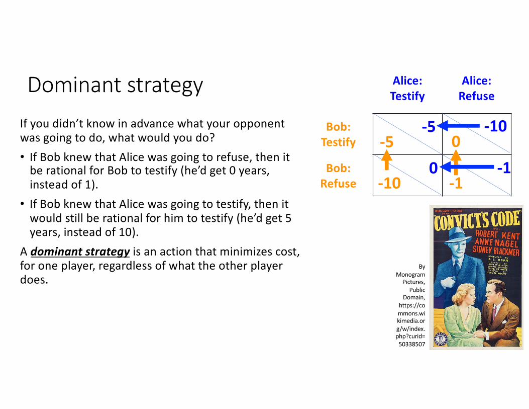
Dominant strategyIf you didn’t know in advance what your opponent was going to do, what would you do?• If Bob knew that Alice was going to refuse, then it
be rational for Bob to testify (he’d get 0 years, instead of 1).
• If Bob knew that Alice was going to testify, then it would still be rational for him to testify (he’d get 5 years, instead of 10).
A dominant strategy is an action that minimizes cost, for one player, regardless of what the other player does.
Alice:Testify
Alice:Refuse
Bob:Testify
Bob:Refuse
By Monogram
Pictures, Public
Domain, https://commons.wikimedia.org/w/index.php?curid=
50338507
-5
-10 -1
0-10-5
0 -1
Mixed-strategy Nash Equilibrium
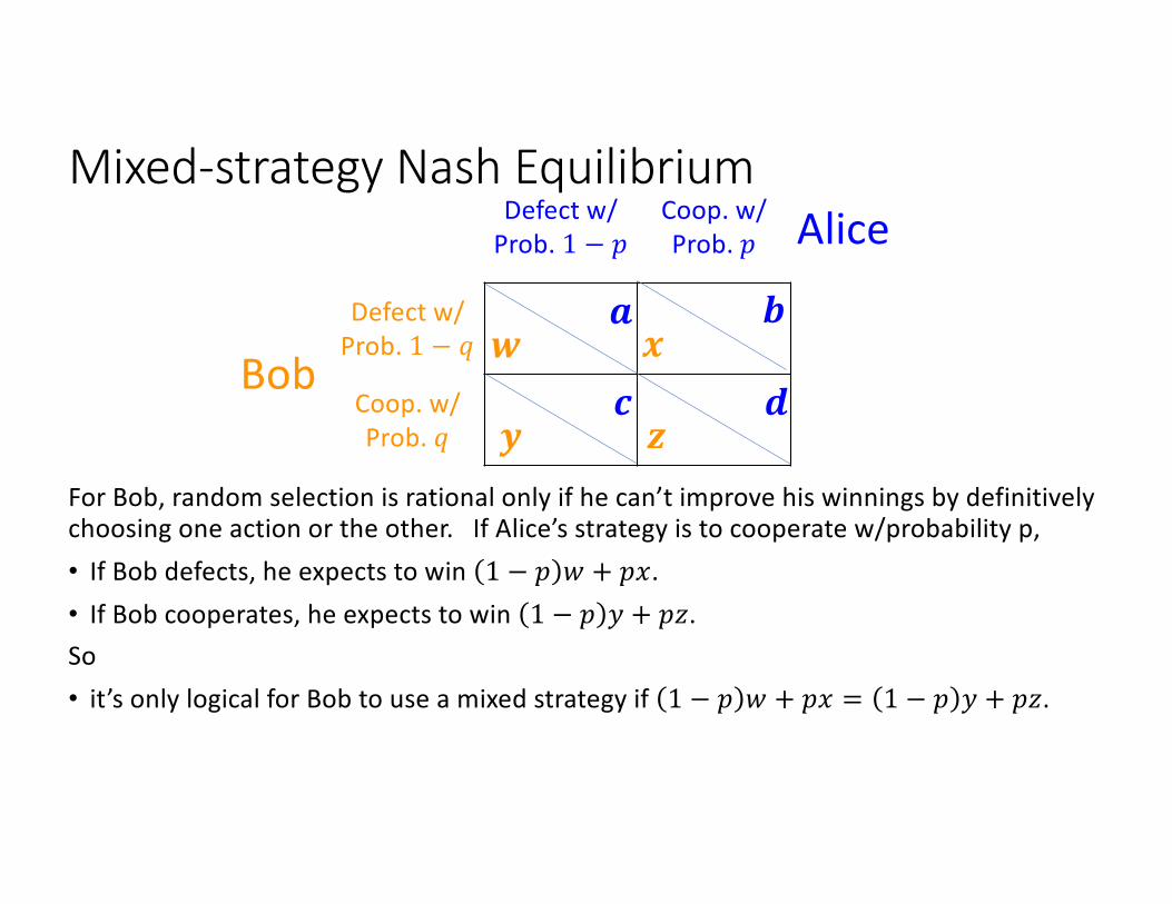
For Bob, random selection is rational only if he can’t improve his winnings by definitively choosing one action or the other. If Alice’s strategy is to cooperate w/probability p,• If Bob defects, he expects to win 1 − 𝑝 𝑤 + 𝑝𝑥.• If Bob cooperates, he expects to win 1 − 𝑝 𝑦 + 𝑝𝑧.So • it’s only logical for Bob to use a mixed strategy if 1 − 𝑝 𝑤 + 𝑝𝑥 = 1 − 𝑝 𝑦 + 𝑝𝑧.
Defect w/Prob. 1 − 𝑝
Coop. w/Prob. 𝑝
Defect w/Prob. 1 − 𝑞
Coop. w/Prob. 𝑞
𝒘
𝒚 𝒛
𝒙𝒃𝒂
𝒄 𝒅
Alice
Bob
Outline: Exam 3 will be multiple-choice, on prairielearn, including 24 problems• 4 problems: Midterm 1 material• 4 problems: Midterm 2 material• 4-5 problems: minimax, alpha-beta, expectiminimax• 3-4 problems: game theory• 5-7 problems: MDP, reinforcement learning• 1 problem: AI fairness (definitions of fairness; causal graphs)• 1 problem: computer vision (similar triangles; convolution)
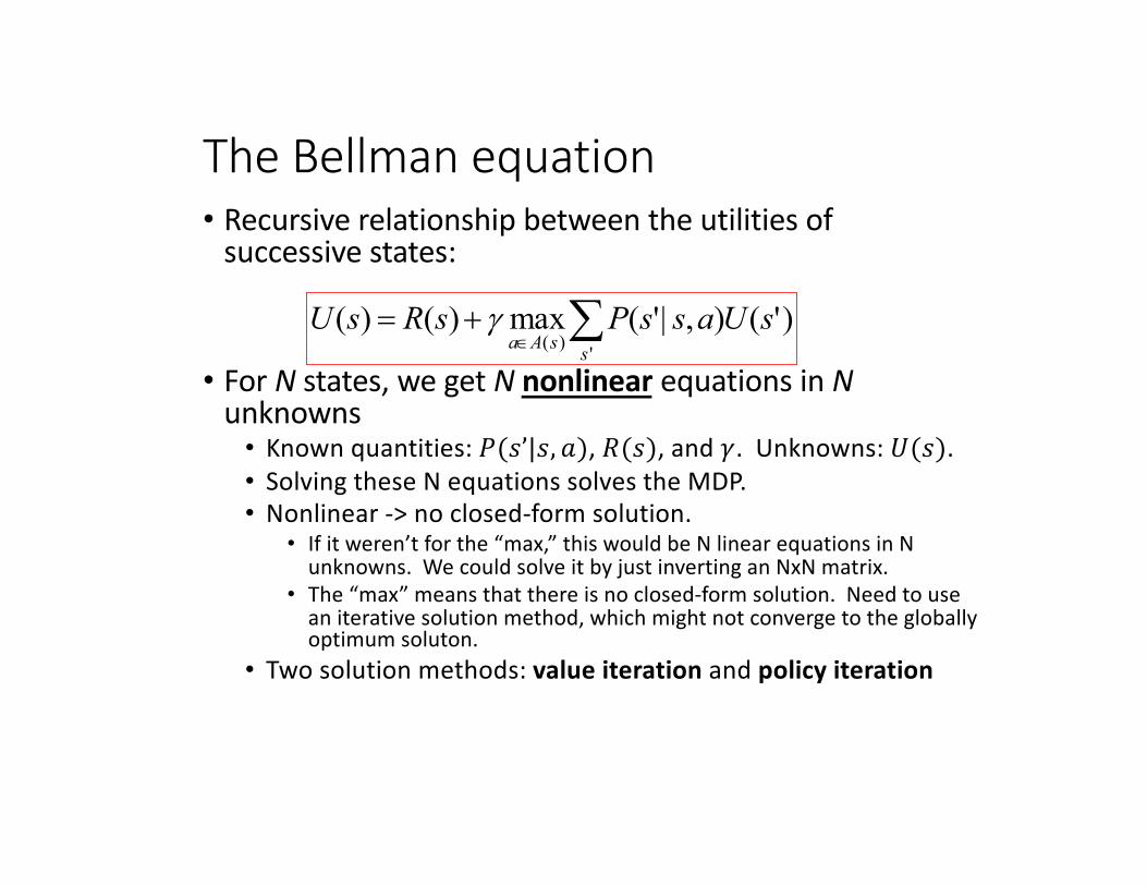
The Bellman equation• Recursive relationship between the utilities of
successive states:
• For N states, we get N nonlinear equations in Nunknowns• Known quantities: 𝑃(𝑠’|𝑠, 𝑎), 𝑅(𝑠), and 𝛾. Unknowns: 𝑈(𝑠).• Solving these N equations solves the MDP.• Nonlinear -> no closed-form solution.
• If it weren’t for the “max,” this would be N linear equations in N unknowns. We could solve it by just inverting an NxN matrix.
• The “max” means that there is no closed-form solution. Need to use an iterative solution method, which might not converge to the globally optimum soluton.
• Two solution methods: value iteration and policy iteration
åÎ
+=')(
)'(),|'(max)()(ssAa
sUassPsRsU g
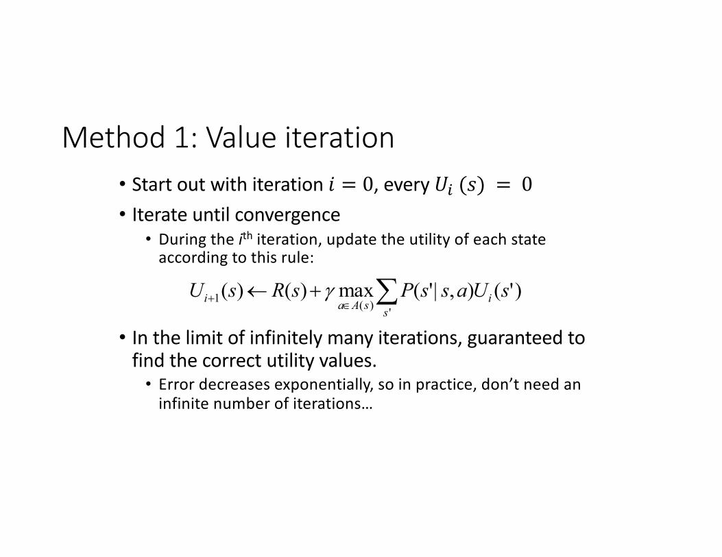
Method 1: Value iteration• Start out with iteration 𝑖 = 0, every 𝑈$ (𝑠) = 0• Iterate until convergence
• During the ith iteration, update the utility of each state according to this rule:
• In the limit of infinitely many iterations, guaranteed to find the correct utility values.• Error decreases exponentially, so in practice, don’t need an
infinite number of iterations…
åÎ+ +¬
')(1 )'(),|'(max)()(s
isAai sUassPsRsU g
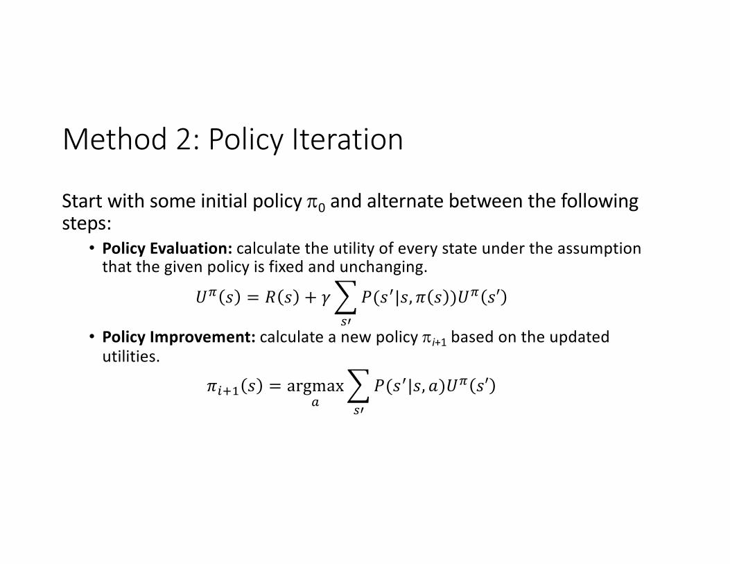
Method 2: Policy Iteration
Start with some initial policy p0 and alternate between the following steps:
• Policy Evaluation: calculate the utility of every state under the assumption that the given policy is fixed and unchanging.
𝑈( 𝑠 = 𝑅 𝑠 + 𝛾=%'
𝑃(𝑠'|𝑠, 𝜋 𝑠 )𝑈( 𝑠′
• Policy Improvement: calculate a new policy pi+1 based on the updated utilities.
𝜋)*+ 𝑠 = argmax!
=%'
𝑃(𝑠'|𝑠, 𝑎)𝑈( 𝑠′
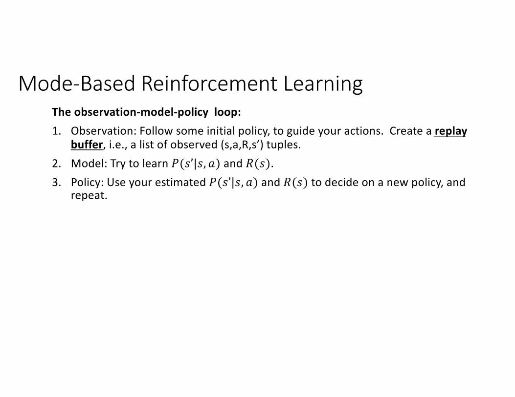
Mode-Based Reinforcement LearningThe observation-model-policy loop: 1. Observation: Follow some initial policy, to guide your actions. Create a replay
buffer, i.e., a list of observed (s,a,R,s’) tuples.2. Model: Try to learn 𝑃(𝑠’|𝑠, 𝑎) and 𝑅(𝑠).3. Policy: Use your estimated 𝑃(𝑠’|𝑠, 𝑎) and 𝑅(𝑠) to decide on a new policy, and
repeat.
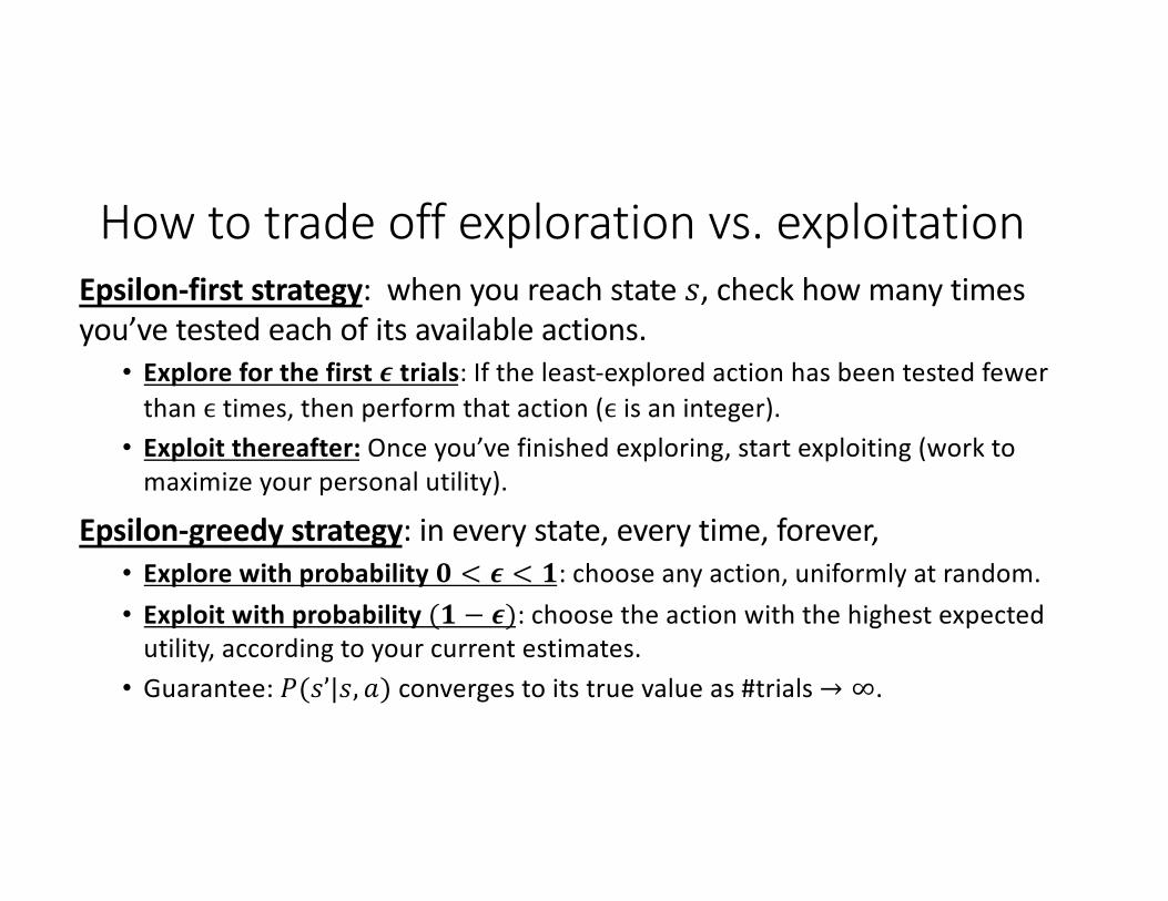
How to trade off exploration vs. exploitationEpsilon-first strategy: when you reach state 𝑠, check how many times you’ve tested each of its available actions.
• Explore for the first 𝝐 trials: If the least-explored action has been tested fewer than ϵ times, then perform that action (ϵ is an integer).
• Exploit thereafter: Once you’ve finished exploring, start exploiting (work to maximize your personal utility).
Epsilon-greedy strategy: in every state, every time, forever,• Explore with probability 𝟎 < 𝝐 < 𝟏: choose any action, uniformly at random.• Exploit with probability (𝟏 − 𝝐): choose the action with the highest expected
utility, according to your current estimates.• Guarantee: 𝑃(𝑠’|𝑠, 𝑎) converges to its true value as #trials → ∞.
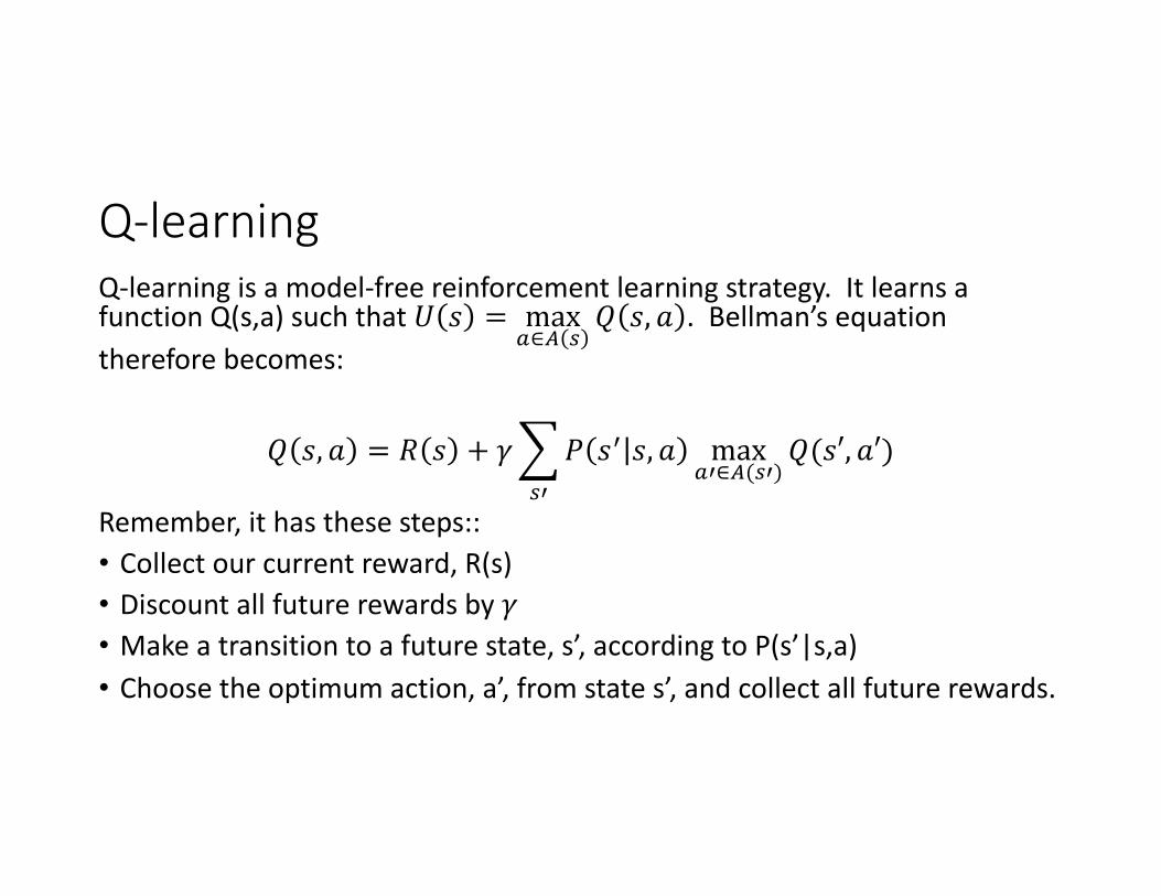
Q-learningQ-learning is a model-free reinforcement learning strategy. It learns a function Q(s,a) such that 𝑈 𝑠 = max
!∈# $𝑄 𝑠, 𝑎 . Bellman’s equation
therefore becomes:
𝑄 𝑠, 𝑎 = 𝑅 𝑠 + 𝛾-$%
𝑃 𝑠% 𝑠, 𝑎 max!%∈#($%)
𝑄(𝑠′, 𝑎′)
Remember, it has these steps::• Collect our current reward, R(s)• Discount all future rewards by 𝛾• Make a transition to a future state, s’, according to P(s’|s,a)• Choose the optimum action, a’, from state s’, and collect all future rewards.
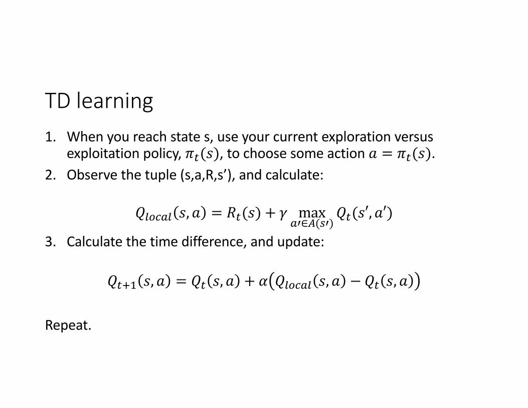
TD learning1. When you reach state s, use your current exploration versus
exploitation policy, 𝜋%(𝑠), to choose some action 𝑎 = 𝜋%(𝑠). 2. Observe the tuple (s,a,R,s’), and calculate:
𝑄&'()& 𝑠, 𝑎 = 𝑅%(𝑠) + 𝛾 max)*∈,(.*)
𝑄%(𝑠′, 𝑎′)
3. Calculate the time difference, and update:
𝑄%01 𝑠, 𝑎 = 𝑄% 𝑠, 𝑎 + 𝛼 𝑄&'()& 𝑠, 𝑎 − 𝑄% 𝑠, 𝑎
Repeat.
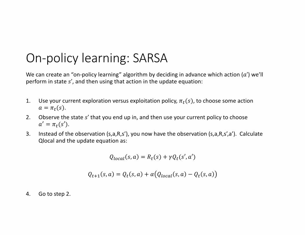
On-policy learning: SARSAWe can create an “on-policy learning” algorithm by deciding in advance which action (𝑎’) we’ll perform in state 𝑠’, and then using that action in the update equation:
1. Use your current exploration versus exploitation policy, 𝜋!(𝑠), to choose some action 𝑎 = 𝜋!(𝑠).
2. Observe the state 𝑠’ that you end up in, and then use your current policy to choose 𝑎" = 𝜋!(𝑠′).
3. Instead of the observation (s,a,R,s’), you now have the observation (s,a,R,s’,a’). Calculate Qlocal and the update equation as:
𝑄#$%&# 𝑠, 𝑎 = 𝑅!(𝑠) + 𝛾𝑄!(𝑠′, 𝑎′)
𝑄!'( 𝑠, 𝑎 = 𝑄! 𝑠, 𝑎 + 𝛼 𝑄#$%&# 𝑠, 𝑎 − 𝑄! 𝑠, 𝑎
4. Go to step 2.
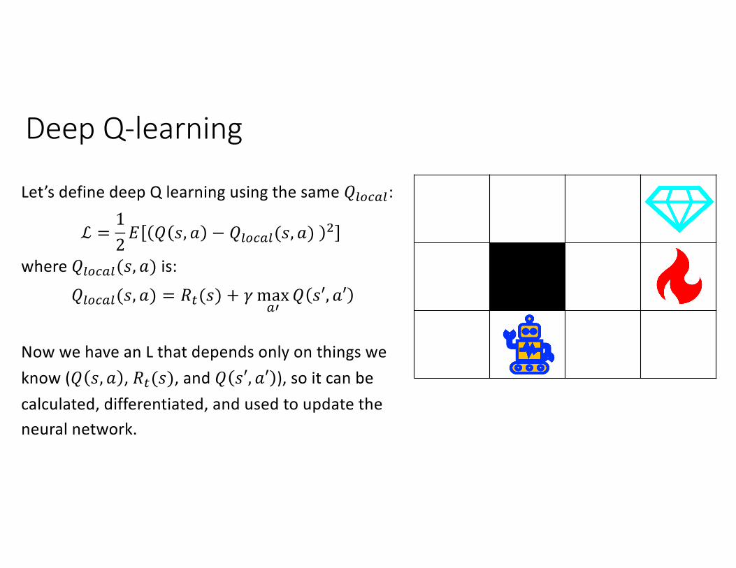
Deep Q-learning
Let’s define deep Q learning using the same 𝑄,-.!,:
ℒ =12𝐸 𝑄 𝑠, 𝑎 − 𝑄,-.!,(𝑠, 𝑎) /
where 𝑄,-.!,(𝑠, 𝑎) is:
𝑄,-.!,(𝑠, 𝑎) = 𝑅0(𝑠) + 𝛾 max!'
𝑄 𝑠′, 𝑎′
Now we have an L that depends only on things we know (𝑄 𝑠, 𝑎 , 𝑅0(𝑠), and 𝑄 𝑠′, 𝑎′ ), so it can be calculated, differentiated, and used to update the neural network.
Policy learning methods• Suppose that 𝑠 is continuous, but 𝑎 is discrete (e.g., a one-hot vector).• Then learning the policy directly can be much faster than learning Q
values.• We can train a neural network for a stochastic policy---a policy that
chooses an action at random, using the probability distribution:
𝜋 𝑠, 𝑎 =𝑒2(.,))
∑)* 𝑒2(.,)*)
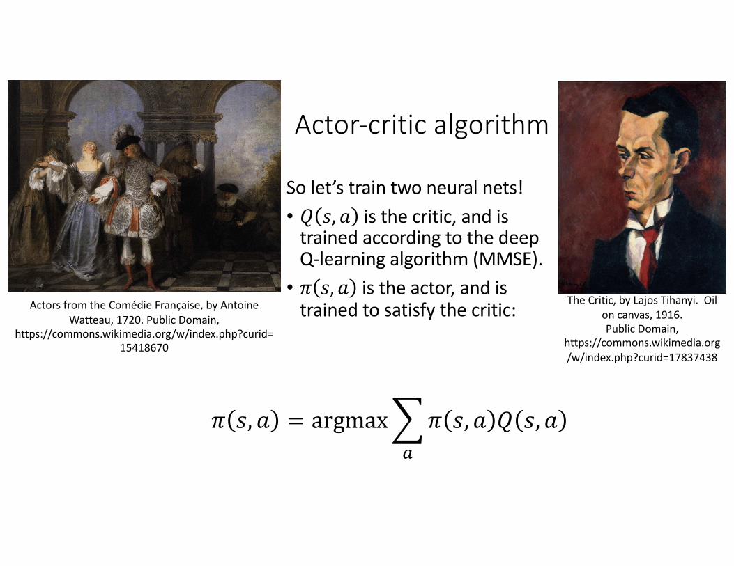
Actor-critic algorithm
So let’s train two neural nets!• 𝑄 𝑠, 𝑎 is the critic, and is
trained according to the deep Q-learning algorithm (MMSE). • 𝜋 𝑠, 𝑎 is the actor, and is
trained to satisfy the critic: The Critic, by Lajos Tihanyi. Oil on canvas, 1916.Public Domain,
https://commons.wikimedia.org/w/index.php?curid=17837438
Actors from the Comédie Française, by Antoine Watteau, 1720. Public Domain,
https://commons.wikimedia.org/w/index.php?curid=15418670
𝜋 𝑠, 𝑎 = argmax3L
𝜋 𝑠, 𝑎 𝑄 𝑠, 𝑎
Outline: Exam 3 will be multiple-choice, on prairielearn, including 24 problems• 4 problems: Midterm 1 material• 4 problems: Midterm 2 material• 4-5 problems: minimax, alpha-beta, expectiminimax• 3-4 problems: game theory• 5-7 problems: MDP, reinforcement learning• 1 problem: AI fairness (definitions of fairness; causal graphs)• 1 problem: computer vision (similar triangles; convolution)
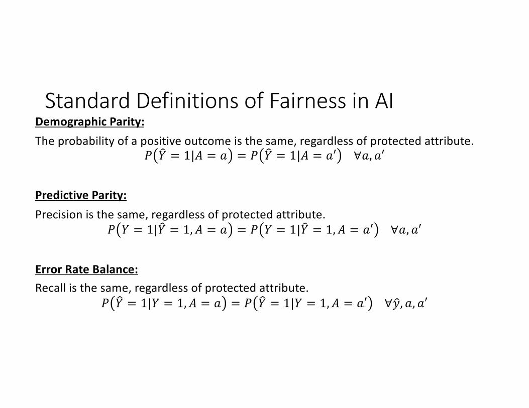
Standard Definitions of Fairness in AIDemographic Parity:The probability of a positive outcome is the same, regardless of protected attribute.
𝑃 M𝑌 = 1|𝐴 = 𝑎 = 𝑃 M𝑌 = 1|𝐴 = 𝑎′ ∀𝑎, 𝑎′
Predictive Parity:Precision is the same, regardless of protected attribute.
𝑃 𝑌 = 1| M𝑌 = 1, 𝐴 = 𝑎 = 𝑃 𝑌 = 1| M𝑌 = 1, 𝐴 = 𝑎′ ∀𝑎, 𝑎′
Error Rate Balance:Recall is the same, regardless of protected attribute.
𝑃 M𝑌 = 1|𝑌 = 1, 𝐴 = 𝑎 = 𝑃 M𝑌 = 1|𝑌 = 1, 𝐴 = 𝑎′ ∀ Q𝑦, 𝑎, 𝑎′
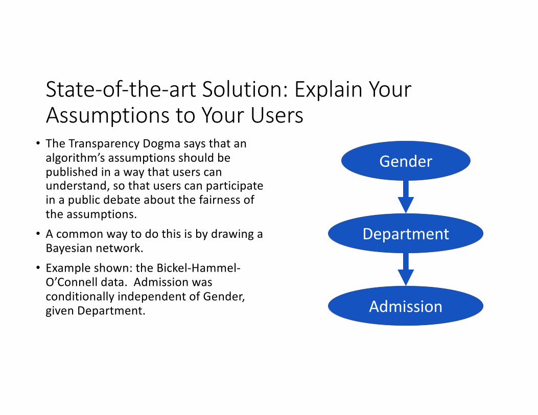
State-of-the-art Solution: Explain Your Assumptions to Your Users
• The Transparency Dogma says that an algorithm’s assumptions should be published in a way that users can understand, so that users can participate in a public debate about the fairness of the assumptions.
• A common way to do this is by drawing a Bayesian network.
• Example shown: the Bickel-Hammel-O’Connell data. Admission was conditionally independent of Gender, given Department.
Gender
Department
Admission
Outline: Exam 3 will be multiple-choice, on prairielearn, including 24 problems• 4 problems: Midterm 1 material• 4 problems: Midterm 2 material• 4-5 problems: minimax, alpha-beta, expectiminimax• 3-4 problems: game theory• 5-7 problems: MDP, reinforcement learning• 1 problem: AI fairness (definitions of fairness; causal graphs)• 1 problem: computer vision (similar triangles; convolution)
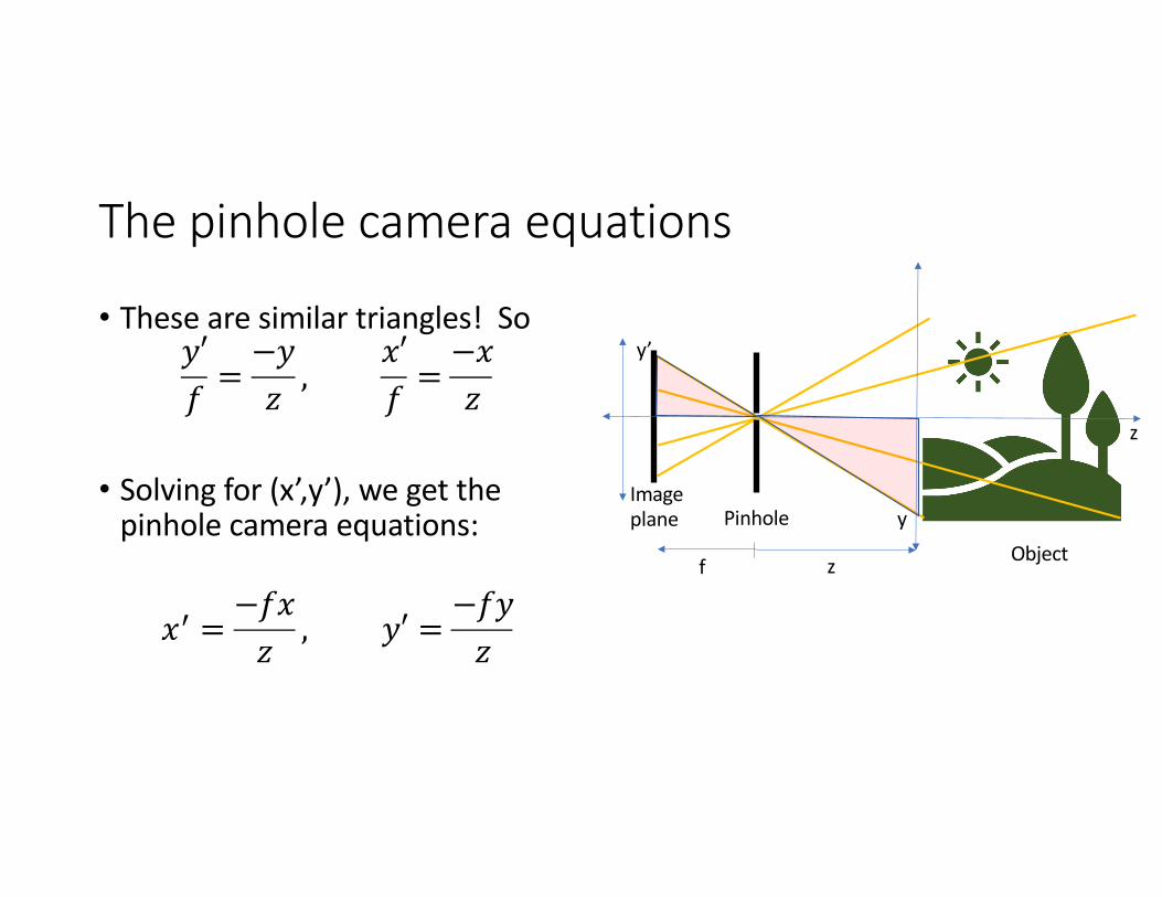
The pinhole camera equations
• These are similar triangles! So𝑦′𝑓 =
−𝑦𝑧 ,
𝑥′𝑓 =
−𝑥𝑧
• Solving for (x’,y’), we get the pinhole camera equations:
𝑥* =−𝑓𝑥𝑧
, 𝑦′ =−𝑓𝑦𝑧
Imageplane
Object
Pinhole
y’
y
z
f z
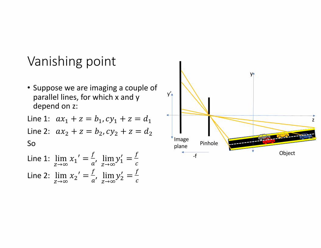
Vanishing point
• Suppose we are imaging a couple of parallel lines, for which x and y depend on z:
Line 1: 𝑎𝑥( + 𝑧 = 𝑏(, 𝑐𝑦( + 𝑧 = 𝑑(Line 2: 𝑎𝑥) + 𝑧 = 𝑏), 𝑐𝑦) + 𝑧 = 𝑑)So
Line 1: lim*→,
𝑥(′ =-!
, lim*→,
𝑦(% =-.
Line 2: lim*→,
𝑥)′ =-!
, lim*→,
𝑦)% =-.
Imageplane
Object
Pinhole
y’
y
z
-f
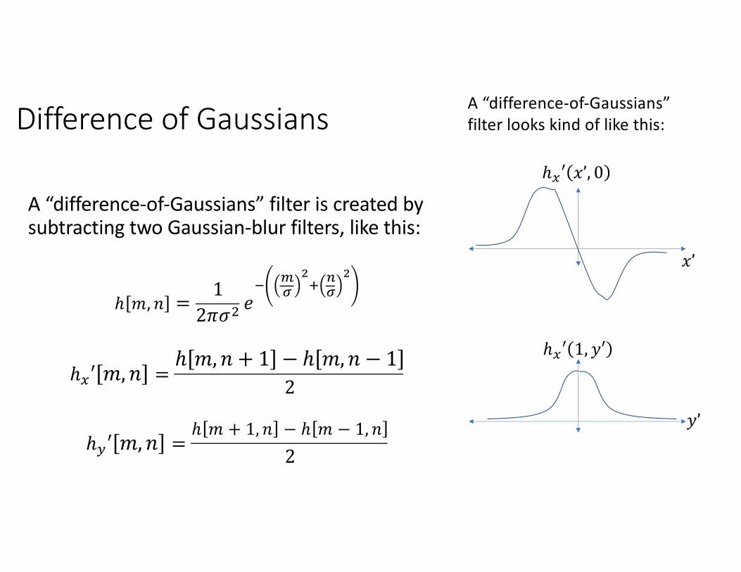
Difference of Gaussians
A “difference-of-Gaussians” filter is created by subtracting two Gaussian-blur filters, like this:
ℎ 𝑚, 𝑛 =1
2𝜋𝜎) 𝑒/ 0
1!2 31
!
ℎ4′ 𝑚,𝑛 =ℎ 𝑚, 𝑛 + 1 − ℎ 𝑚, 𝑛 − 1
2
ℎ5′ 𝑚,𝑛 =ℎ 𝑚 + 1, 𝑛 − ℎ 𝑚 − 1, 𝑛
2
𝑥’
ℎ1′ 𝑥’, 0
A “difference-of-Gaussians” filter looks kind of like this:
𝑦’
ℎ1′ 1, 𝑦′
Some Sample Problems
• Review exam Question 3: Alpha-beta pruning• Review exam Question 10: Game theory• Review exam Question 14: MDP
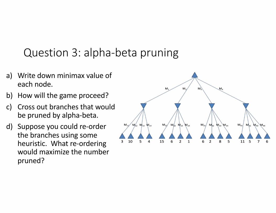
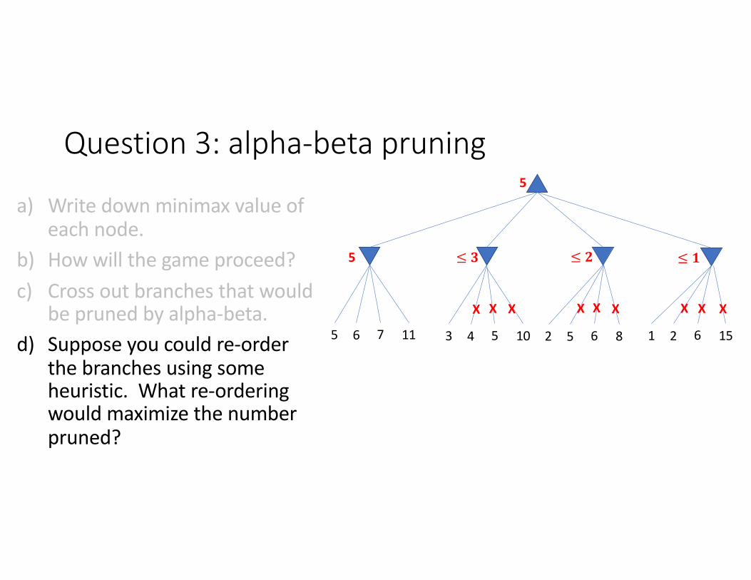
Question 3: alpha-beta pruning
a) Write down minimax value of each node.
b) How will the game proceed?c) Cross out branches that would
be pruned by alpha-beta.d) Suppose you could re-order
the branches using some heuristic. What re-ordering would maximize the number pruned?
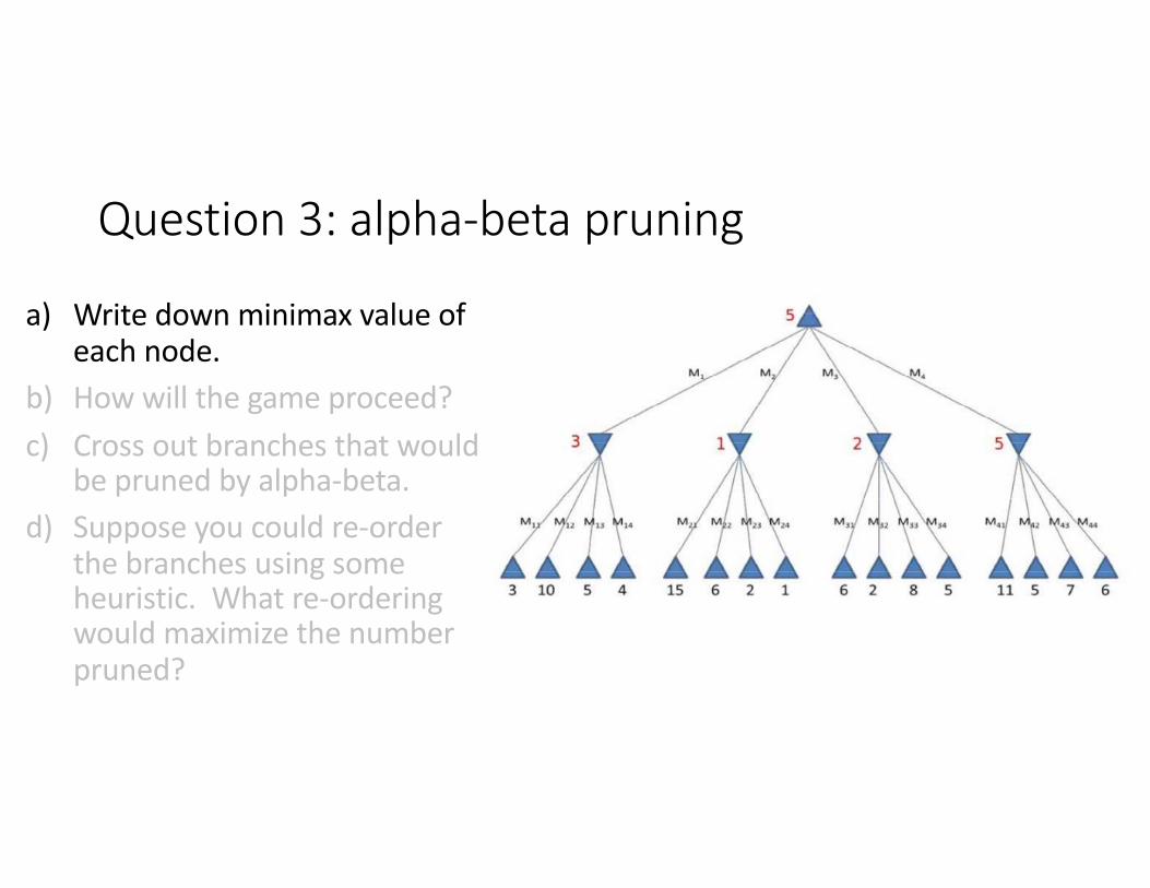
Question 3: alpha-beta pruning
a) Write down minimax value of each node.
b) How will the game proceed?c) Cross out branches that would
be pruned by alpha-beta.d) Suppose you could re-order
the branches using some heuristic. What re-ordering would maximize the number pruned?
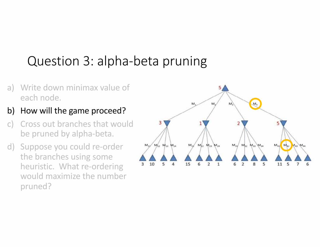
Question 3: alpha-beta pruning
a) Write down minimax value of each node.
b) How will the game proceed?c) Cross out branches that would
be pruned by alpha-beta.d) Suppose you could re-order
the branches using some heuristic. What re-ordering would maximize the number pruned?
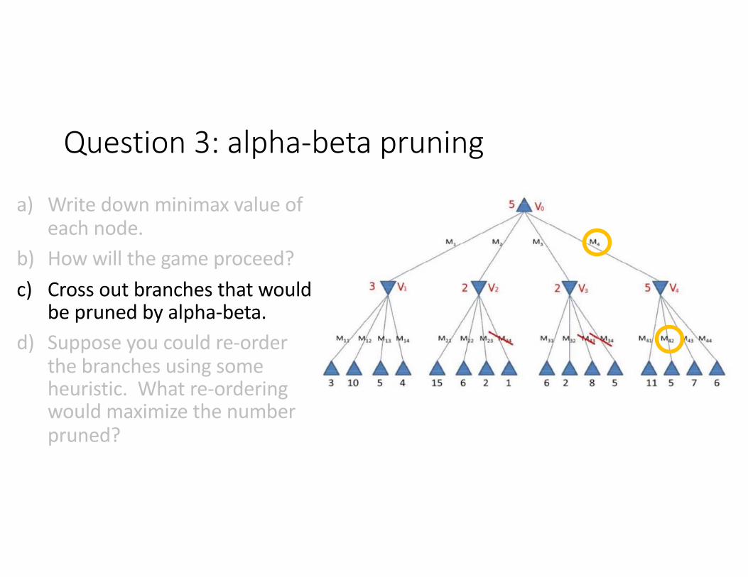
Question 3: alpha-beta pruning
a) Write down minimax value of each node.
b) How will the game proceed?c) Cross out branches that would
be pruned by alpha-beta.d) Suppose you could re-order
the branches using some heuristic. What re-ordering would maximize the number pruned?
Question 3: alpha-beta pruning
a) Write down minimax value of each node.
b) How will the game proceed?c) Cross out branches that would
be pruned by alpha-beta.d) Suppose you could re-order
the branches using some heuristic. What re-ordering would maximize the number pruned?
5 6 7 11 3 4 5 10 2 5 6 8 1 2 6 15
5 ≤ 𝟑 ≤ 𝟐 ≤ 𝟏
5
X X X X X X X X X
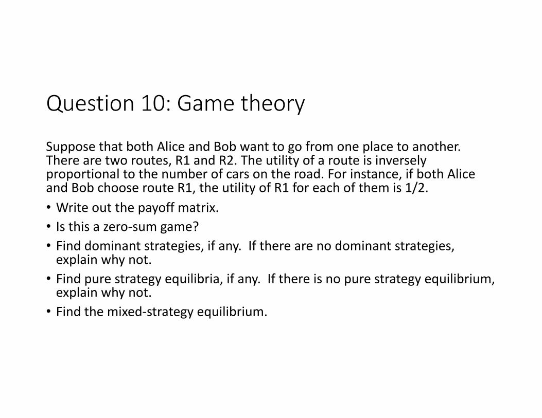
Question 10: Game theory
Suppose that both Alice and Bob want to go from one place to another. There are two routes, R1 and R2. The utility of a route is inversely proportional to the number of cars on the road. For instance, if both Alice and Bob choose route R1, the utility of R1 for each of them is 1/2.• Write out the payoff matrix.• Is this a zero-sum game?• Find dominant strategies, if any. If there are no dominant strategies,
explain why not.• Find pure strategy equilibria, if any. If there is no pure strategy equilibrium,
explain why not.• Find the mixed-strategy equilibrium.
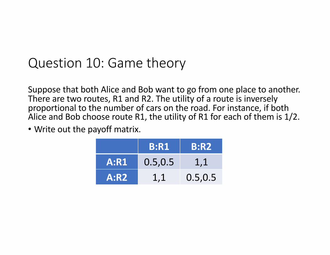
Question 10: Game theory
Suppose that both Alice and Bob want to go from one place to another. There are two routes, R1 and R2. The utility of a route is inversely proportional to the number of cars on the road. For instance, if both Alice and Bob choose route R1, the utility of R1 for each of them is 1/2.• Write out the payoff matrix.
B:R1 B:R2A:R1 0.5,0.5 1,1A:R2 1,1 0.5,0.5
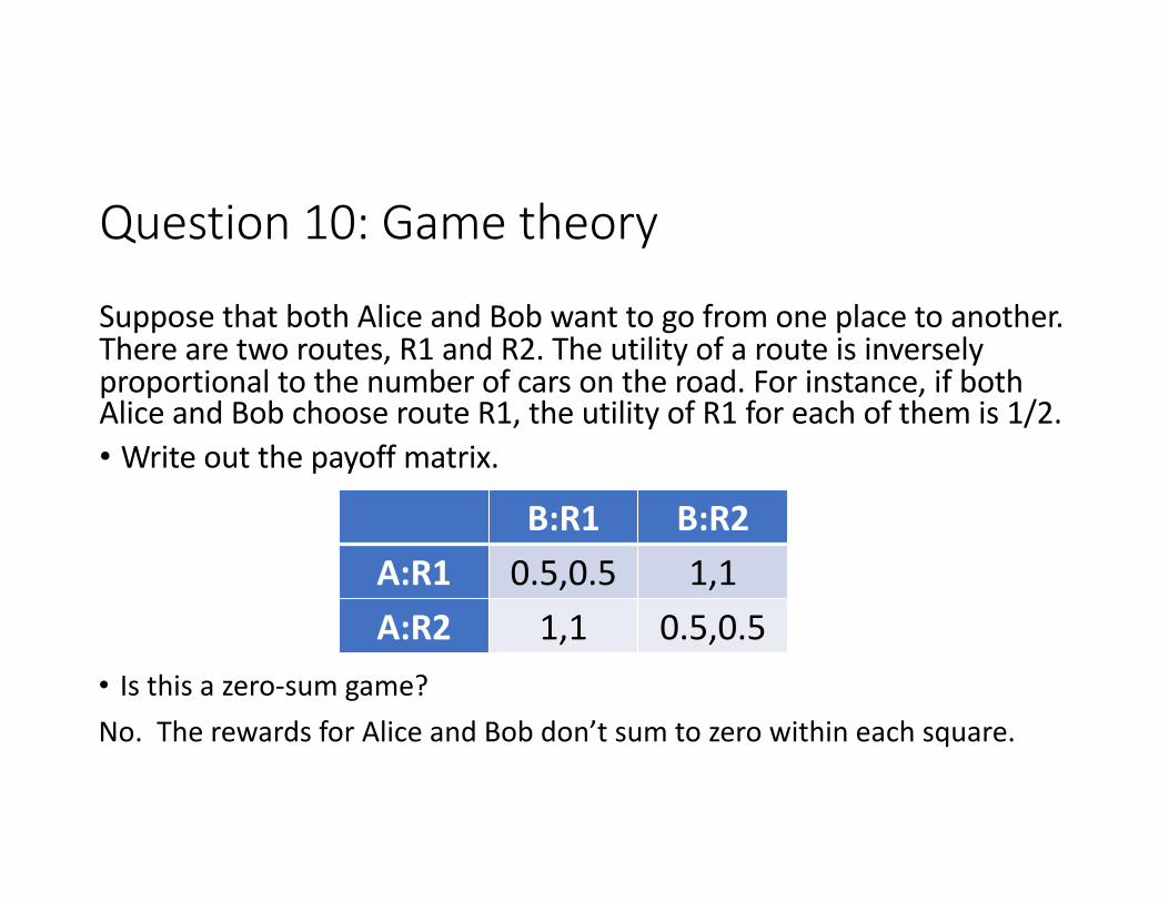
• Is this a zero-sum game?No. The rewards for Alice and Bob don’t sum to zero within each square.
Question 10: Game theory
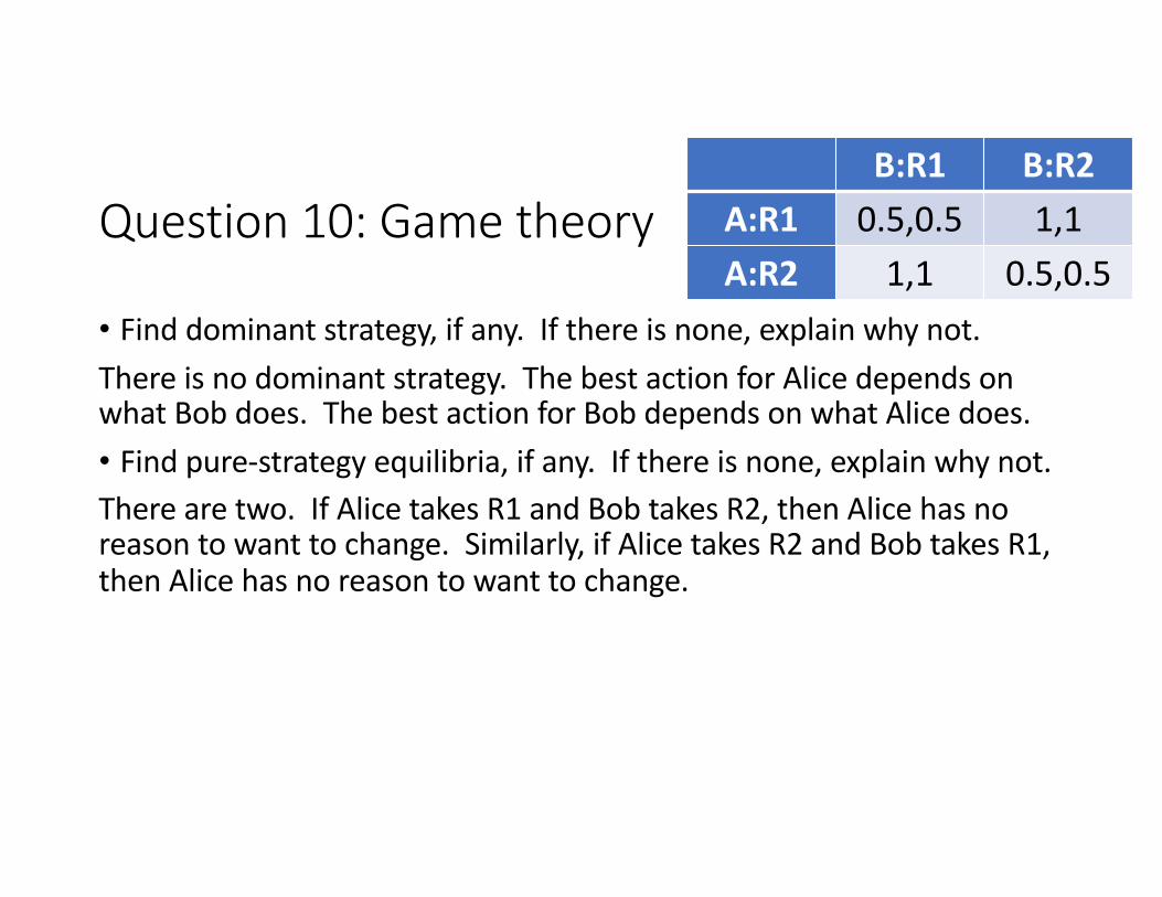
• Find dominant strategy, if any. If there is none, explain why not.There is no dominant strategy. The best action for Alice depends on what Bob does. The best action for Bob depends on what Alice does.• Find pure-strategy equilibria, if any. If there is none, explain why not.There are two. If Alice takes R1 and Bob takes R2, then Alice has no reason to want to change. Similarly, if Alice takes R2 and Bob takes R1, then Alice has no reason to want to change.
B:R1 B:R2A:R1 0.5,0.5 1,1A:R2 1,1 0.5,0.5
Question 10: Game theory
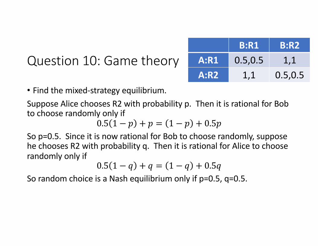
• Find the mixed-strategy equilibrium.Suppose Alice chooses R2 with probability p. Then it is rational for Bob to choose randomly only if
0.5 1 − 𝑝 + 𝑝 = 1 − 𝑝 + 0.5𝑝So p=0.5. Since it is now rational for Bob to choose randomly, suppose he chooses R2 with probability q. Then it is rational for Alice to choose randomly only if
0.5 1 − 𝑞 + 𝑞 = 1 − 𝑞 + 0.5𝑞So random choice is a Nash equilibrium only if p=0.5, q=0.5.
B:R1 B:R2A:R1 0.5,0.5 1,1A:R2 1,1 0.5,0.5
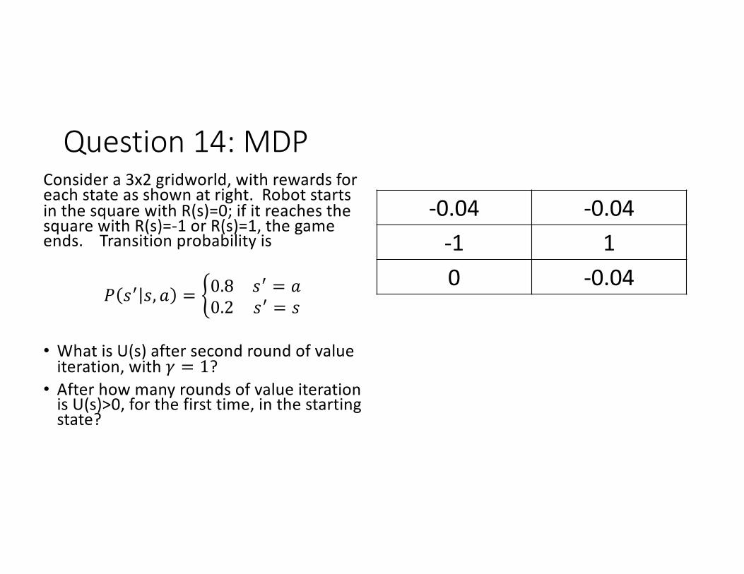
Question 14: MDPConsider a 3x2 gridworld, with rewards for each state as shown at right. Robot starts in the square with R(s)=0; if it reaches the square with R(s)=-1 or R(s)=1, the game ends. Transition probability is
𝑃 𝑠' 𝑠, 𝑎 = V0.8 𝑠' = 𝑎0.2 𝑠' = 𝑠
• What is U(s) after second round of value iteration, with 𝛾 = 1?
• After how many rounds of value iteration is U(s)>0, for the first time, in the starting state?
-0.04 -0.04-1 10 -0.04
Question 14: MDP
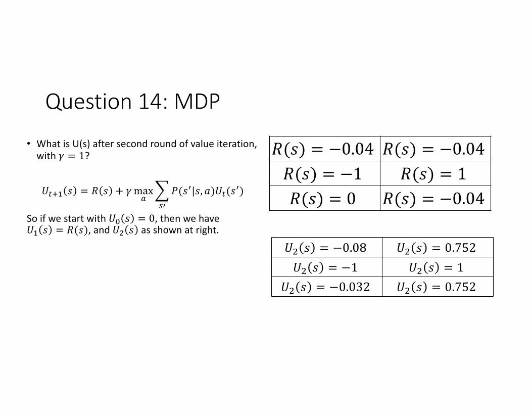
• What is U(s) after second round of value iteration, with 𝛾 = 1?
𝑈!'( 𝑠 = 𝑅 𝑠 + 𝛾max&
5)"
𝑃(𝑠"|𝑠, 𝑎)𝑈!(𝑠")
So if we start with 𝑈* 𝑠 = 0, then we have 𝑈( 𝑠 = 𝑅(𝑠), and 𝑈+ 𝑠 as shown at right.
𝑅(𝑠) = −0.04 𝑅(𝑠) = −0.04𝑅(𝑠) = −1 𝑅(𝑠) = 1𝑅(𝑠) = 0 𝑅(𝑠) = −0.04
𝑈/ 𝑠 = −0.08 𝑈/ 𝑠 = 0.752𝑈/ 𝑠 = −1 𝑈/ 𝑠 = 1
𝑈/ 𝑠 = −0.032 𝑈/ 𝑠 = 0.752
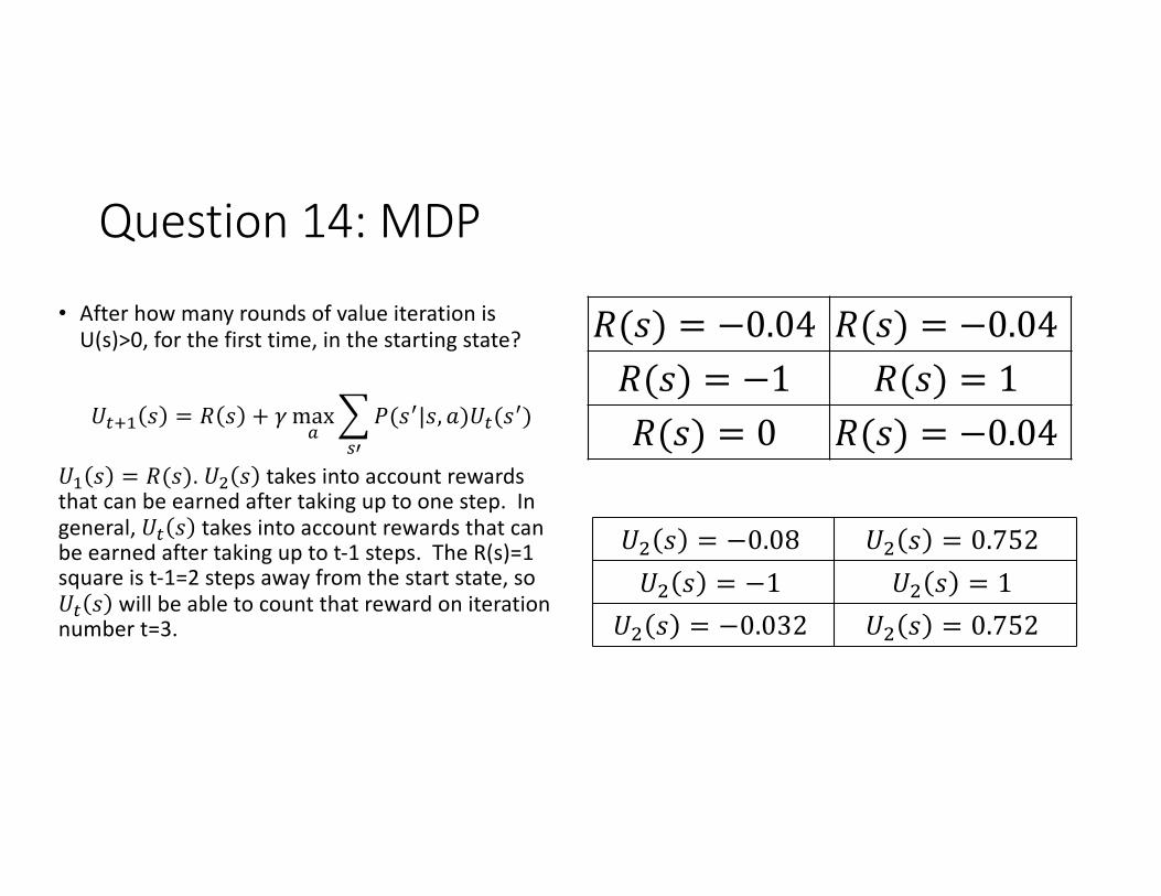
Question 14: MDP
• After how many rounds of value iteration is U(s)>0, for the first time, in the starting state?
𝑈!'( 𝑠 = 𝑅 𝑠 + 𝛾max&
5)"
𝑃(𝑠"|𝑠, 𝑎)𝑈!(𝑠")
𝑈( 𝑠 = 𝑅(𝑠). 𝑈+ 𝑠 takes into account rewards that can be earned after taking up to one step. In general, 𝑈! 𝑠 takes into account rewards that can be earned after taking up to t-1 steps. The R(s)=1 square is t-1=2 steps away from the start state, so 𝑈! 𝑠 will be able to count that reward on iteration number t=3.
𝑅(𝑠) = −0.04 𝑅(𝑠) = −0.04𝑅(𝑠) = −1 𝑅(𝑠) = 1𝑅(𝑠) = 0 𝑅(𝑠) = −0.04
𝑈/ 𝑠 = −0.08 𝑈/ 𝑠 = 0.752𝑈/ 𝑠 = −1 𝑈/ 𝑠 = 1
𝑈/ 𝑠 = −0.032 𝑈/ 𝑠 = 0.752

Outline: Exam 3 will be multiple-choice, on prairielearn, including 24 problems• 4 problems: Midterm 1 material• 4 problems: Midterm 2 material• 4-5 problems: minimax, alpha-beta, expectiminimax• 3-4 problems: game theory• 5-7 problems: MDP, reinforcement learning• 1 problem: AI fairness (definitions of fairness; causal graphs)• 1 problem: computer vision (similar triangles; convolution)