Lecture 22

Adjunct Methods

Part 1

Motivation

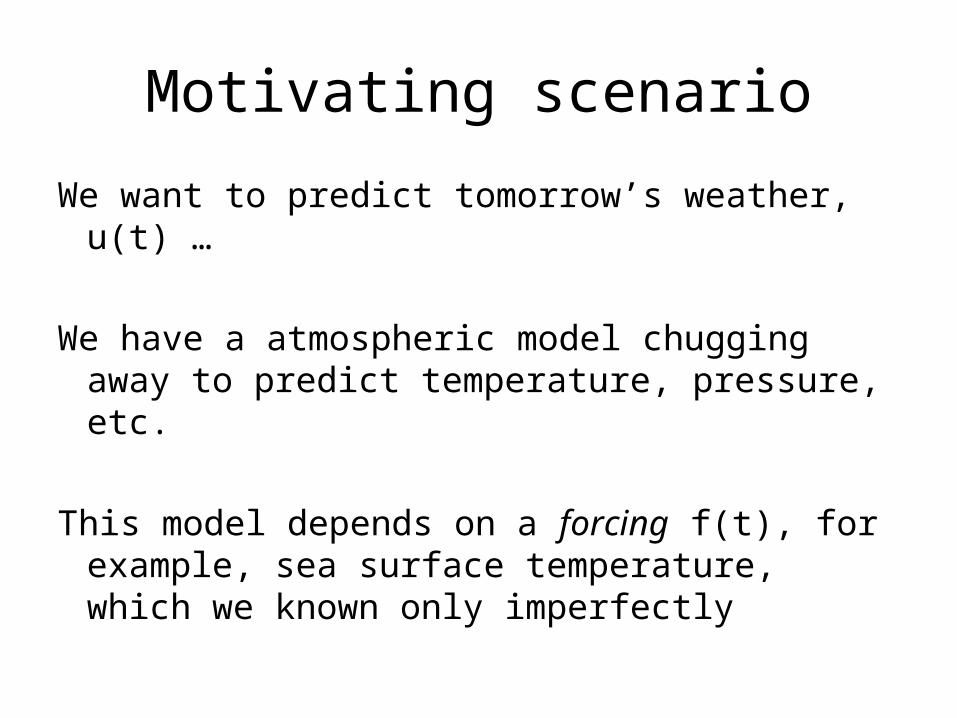
Motivating scenario

We want to predict tomorrow’s weather, u(t) …

We have a atmospheric model chugging away to predict temperature, pressure, etc.

This model depends on a forcing f(t), for example, sea surface temperature, which we known only imperfectly

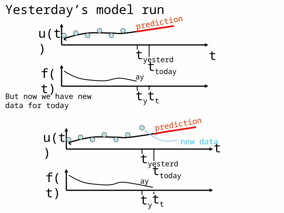
Yesterday’s model run

t

u(t)

tyesterday

f(t)

ty

prediction

ttoday

But now we have newdata for today

tu(t)

tyesterday

f(t)

ty

prediction

ttoday

tt

tt

new data

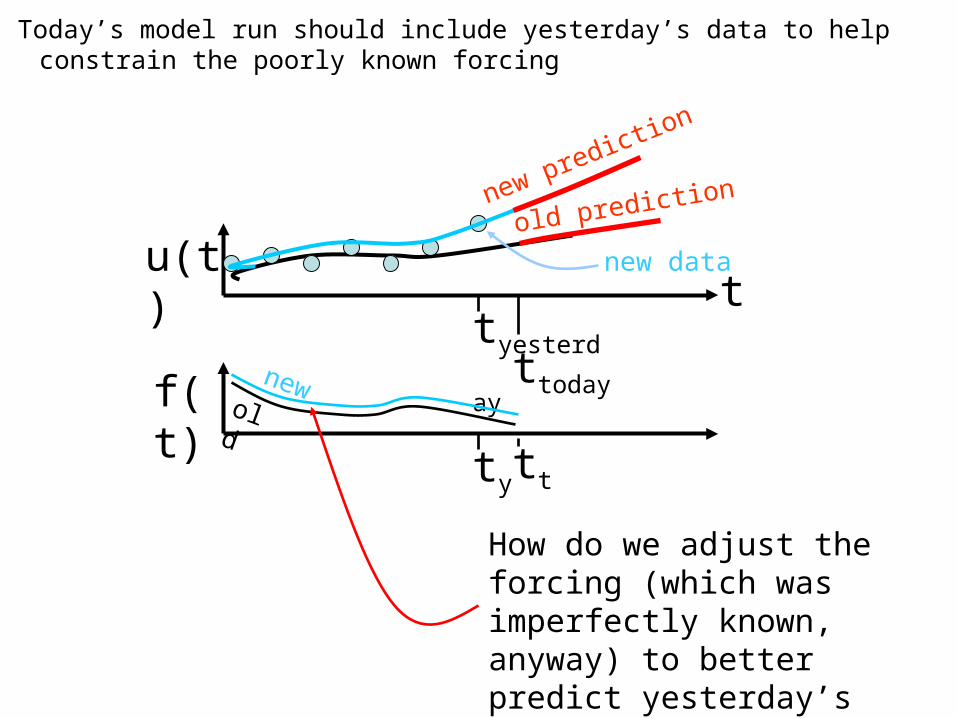
Today’s model run should include yesterday’s data to help constrain the poorly known forcing

tu(t)

tyesterday

f(t)

ty

old prediction

ttoday

tt

new data

How do we adjust the forcing (which was imperfectly known, anyway) to better predict yesterday’s weather?

new prediction

old

new

Part 2

The mathematics of

continuous functions

inner products

linear operators

and their

adjoints

Discrete

vectors uk and vk

Continuous

functions f(t) and g(t)

functions f(t) and g(t)

Discrete approximation as a vectors

uk=f(kt) and vk=g(kt)

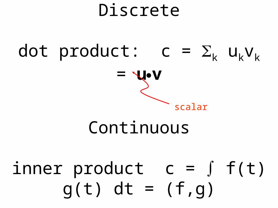
Discrete

dot product: c = k ukvk = uv

Continuous

inner product c = f(t) g(t) dt = (f,g)

scalar

discrete approximation as dot product

(f,g) = f(t) g(t) dt = t k ukvk = t uv

with uk=f(kt) and vk=g(kt)

inner product (f,g)

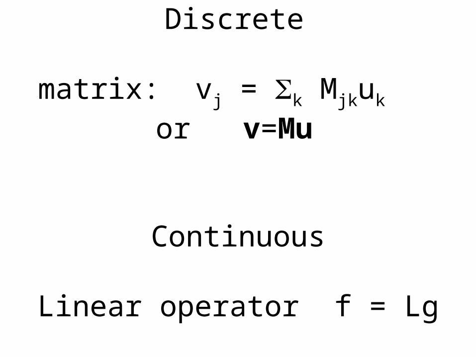
Discrete

matrix: vj = k Mjkuk or v=Mu

Continuous

Linear operator f = Lg

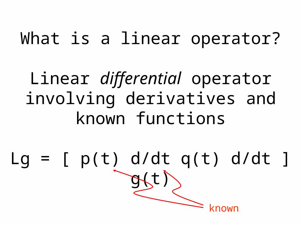
What is a linear operator?

Linear differential operatorinvolving derivatives and known functions

Lg = [ p(t) d/dt q(t) d/dt ] g(t)

known

and/or

Linear integral operatorinvolving intergral and known functions

Lg = p(t,t’) g(t’) dt’

known

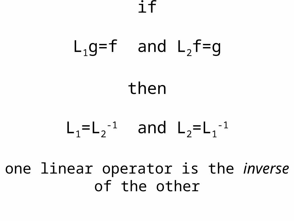
if

L1g=f and L2f=g

then

L1=L2-1 and L2=L1

-1

one linear operator is the inverse of the other

discrete approximations

1 0 0 0 … 0

-1 1 0 0 … 0

0 -1 1 0 … 0

……

… 0 0 -1 1

Lg=f with L = d/dtplus b.c. g(0)=known

Lg=f with Lg = 0

tg(t’)dt’

plus b.b. g(0)=known

Mu=v, M = t-1

1 0 0 0 … 0

1 1 0 0 … 0

1 1 1 0 … 0

……

… 1 1 1 1

Mu=v, M = t

Sample differential operator plus b.c.

Sample integral operator plus b.c.

Question concerning a dot product …

given two matrices A and B

when is (Au)v = u(Bv) ?

Answer: when B=AT, since

(Au)v = (Au)Tv = uTATv = uT(ATv) = u (ATv)

Question concerning an inner product …

given two linear operators L1 and L2

when is ( L1f , g ) = ( f, L2g ) ?

Answer: never mind, but let’s give it a name

(L1f, g) = (f, L2g) when L1 is the adjoint of L2

let’s denote the adjoint relationship L2=L1*

means “adjoint”

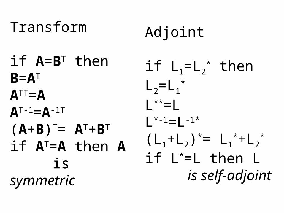
Transform

if A=BT then B=AT

ATT=AAT-1=A-1T

(A+B)T= AT+BT

if AT=A then A is symmetric

Adjoint

if L1=L2* then L2=L1

*

L**=LL*-1=L-1*

(L1+L2)*= L1*+L2

*

if L*=L then L is self-adjoint

Calculating adjoints by integration by parts

Let L = d/dtwith b.c. zero at ±

(Lf, g) = -+

df/dt g dt

= f g |-+

- -+

f dg/dt dt = - -+

f dg/dt dt

= (f, L*g)

So L* = -d/dtwith b.c. zero at ±

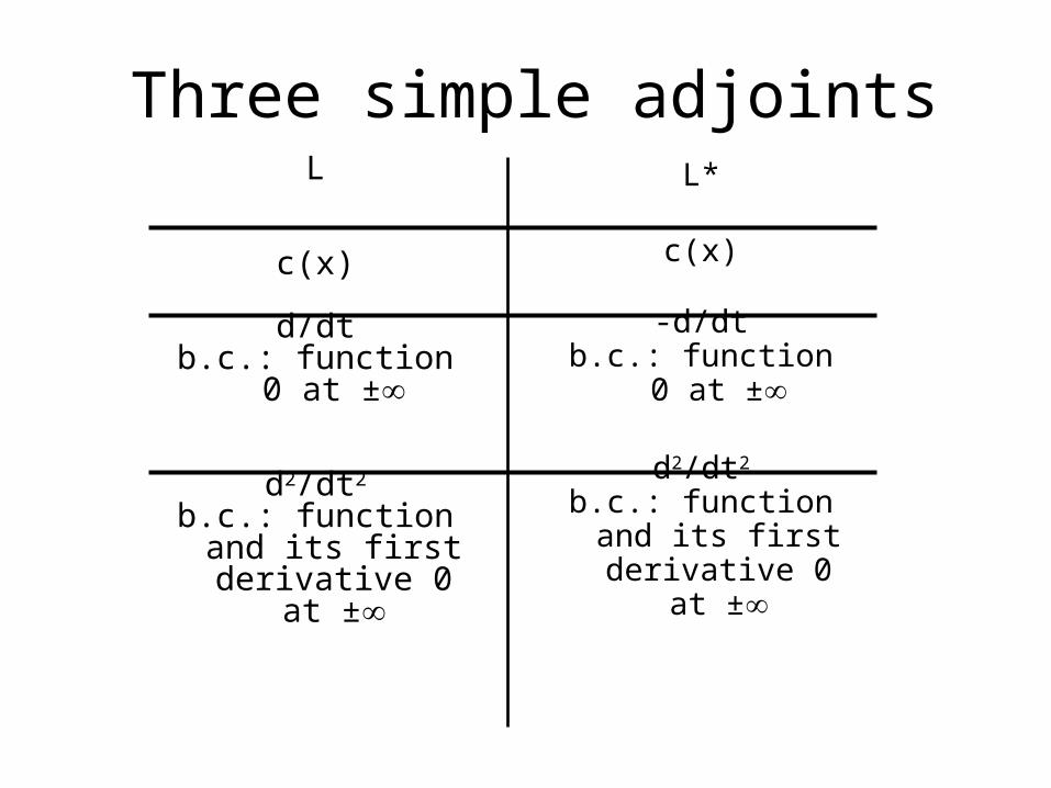
Three simple adjointsL

c(x)

d/dtb.c.: function 0 at

±

d2/dt2

b.c.: function and its first derivative 0

at ±

L*

c(x)

-d/dtb.c.: function 0 at

±

d2/dt2

b.c.: function and its first derivative 0

at ±

Part 3

Functional derivatives

How to represent

the idea that a perturbation in forcing, f(t)

cause a perturbation in response, u(t)

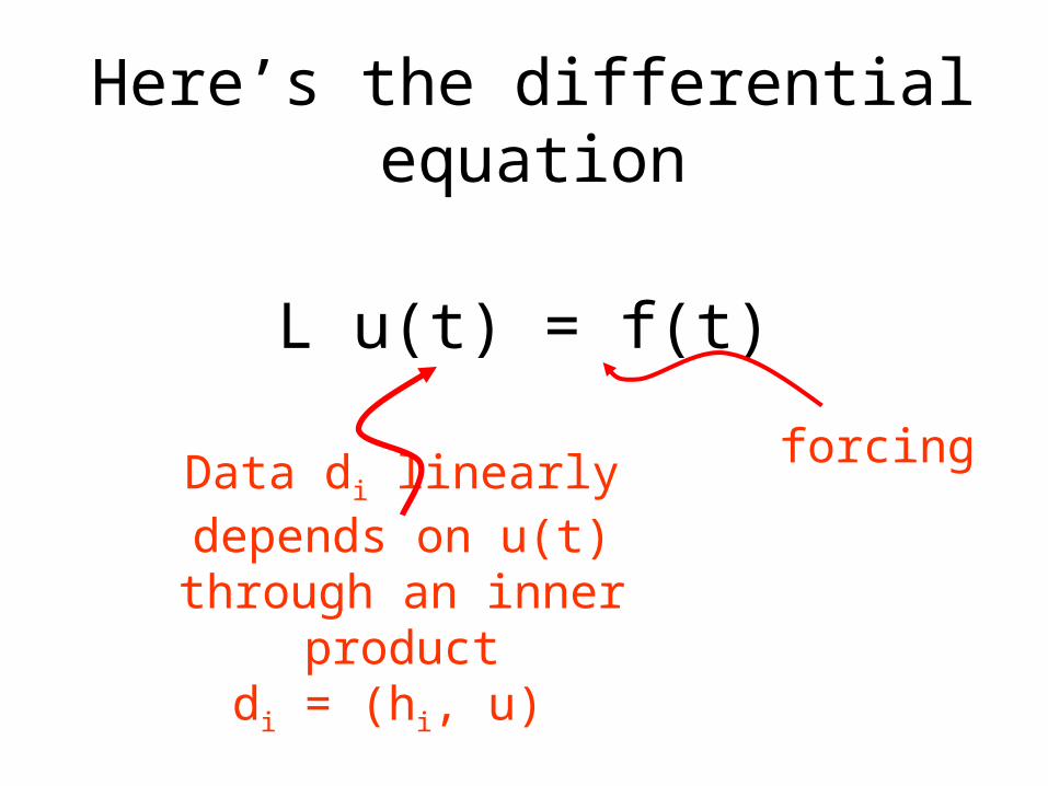
Here’s the differential equation

L u(t) = f(t)

forcing

Data di linearly depends on u(t)through an inner product

di = (hi, u)

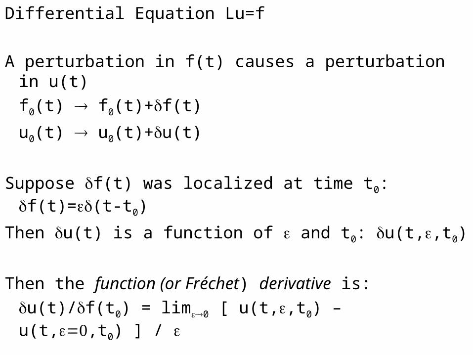
Differential Equation Lu=f

A perturbation in f(t) causes a perturbation in u(t)

f0(t) f0(t)+f(t)

u0(t) u0(t)+u(t)

Suppose f(t) was localized at time t0: f(t)=(t-t0)

Then u(t) is a function of and t0: u(t,,t0)

Then the function (or Fréchet) derivative is:

u(t)/f(t0) = lim0 [ u(t,,t0) – u(t,,t0) ] /

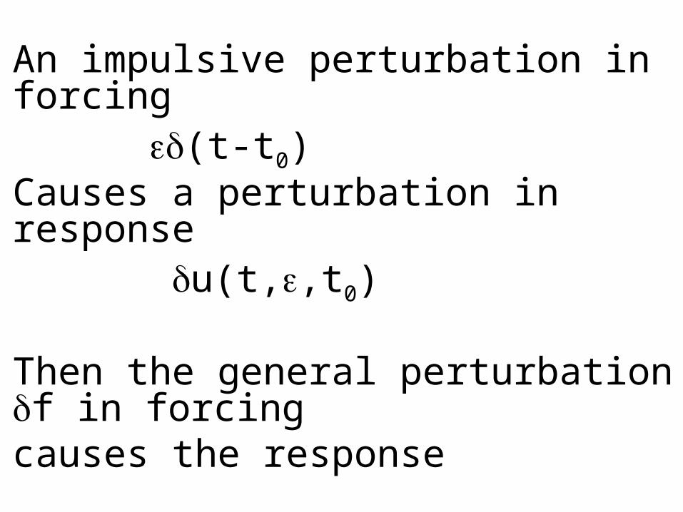
An impulsive perturbation in forcing(t-t0)

Causes a perturbation in response u(t,,t0)

Then the general perturbation f in forcingcauses the response

u = (u/f) f dt0 = ( u/f, f )

t(t-t0)

t0

u

t0

An impulsive perturbation in forcing

Causes this response

tf

t0

u

t0

A more complicated perturbation in forcing

Causes this response

definesu/a

u =u/a, a)

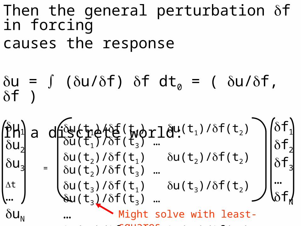
Then the general perturbation f in forcingcauses the response

u = (u/f) f dt0 = ( u/f, f )

In a discrete world:

u1

u2

u3 = t

…uN

u(t1)/f(t1) u(t1)/f(t2) u(t1)/f(t3) …u(t2)/f(t1) u(t2)/f(t2) u(t2)/f(t3) …u(t3)/f(t1) u(t3)/f(t2) u(t3)/f(t3) ……u(tN)/f(t1) u(tN)/f(t2) u(tN)/f(t3) …

f1

f2

f3

…fN

Might solve with least-squares …

Part 4

Calculating the data kernel

The functional derivative of

data

with respect to forcing

The Goal

to find the data kernel, gi(t)

which relates a perturbation in the data, di, to a perturbation in the forcing f(t)

through an inner product

di = ( gi(t), f(t) )

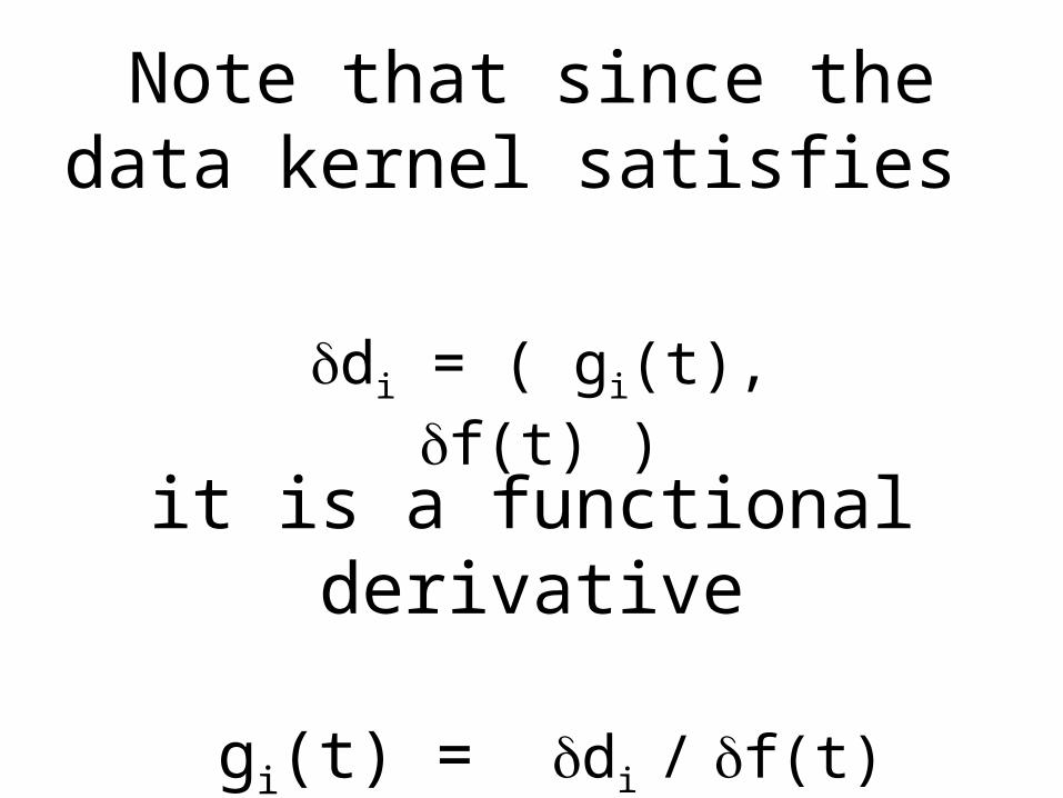
Note that since the data kernel satisfies

it is a functional derivative

gi(t) = di / f(t)

di = ( gi(t), f(t) )

Step 1:

assume that a function u(t) solves a linear differential equation with forcing f(t)

L u(t) = f(t)

Step 2:

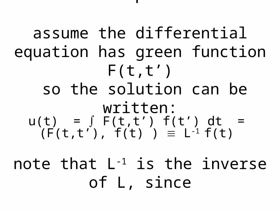
assume the differential equation has green function F(t,t’)

so the solution can be written:

note that L-1 is the inverse of L, since

f=Lu and u=L-1f

u(t) = F(t,t’) f(t’) dt = (F(t,t’), f(t) ) L-1 f(t)

Step 3:

assume that the data, di, are related to the solution u(t) through an inner product

di = ( hi(t), u(t) )

Step 4:

do some substitutions and manipulations

di = ( hi(t), u(t) )

= ( hi(t), L-1f(t) )

= (L-1*hi(t), f(t) )

= (L*-1hi(t), f(t) )

Step 4:since the problem is linear, this rule applies to perturbations of functions as well as to

the functions themselves

di = (L*-1hi(t), f(t) )

So

di = (L*-1hi(t), f(t) )

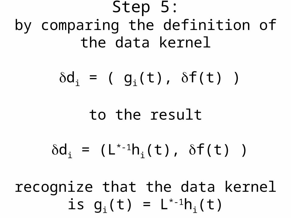
Step 5:by comparing the definition of the data kernel

di = ( gi(t), f(t) )

to the result

di = (L*-1hi(t), f(t) )

recognize that the data kernel is gi(t) = L*-1hi(t)

Step 6:

since the data kernel satisfies

gi(t) = L*-1hi(t)

then it must satisfy the differential equation

L*gi(t) = hi(t)

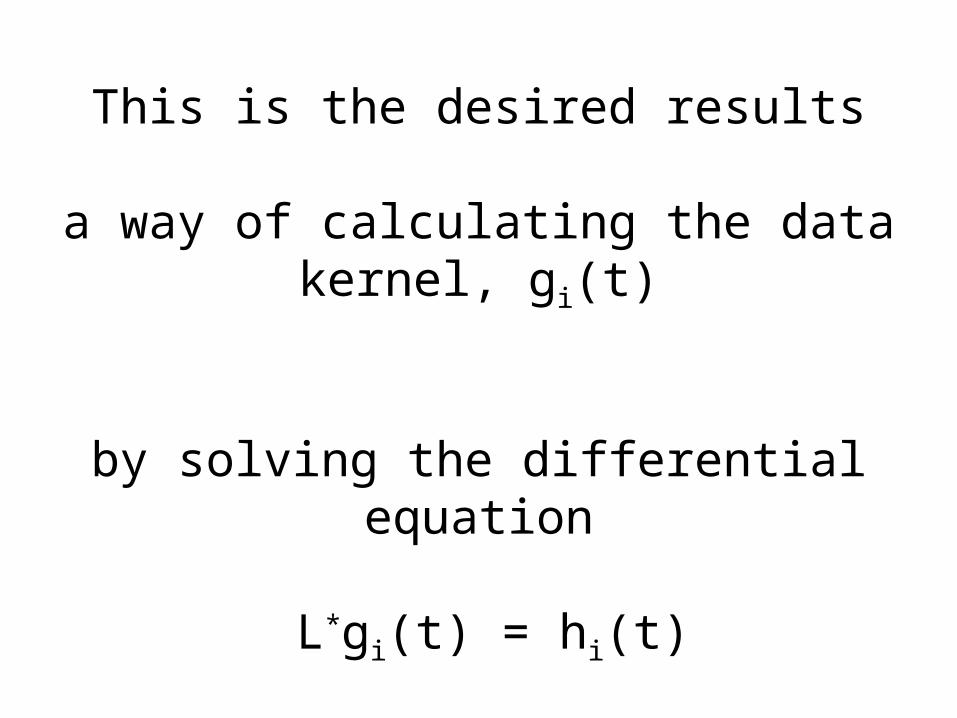
This is the desired results

a way of calculating the data kernel, gi(t)

by solving the differential equation

L*gi(t) = hi(t)

Part 5

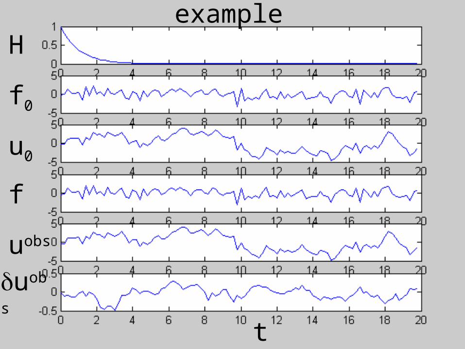
An example

Note: In this example I use very simple differential equations that can be solved analytically.

In a reality, you would be using much more complicated differential equations that but be solved numerically ..

Example: Newtonian cooling equation

du/dt + cu = f(t)

L = d/dt + c

u(t) is temperaturef(t) is heatingc is a constant

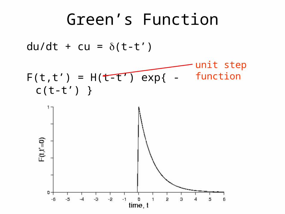
Green’s Function

du/dt + cu = (t-t’)

F(t,t’) = H(t-t’) exp{ -c(t-t’) }

unit step function

Adjoint differential equationL = d/dt + c

The adjoint of d/dt is –d/dtand the adjoint of c is c

So L* = -d/dt + c

And so du/dt + cu = f(t)

has corresponding adjoint equation

-dgi/dt + cgi = hi

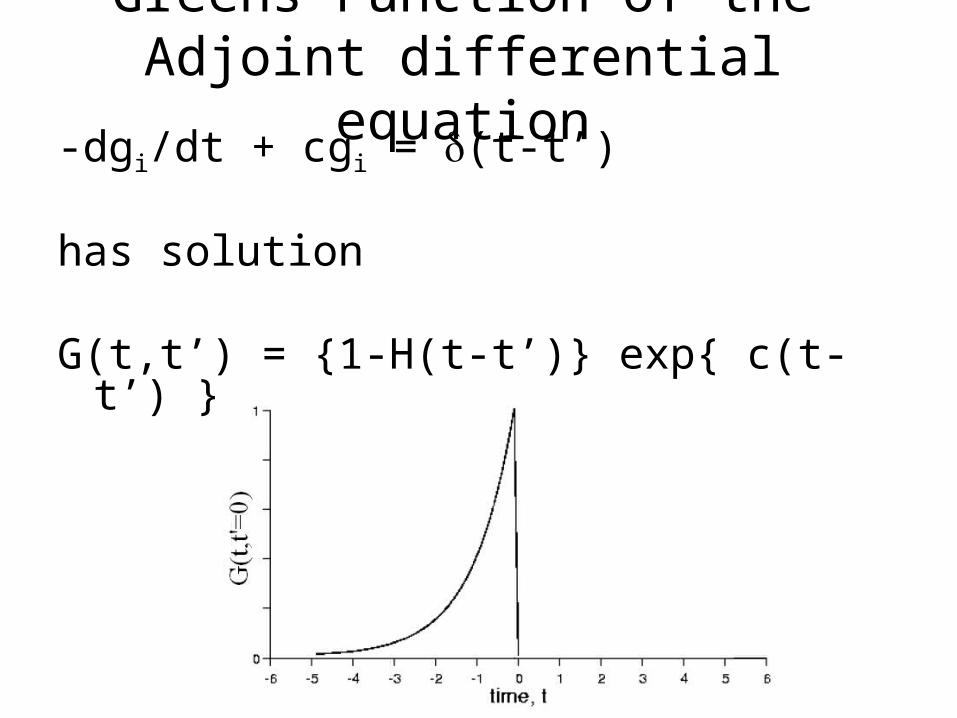
Greens Function of the Adjoint differential equation

-dgi/dt + cgi = (t-t’)

has solution

G(t,t’) = {1-H(t-t’)} exp{ c(t-t’) }

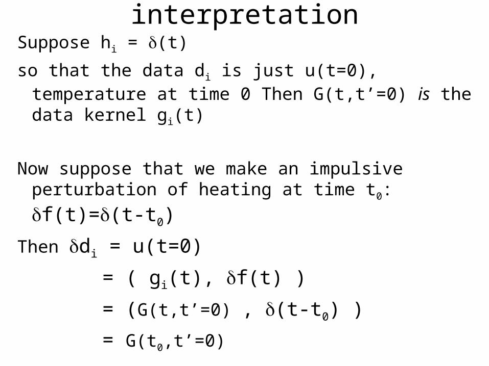
interpretationSuppose hi = (t)

so that the data di is just u(t=0), temperature at time 0 Then G(t,t’=0) is the data kernel gi(t)

Now suppose that we make an impulsive perturbation of heating at time t0: f(t)=(t-t0)

Then di = u(t=0)

= ( gi(t), f(t) )

= (G(t,t’=0) , (t-t0) )

= G(t0,t’=0)

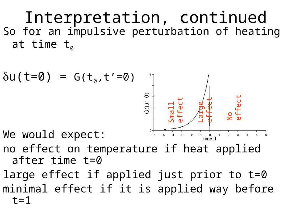
Interpretation, continuedSo for an impulsive perturbation of heating at time t0

u(t=0) = G(t0,t’=0)

We would expect:no effect on temperature if heat applied after time

t=0large effect if applied just prior to t=0minimal effect if it is applied way before t=1

No

effe

ct

Larg

e ef

fect

Sm

all e

ffec

t

exampleH

f0

u0

f

uobs

uobs

t

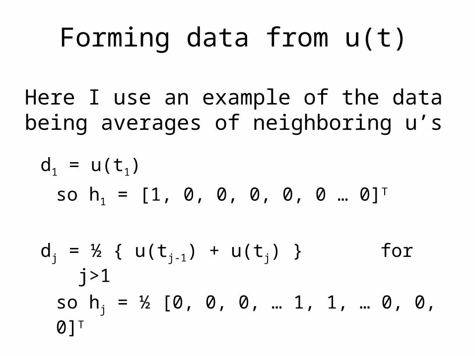
Forming data from u(t)

Here I use an example of the data being averages of neighboring u’s

d1 = u(t1)

so h1 = [1, 0, 0, 0, 0, 0 … 0]T

dj = ½ { u(tj-1) + u(tj) } for j>1

so hj = ½ [0, 0, 0, … 1, 1, … 0, 0, 0]T

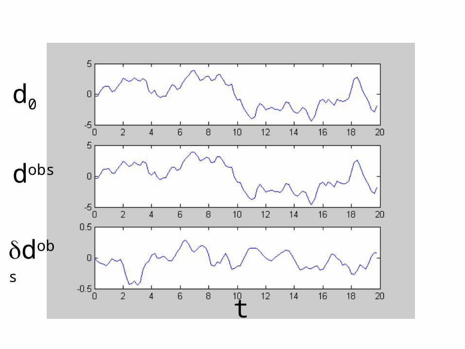
d0

dobs

t

dobs

The problem

Reconstruct f from d

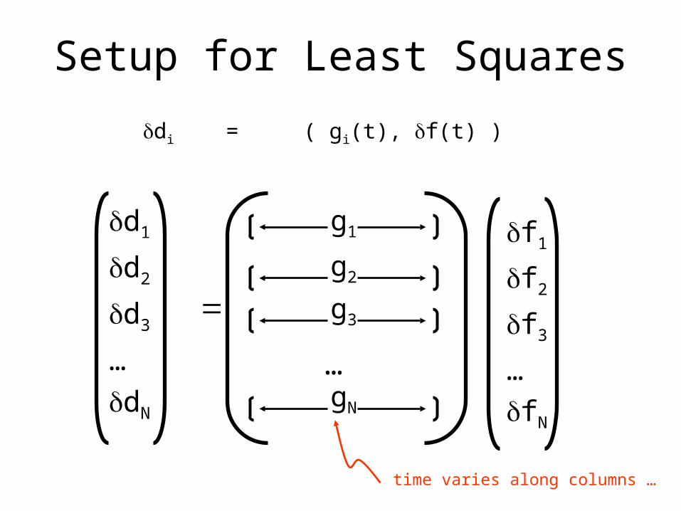
Setup for Least Squares

di = ( gi(t), f(t) )

f1

f2

f3

…

fN

d1

d2

d3

…

dN

g1

g2

g3

gN

…

time varies along columns …

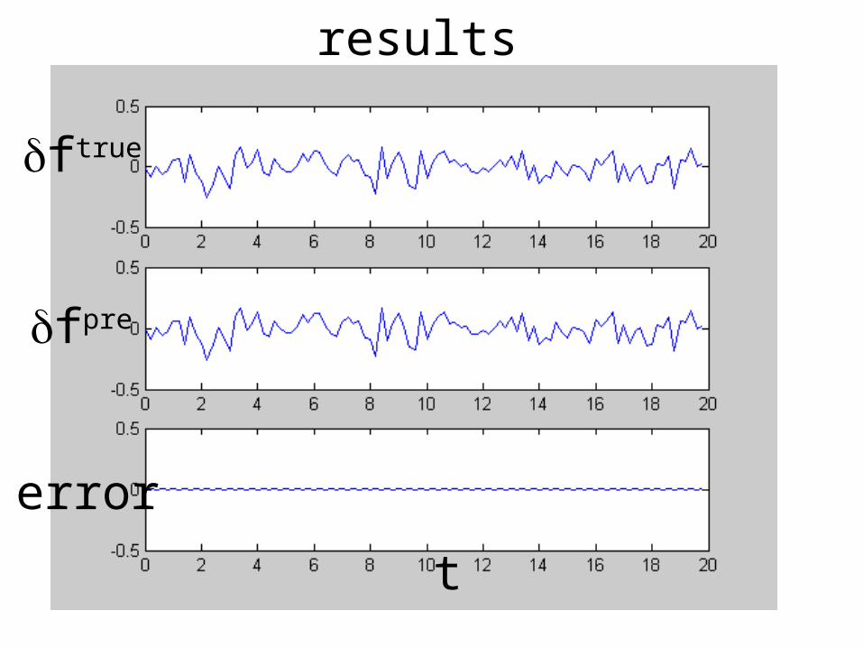
ftrue

error

t

fpre

results

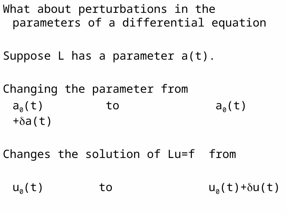
What about perturbations in the parameters of a differential equation

Suppose L has a parameter a(t).

Changing the parameter from

a0(t) to a0(t)+a(t)

Changes the solution of Lu=f from

u0(t) to u0(t)+u(t)

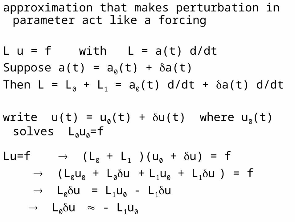
approximation that makes perturbation in parameter act like a forcing

L u = f with L = a(t) d/dt

Suppose a(t) = a0(t) + a(t)

Then L = L0 + L1 = a0(t) d/dt + a(t) d/dt

write u(t) = u0(t) + u(t) where u0(t) solves L0u0=f

Lu=f (L0 + L1 )(u0 + u) = f

(L0u0 + L0u + L1u0 + L1u ) = f

L0u = L1u0 - L1u

L0u - L1u0

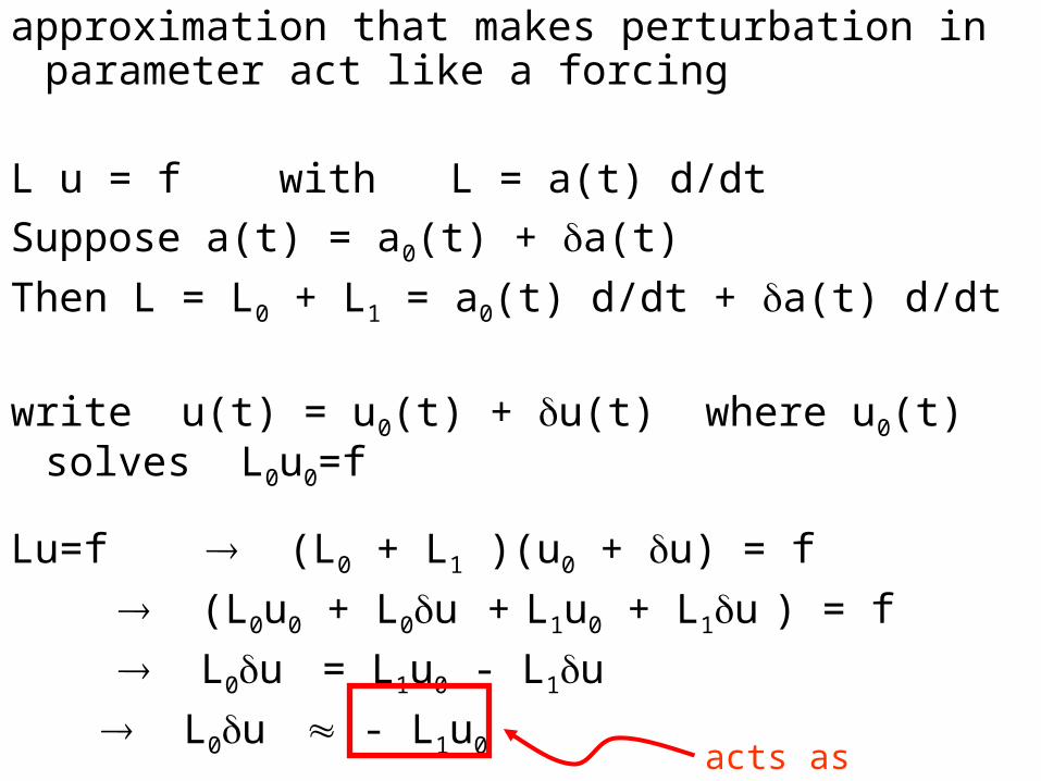
approximation that makes perturbation in parameter act like a forcing

L u = f with L = a(t) d/dt

Suppose a(t) = a0(t) + a(t)

Then L = L0 + L1 = a0(t) d/dt + a(t) d/dt

write u(t) = u0(t) + u(t) where u0(t) solves L0u0=f

Lu=f (L0 + L1 )(u0 + u) = f

(L0u0 + L0u + L1u0 + L1u ) = f

L0u = L1u0 - L1u

L0u - L1u0 acts as forcing