Embed Size (px)
Citation preview
Lecture 2.1 - Image Processing Image filtering
Idar Dyrdal
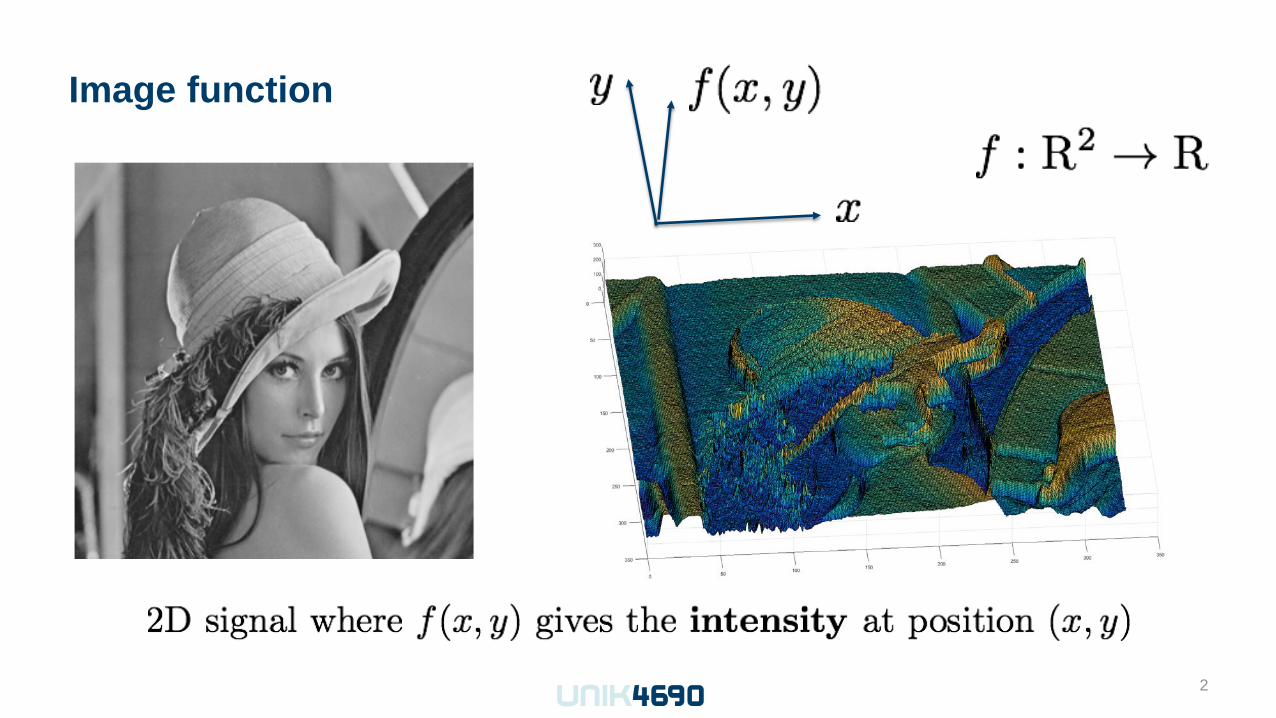
Image function
2
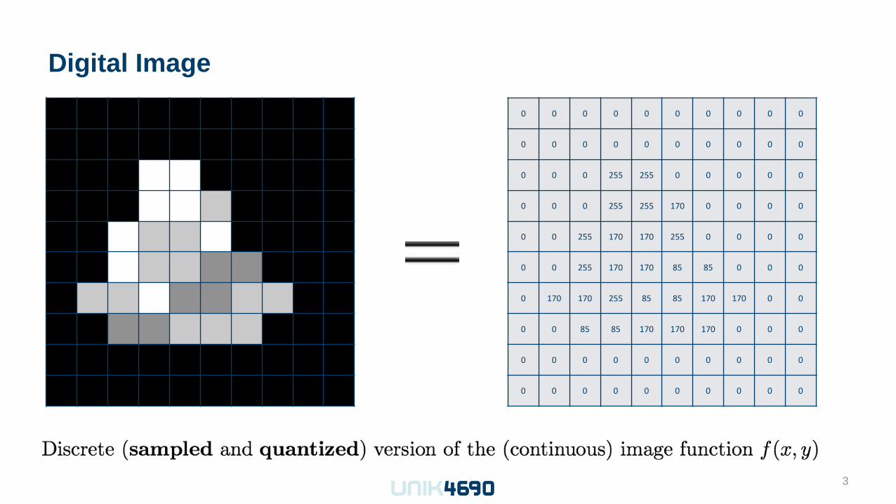
Digital Image
3
0 0 0 0 0 0 0 0 0 0
0 0 0 0 0 0 0 0 0 0
0 0 0 255 255 0 0 0 0 0
0 0 0 255 255 170 0 0 0 0
0 0 255 170 170 255 0 0 0 0
0 0 255 170 170 85 85 0 0 0
0 170 170 255 85 85 170 170 0 0
0 0 85 85 170 170 170 0 0 0
0 0 0 0 0 0 0 0 0 0
0 0 0 0 0 0 0 0 0 0

Image Processing
• Point operators
• Image filtering in spatial domain - Linear filters - Non-linear filters
• Image filtering in frequency domain - Fourier transform
4
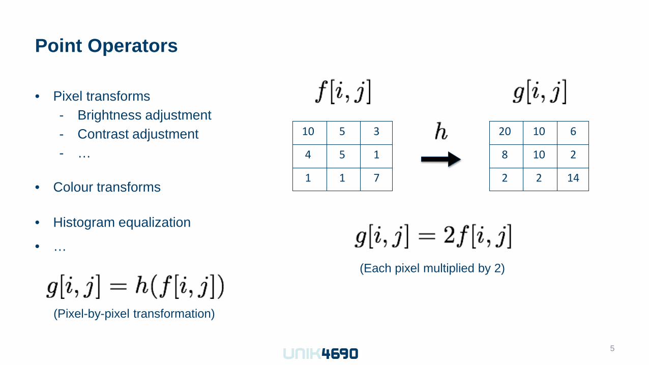
Point Operators
• Pixel transforms - Brightness adjustment - Contrast adjustment - …
• Colour transforms
• Histogram equalization
• …
5
(Each pixel multiplied by 2)
5 1 4
1 7 1
5 3 10
10 2 8
2 14 2
10 6 20
(Pixel-by-pixel transformation)
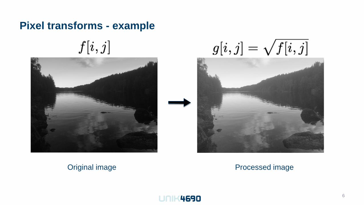
Pixel transforms - example
Original image Processed image
6
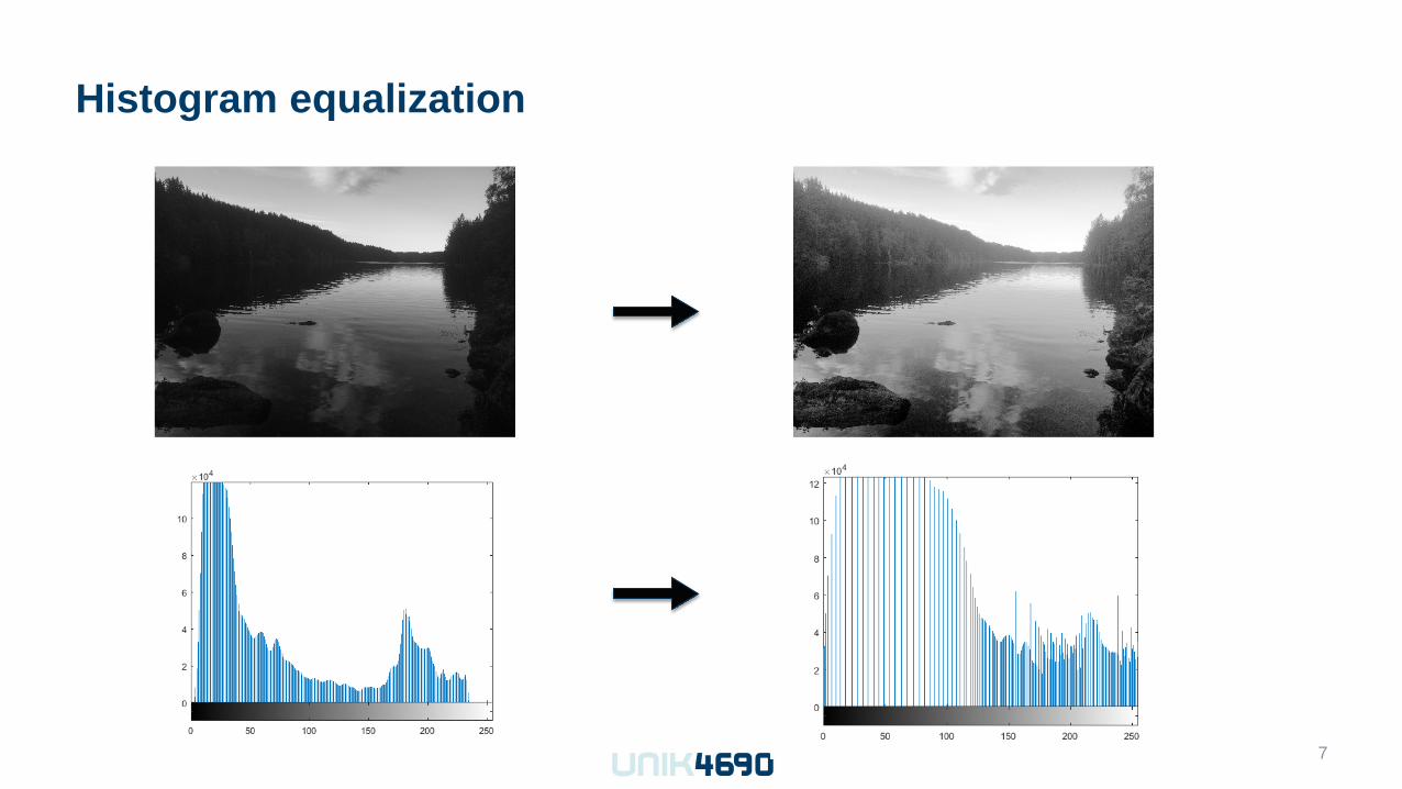
Histogram equalization
7
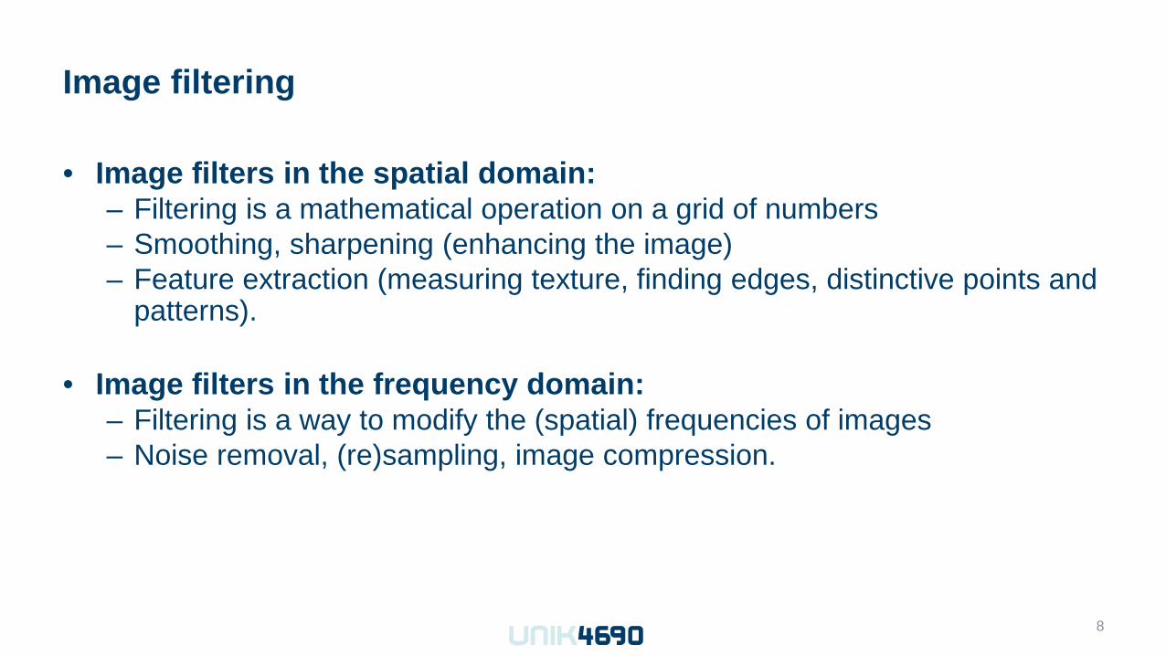
Image filtering
• Image filters in the spatial domain: – Filtering is a mathematical operation on a grid of numbers – Smoothing, sharpening (enhancing the image) – Feature extraction (measuring texture, finding edges, distinctive points and
patterns).
• Image filters in the frequency domain: – Filtering is a way to modify the (spatial) frequencies of images – Noise removal, (re)sampling, image compression.
8
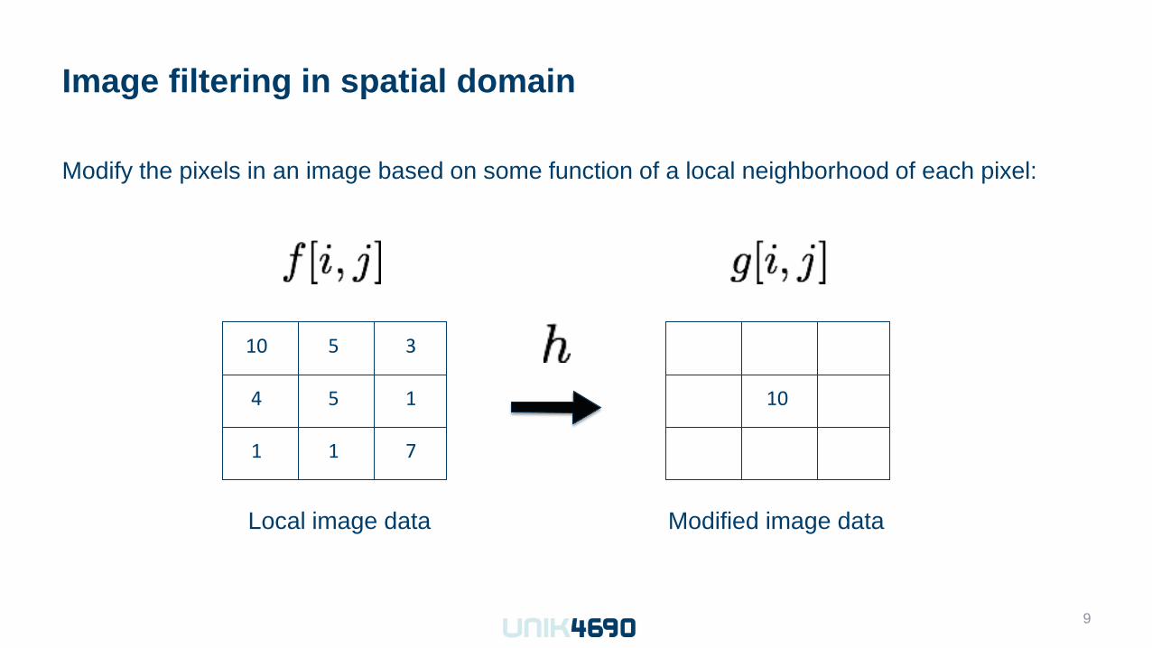
Image filtering in spatial domain
Modify the pixels in an image based on some function of a local neighborhood of each pixel:
9
5 1 4
1 7 1
5 3 10
10
Local image data Modified image data
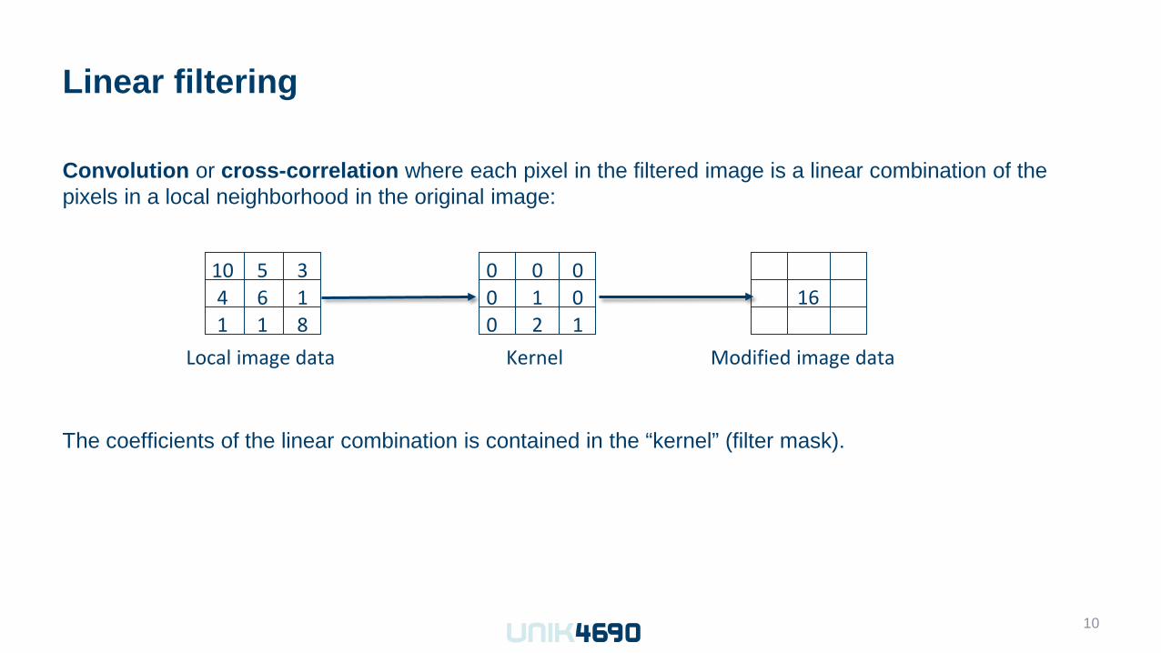
Linear filtering
Convolution or cross-correlation where each pixel in the filtered image is a linear combination of the pixels in a local neighborhood in the original image:
10
1 1 0 0 2 0
0 0 0
Kernel Modified image data Local image data
16 6 1 4 1 8 1
5 3 10
The coefficients of the linear combination is contained in the “kernel” (filter mask).
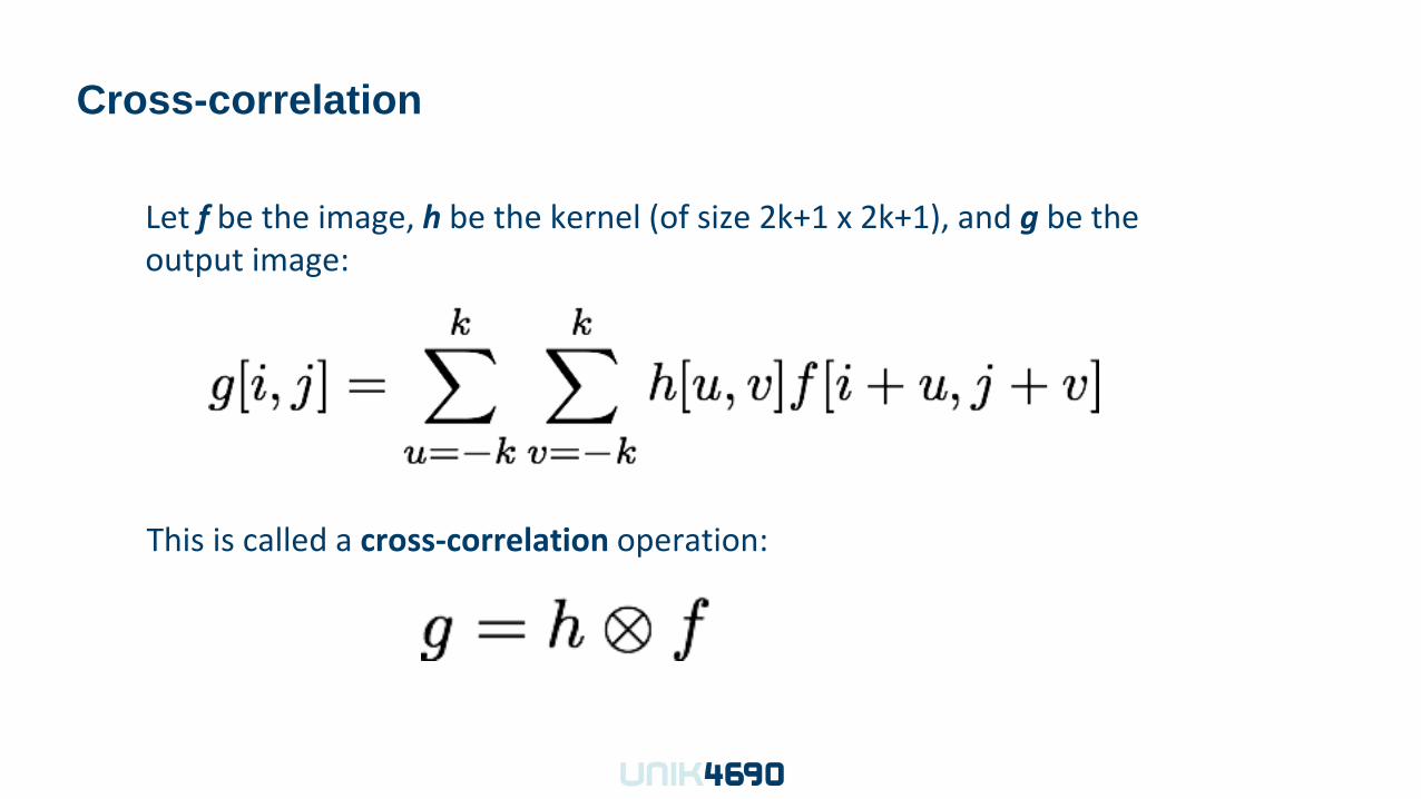
Cross-correlation
This is called a cross-correlation operation:
Let f be the image, h be the kernel (of size 2k+1 x 2k+1), and g be the output image:
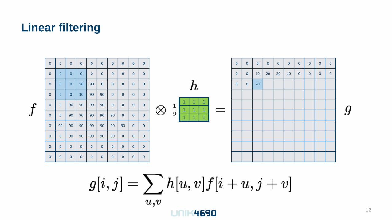
Linear filtering
12
0 0 0 0 0 0 0 0 0 0
0 0 0 0 0 0 0 0 0 0
0 0 0 90 90 0 0 0 0 0
0 0 0 90 90 90 0 0 0 0
0 0 90 90 90 90 0 0 0 0
0 0 90 90 90 90 90 0 0 0
0 90 90 90 90 90 90 90 0 0
0 0 90 90 90 90 90 0 0 0
0 0 0 0 0 0 0 0 0 0
0 0 0 0 0 0 0 0 0 0
0 0 0 0 0 0 0 0 0 0
0 0 10 20 20 10 0 0 0 0
0 0 20
1 1 1 1 1 1 1 1 1
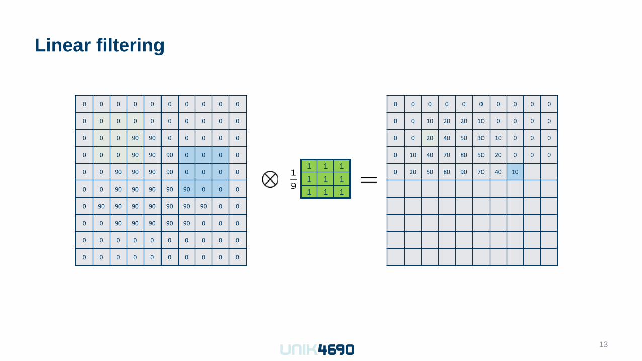
Linear filtering
13
0 0 0 0 0 0 0 0 0 0
0 0 0 0 0 0 0 0 0 0
0 0 0 90 90 0 0 0 0 0
0 0 0 90 90 90 0 0 0 0
0 0 90 90 90 90 0 0 0 0
0 0 90 90 90 90 90 0 0 0
0 90 90 90 90 90 90 90 0 0
0 0 90 90 90 90 90 0 0 0
0 0 0 0 0 0 0 0 0 0
0 0 0 0 0 0 0 0 0 0
0 0 0 0 0 0 0 0 0 0
0 0 10 20 20 10 0 0 0 0
0 0 20 40 50 30 10 0 0 0
0 10 40 70 80 50 20 0 0 0
0 20 50 80 90 70 40 10
1 1 1 1 1 1 1 1 1

Linear filtering
14
0 0 0 0 0 0 0 0 0 0
0 0 0 0 0 0 0 0 0 0
0 0 0 90 90 0 0 0 0 0
0 0 0 90 90 90 0 0 0 0
0 0 90 90 90 90 0 0 0 0
0 0 90 90 90 90 90 0 0 0
0 90 90 90 90 90 90 90 0 0
0 0 90 90 90 90 90 0 0 0
0 0 0 0 0 0 0 0 0 0
0 0 0 0 0 0 0 0 0 0
0 0 0 0 0 0 0 0 0 0
0 0 10 20 20 10 0 0 0 0
0 0 20 40 50 30 10 0 0 0
0 10 40 70 80 50 20 0 0 0
0 20 50 80 90 70 40 10 0 0
0 40 70 90 90 80 60 30 10 0
10 40 70 90 90 90 70 40 10 0
0 30 50 60 60 60 50 30 10 0
0 10 20 30 30 30 20 10 0 0
0 0 0 0 0 0 0 0 0 0
1 1 1 1 1 1 1 1 1
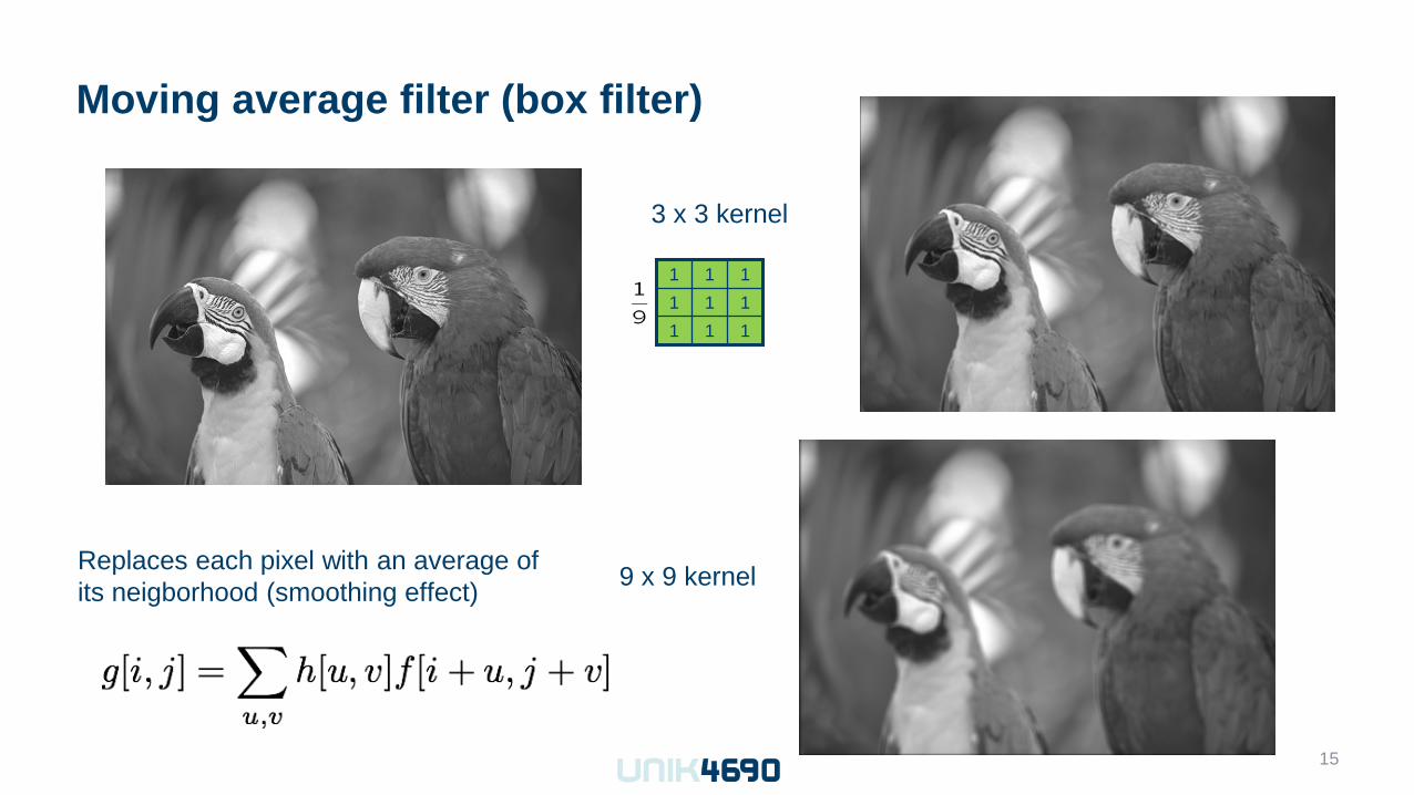
Moving average filter (box filter)
15
1 1 1 1 1 1 1 1 1
9 x 9 kernel
3 x 3 kernel
Replaces each pixel with an average of its neigborhood (smoothing effect)
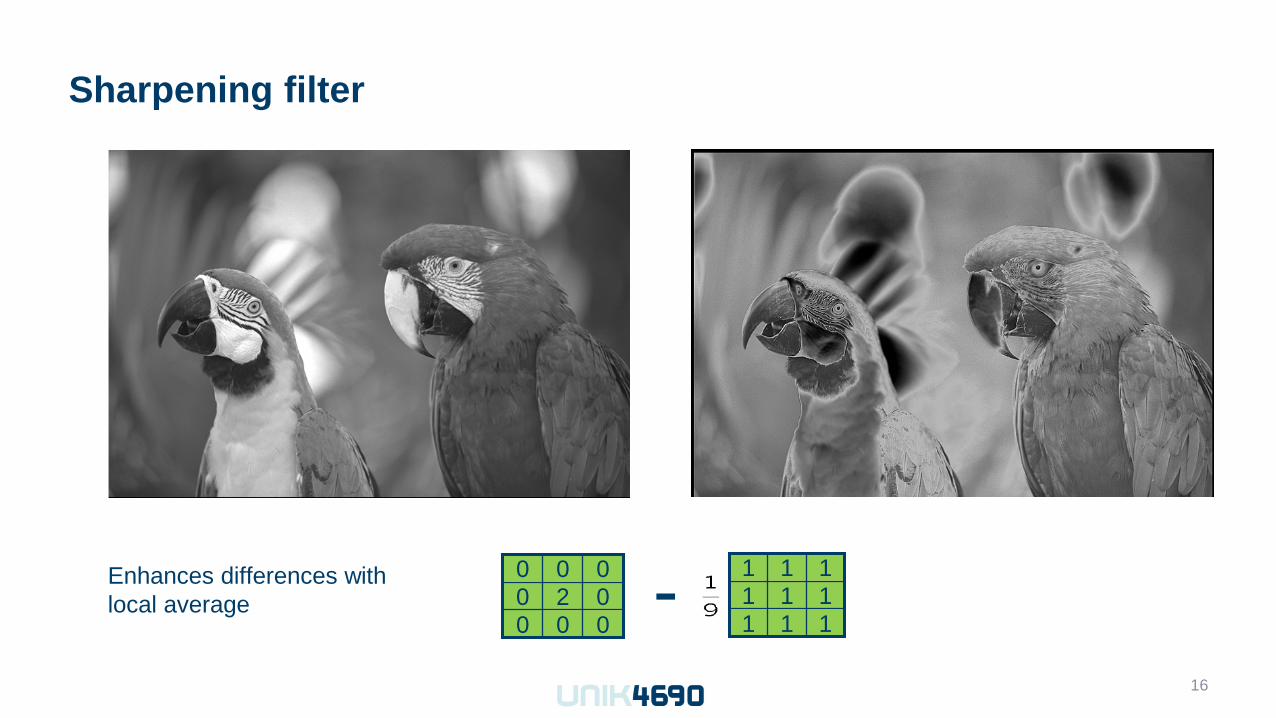
Sharpening filter
16
1 1 1 1 1 1 1 1 1
0 0 0 0 2 0 0 0 0 - Enhances differences with
local average
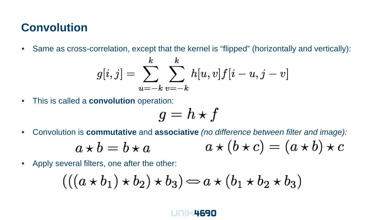
Convolution
• Same as cross-correlation, except that the kernel is “flipped” (horizontally and vertically):
• This is called a convolution operation:
• Convolution is commutative and associative (no difference between filter and image):
• Apply several filters, one after the other:
< >
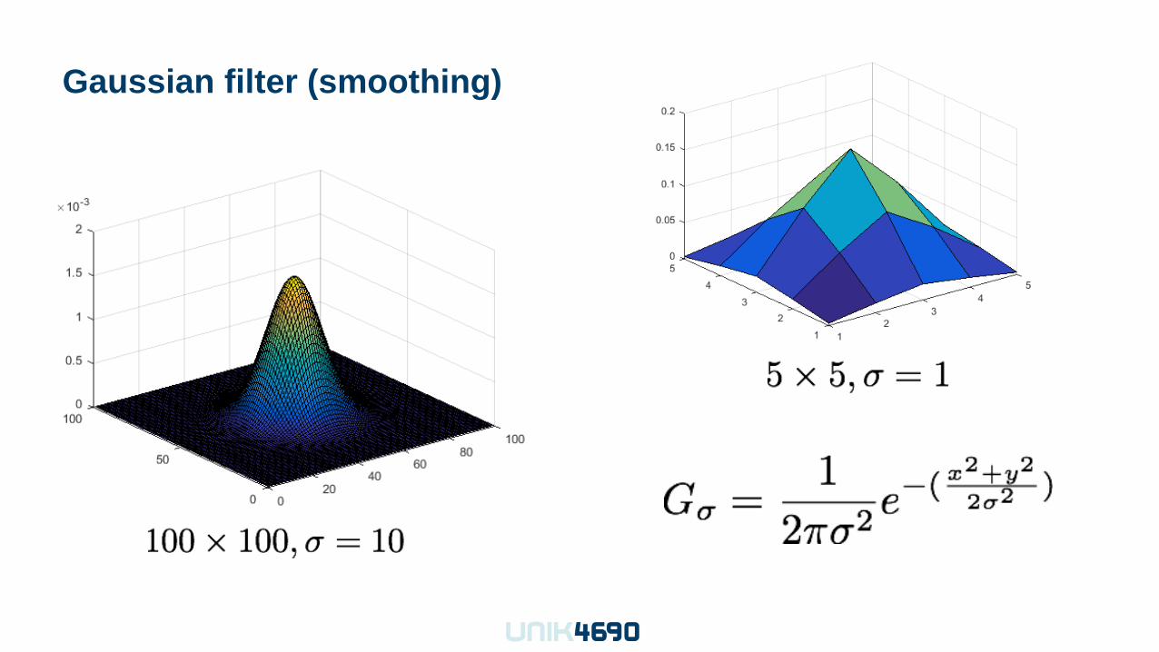
Gaussian filter (smoothing)
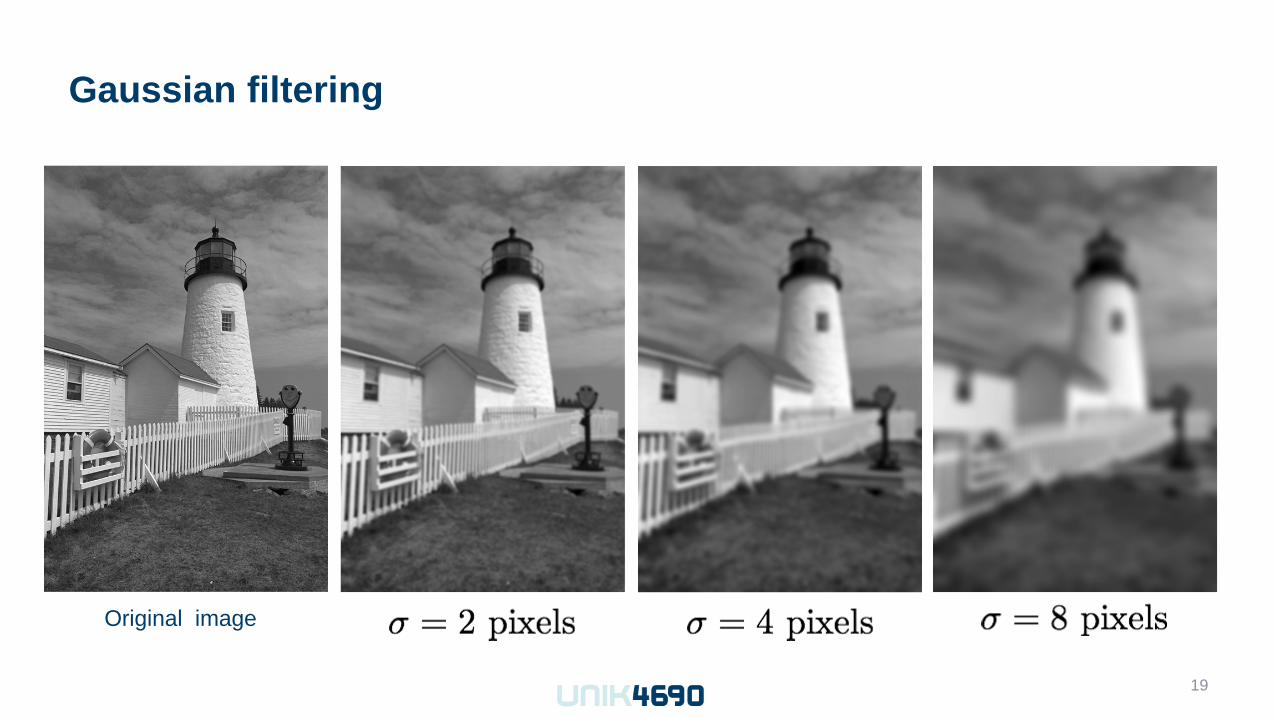
Gaussian filtering
Original image
19

Edge detection
20
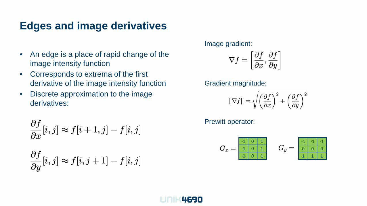
Edges and image derivatives
• An edge is a place of rapid change of the image intensity function
• Corresponds to extrema of the first derivative of the image intensity function
• Discrete approximation to the image derivatives:
Image gradient:
Gradient magnitude:
Prewitt operator:
1 0 -1 1 0 -1 1 0 -1
1 1 1 0 0 0 -1 -1 -1
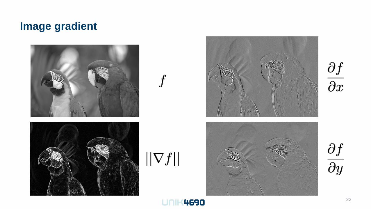
Image gradient
22
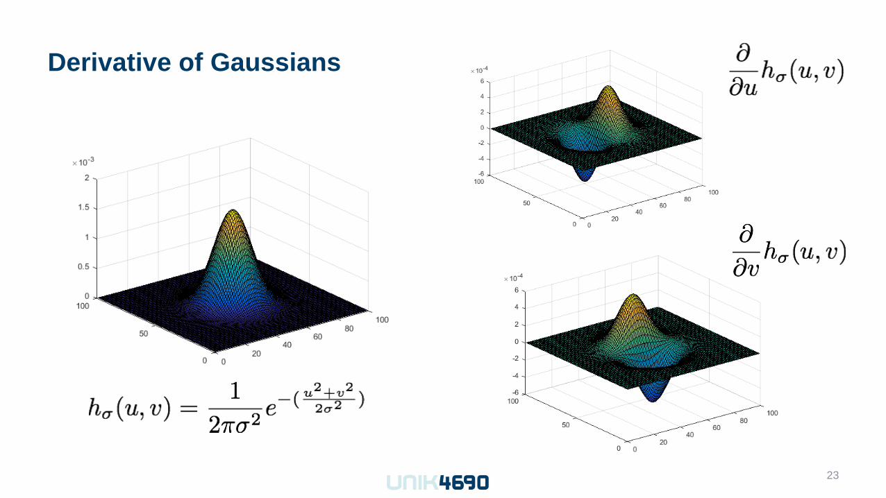
Derivative of Gaussians
23
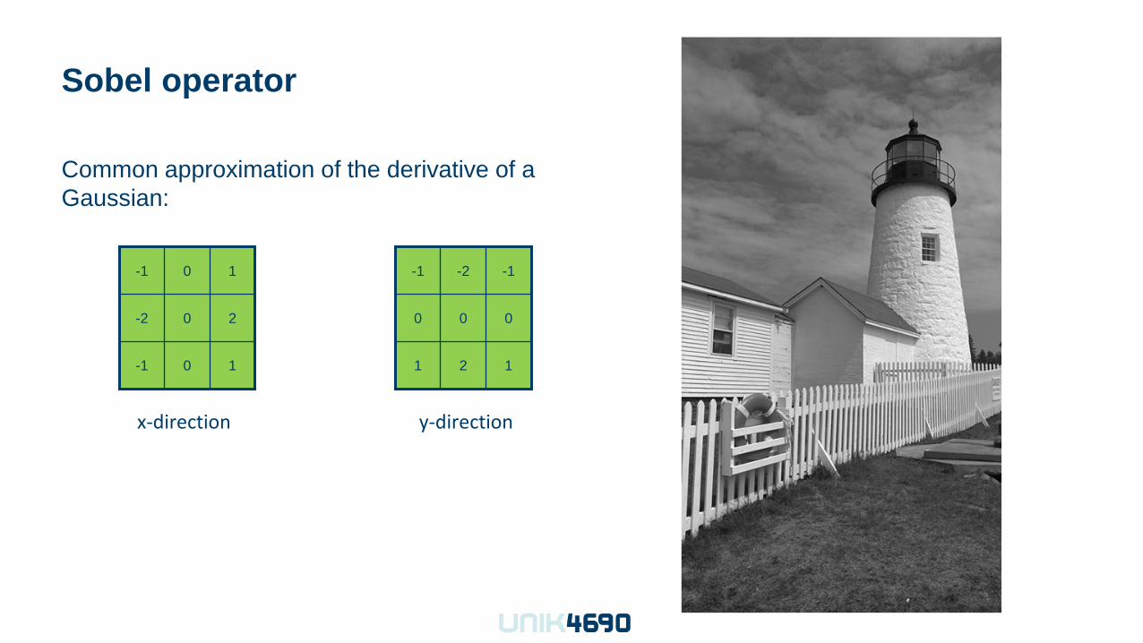
Sobel operator
Common approximation of the derivative of a Gaussian:
1 0 -1
2 0 -2
1 0 -1
1 2 1
0 0 0
-1 -2 -1
x-direction y-direction
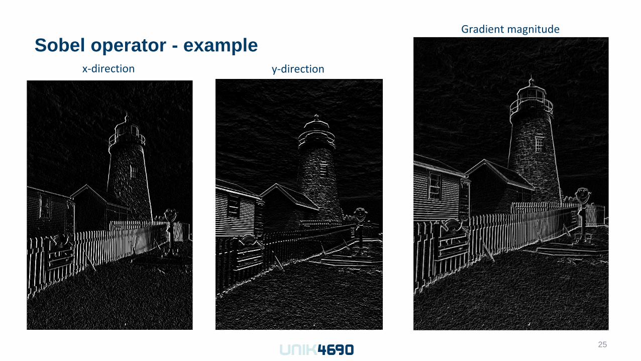
Sobel operator - example
25
x-direction y-direction
Gradient magnitude
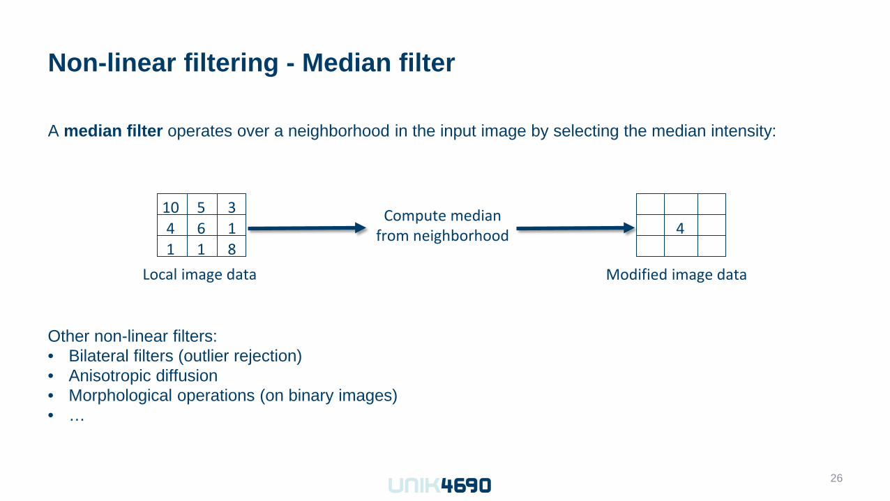
Non-linear filtering - Median filter
A median filter operates over a neighborhood in the input image by selecting the median intensity:
26
Compute median from neighborhood
Modified image data Local image data
4 6 1 4 1 8 1
5 3 10
Other non-linear filters: • Bilateral filters (outlier rejection) • Anisotropic diffusion • Morphological operations (on binary images) • …
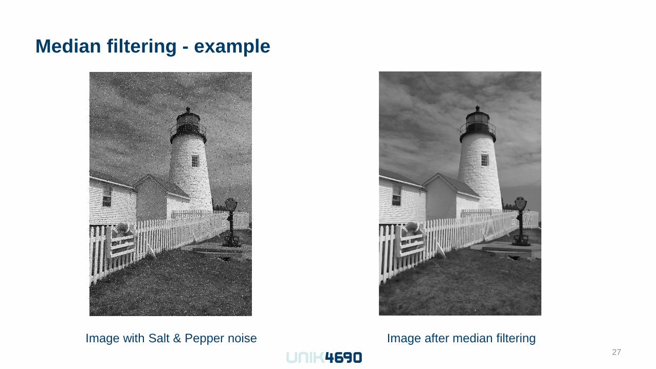
Median filtering - example
27 Image with Salt & Pepper noise Image after median filtering
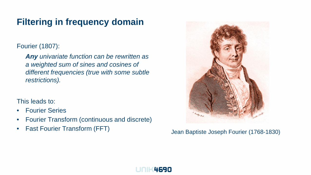
Filtering in frequency domain
Fourier (1807): Any univariate function can be rewritten as
a weighted sum of sines and cosines of different frequencies (true with some subtle restrictions).
This leads to: • Fourier Series • Fourier Transform (continuous and discrete) • Fast Fourier Transform (FFT) Jean Baptiste Joseph Fourier (1768-1830)

Sum of sines
+ + =
The Fourier transform stores the magnitude and phase at each frequency Amplitude: Phase:
Frequency
Amplitude
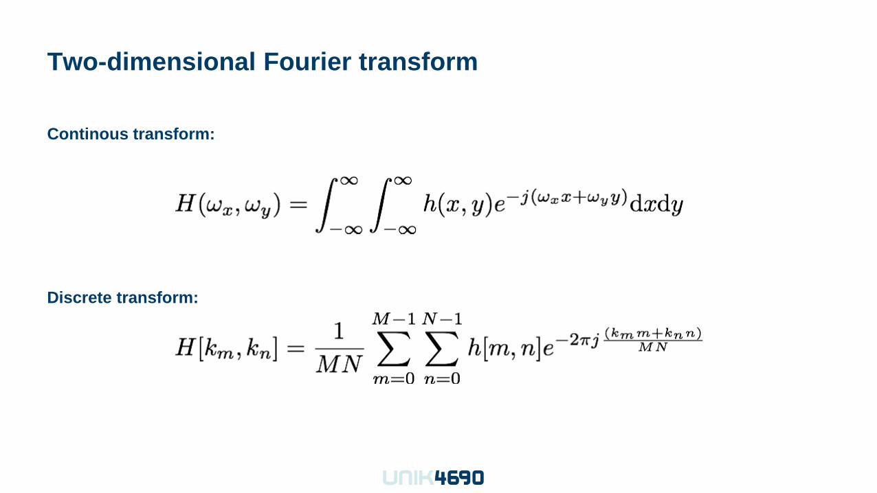
Two-dimensional Fourier transform
Continous transform: Discrete transform:
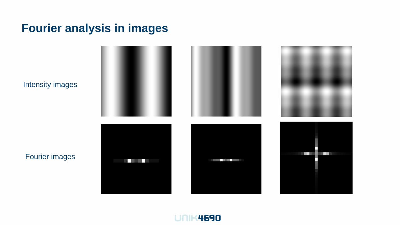
Fourier analysis in images
Intensity images
Fourier images
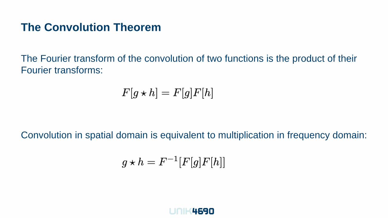
The Convolution Theorem
The Fourier transform of the convolution of two functions is the product of their Fourier transforms:
Convolution in spatial domain is equivalent to multiplication in frequency domain:
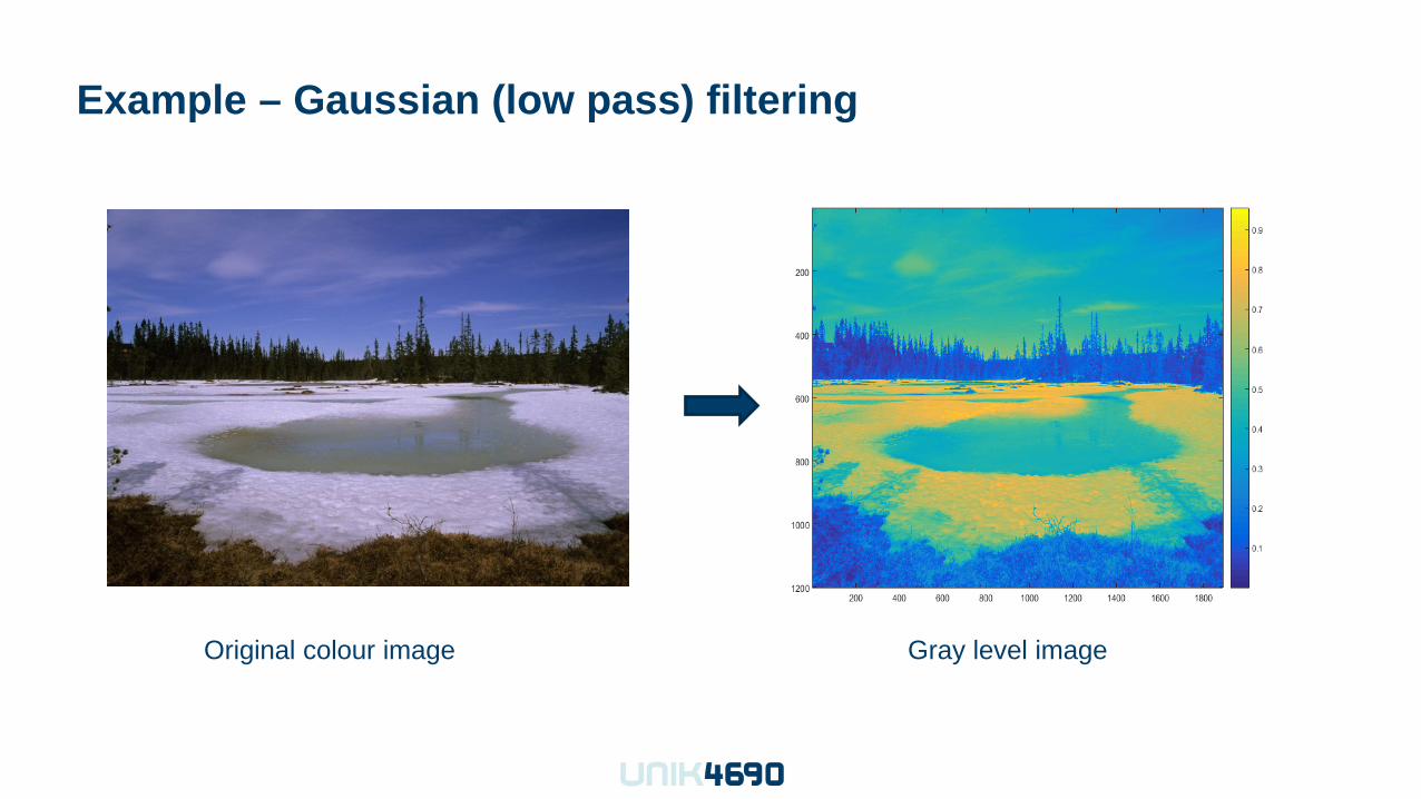
Example – Gaussian (low pass) filtering
Original colour image Gray level image
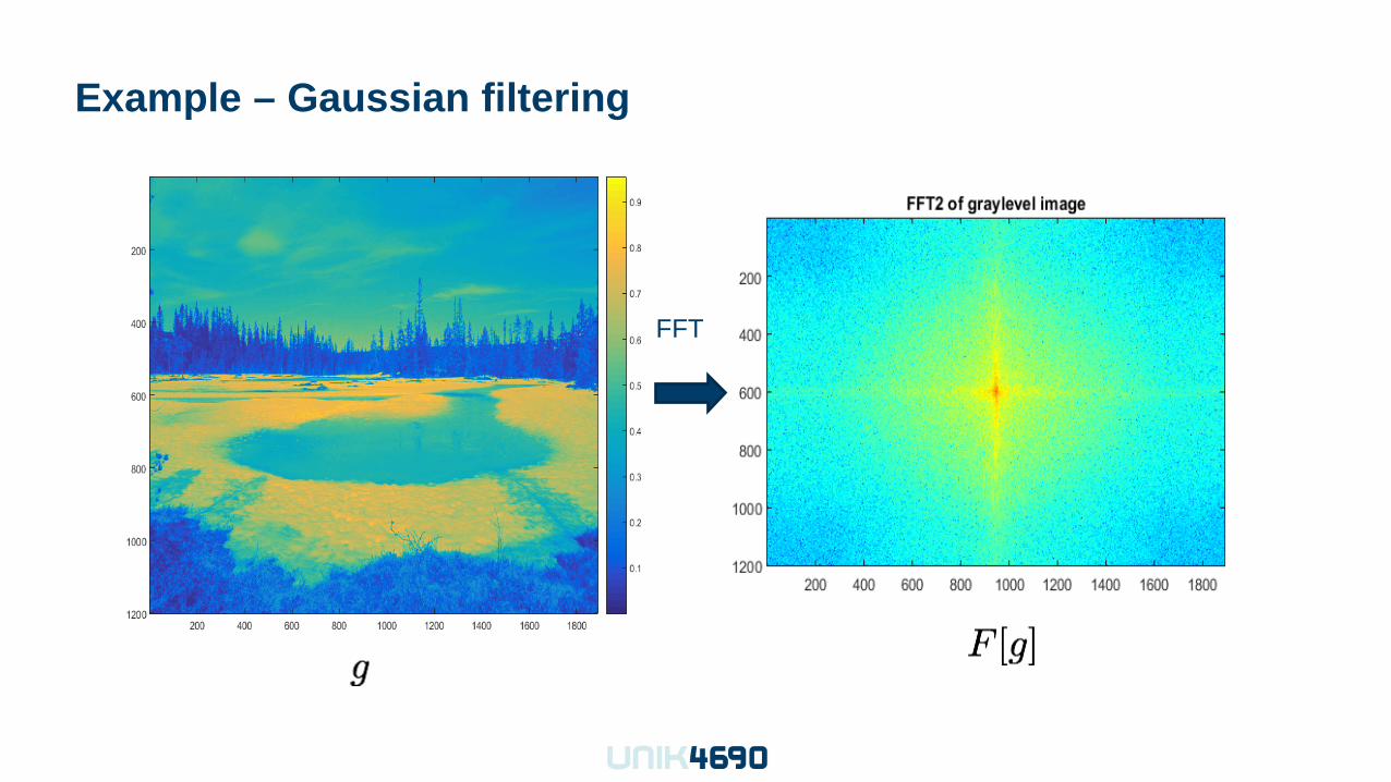
Example – Gaussian filtering
FFT
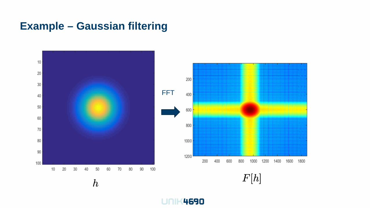
Example – Gaussian filtering
FFT
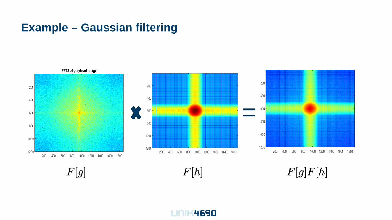
Example – Gaussian filtering
=
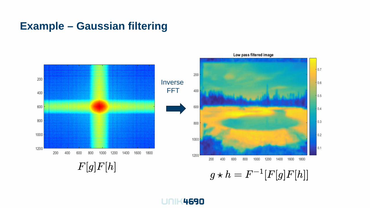
Example – Gaussian filtering
Inverse FFT
Summary
• Point operators • Image filtering in spatial domain
– Linear filters – Non-linear filters
• Image filtering in frequency domain
– Fourier transforms – Gaussian (low pass) filtering
• Szeliski 3.1 – 3.4