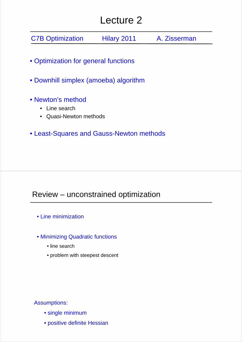
Lecture 2

C7B Optimization Hilary 2011 A. Zisserman

• Optimization for general functions

• Downhill simplex (amoeba) algorithm

• Newton’s method• Line search

• Quasi-Newton methods

• Least-Squares and Gauss-Newton methods

Review – unconstrained optimization

• Line minimization

• Minimizing Quadratic functions

• line search

• problem with steepest descent

Assumptions:

• single minimum

• positive definite Hessian

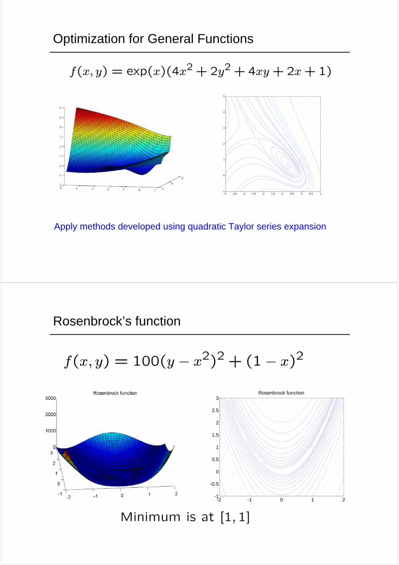
Optimization for General Functions

-4 -3.5 -3 -2.5 -2 -1.5 -1 -0.5 0 0.5 1-1

0

1

2

3

4

5

f(x, y) = exp(x)(4x2 + 2y2 + 4xy+2x+1)

Apply methods developed using quadratic Taylor series expansion

Rosenbrock’s function

f(x, y) = 100(y − x2)2 + (1− x)2

-2 -1 0 1 2-1

-0.5

0

0.5

1

1.5

2

2.5

3Rosenbrock function

Minimum is at [1,1]

-0.95 -0.9 -0.85 -0.8 -0.75

0.65

0.7

0.75

0.8

0.85

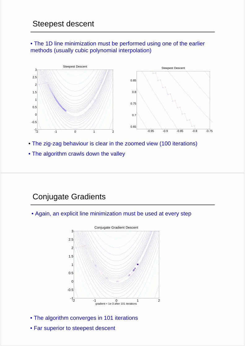
Steepest Descent

-2 -1 0 1 2-1

-0.5

0

0.5

1

1.5

2

2.5

3Steepest Descent

Steepest descent

• The zig-zag behaviour is clear in the zoomed view (100 iterations)

• The algorithm crawls down the valley

• The 1D line minimization must be performed using one of the earlier methods (usually cubic polynomial interpolation)

Conjugate Gradients

• Again, an explicit line minimization must be used at every step

• The algorithm converges in 101 iterations

• Far superior to steepest descent

-2 -1 0 1 2-1

-0.5

0

0.5

1

1.5

2

2.5

3Conjugate Gradient Descent

gradient < 1e-3 after 101 iterations

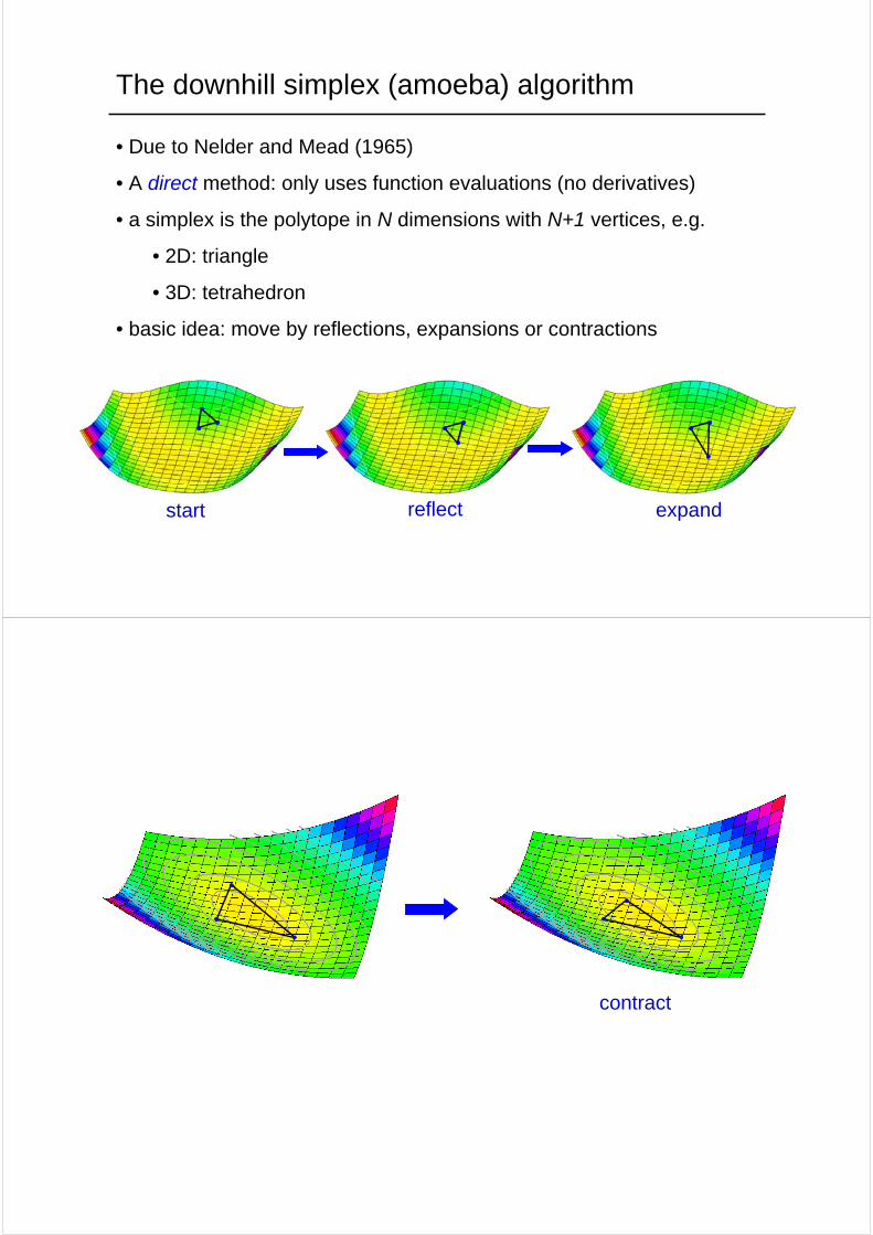
The downhill simplex (amoeba) algorithm

• Due to Nelder and Mead (1965)

• A direct method: only uses function evaluations (no derivatives)

• a simplex is the polytope in N dimensions with N+1 vertices, e.g.

• 2D: triangle

• 3D: tetrahedron

• basic idea: move by reflections, expansions or contractions

start reflect expand

contract

One iteration of the simplex algorithm

• Reorder the points so that f(xn+1) > f(x2) > f(x1) (i.e. xn+1 is the worst point).

• Generate a trial point xr by reflection

xr = x+ α(x− xn+1)where x =

¡Pi xi¢/(N + 1) is the centroid and α > 0. Compute f(xr), and there

are then 3 possibilities:

1. f(x1) < f(xr) < f(xn) (i.e. xr is neither the new best or worst point), replacexn+1 by xr.

2. f(xr) < f(x1) (i.e. xr is the new best point), then assume direction of reflectionis good and generate a new point by expansion

xe = xr+ β(xr − x)where β > 0. If f(xe) < f(xr) then replace xn+1 by xe, otherwise, the expansionhas failed, replace xn+1 by xr.

3. f(xr) > f(xn) then assume the polytope is too large and generate a new pointby contraction

xc = x+ γ(xn+1 − x)where γ (0 < γ < 1) is the contraction coefficient. If f(xc) < f(xn+1) then thecontraction has succeeded and replace xn+1 by xc, otherwise contract again.

Standard values are α = 1,β = 1, γ = 0.5.

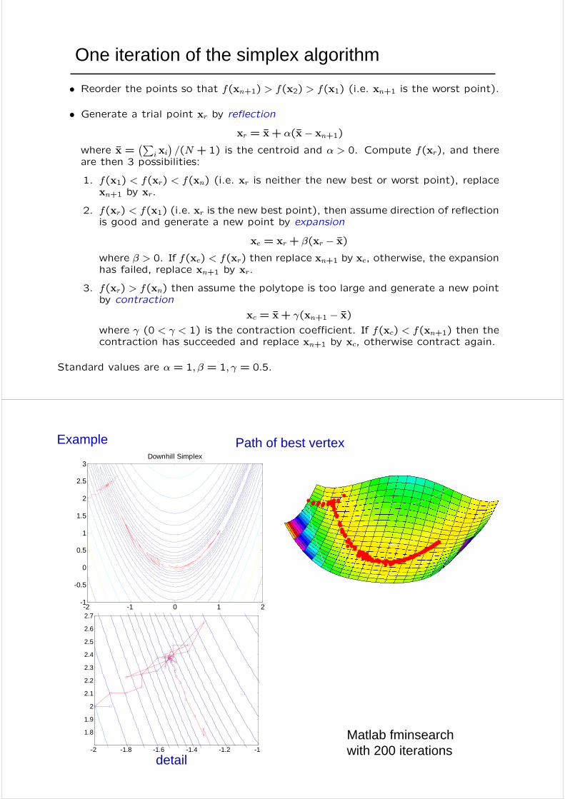
Example

-2 -1 0 1 2-1

-0.5

0

0.5

1

1.5

2

2.5

3Downhill Simplex

Path of best vertex

Matlab fminsearchwith 200 iterations-2 -1.8 -1.6 -1.4 -1.2 -1

1.8

1.9

2

2.1

2.2

2.3

2.4

2.5

2.6

2.7

detail

XX

YY

-1 0 1 2 3

-10

12

3

XX

YY

-1 0 1 2 3

-10

12

3

XX

YY

-1 0 1 2 3

-10

12

3

XX

YY

-1 0 1 2 3

-10

12

3

XX

YY

-1 0 1 2 3

-10

12

3

XX

YY

-1 0 1 2 3

-10

12

3

XX

YY

-1 0 1 2 3

-10

12

3

XX

YY

-1 0 1 2 3

-10

12

3

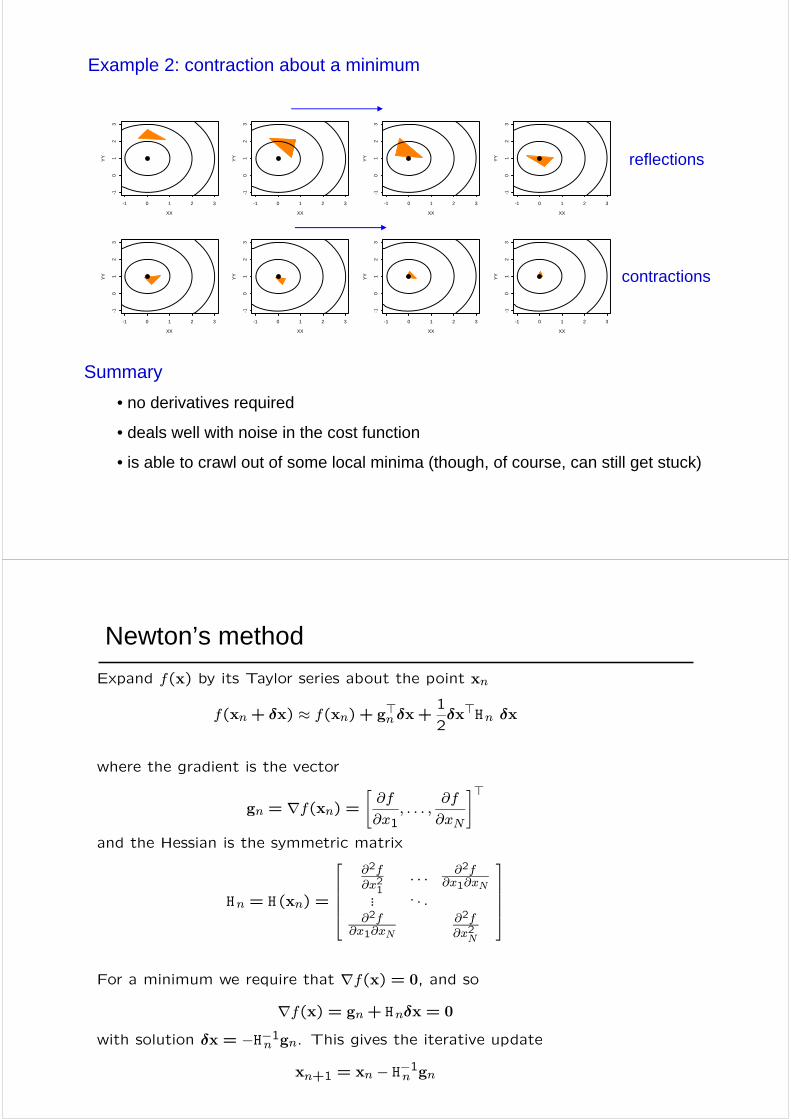
Example 2: contraction about a minimum

Summary

• no derivatives required

• deals well with noise in the cost function

• is able to crawl out of some local minima (though, of course, can still get stuck)

reflections

contractions

Newton’s method

Expand f(x) by its Taylor series about the point xn

f(xn+ δx) ≈ f(xn) + g>n δx+1

2δx>Hn δx

where the gradient is the vector

gn = ∇f(xn) ="∂f

∂x1, . . . ,

∂f

∂xN

#>and the Hessian is the symmetric matrix

Hn = H (xn) =

⎡⎢⎢⎢⎢⎣∂2f∂x21

. . . ∂2f∂x1∂xN

... . . .∂2f

∂x1∂xN∂2f∂x2N

⎤⎥⎥⎥⎥⎦

For a minimum we require that ∇f(x) = 0, and so

∇f(x) = gn+ Hnδx = 0

with solution δx = −H−1n gn. This gives the iterative update

xn+1 = xn − H−1n gn

• If f(x) is quadratic, then the solution is found in one step.

• The method has quadratic convergence (as in the 1D case).

• The solution δx = −H−1n gn is guaranteed to be a downhill direction.

• Rather than jump straight to the minimum, it is better to performa line minimization which ensures global convergence

xn+1 = xn − αnH−1n gn

• If H = I then this reduces to steepest descent.

xn+1 = xn − H−1n gn

Assume that H is positive definite (all eigenvalues greater than zero)

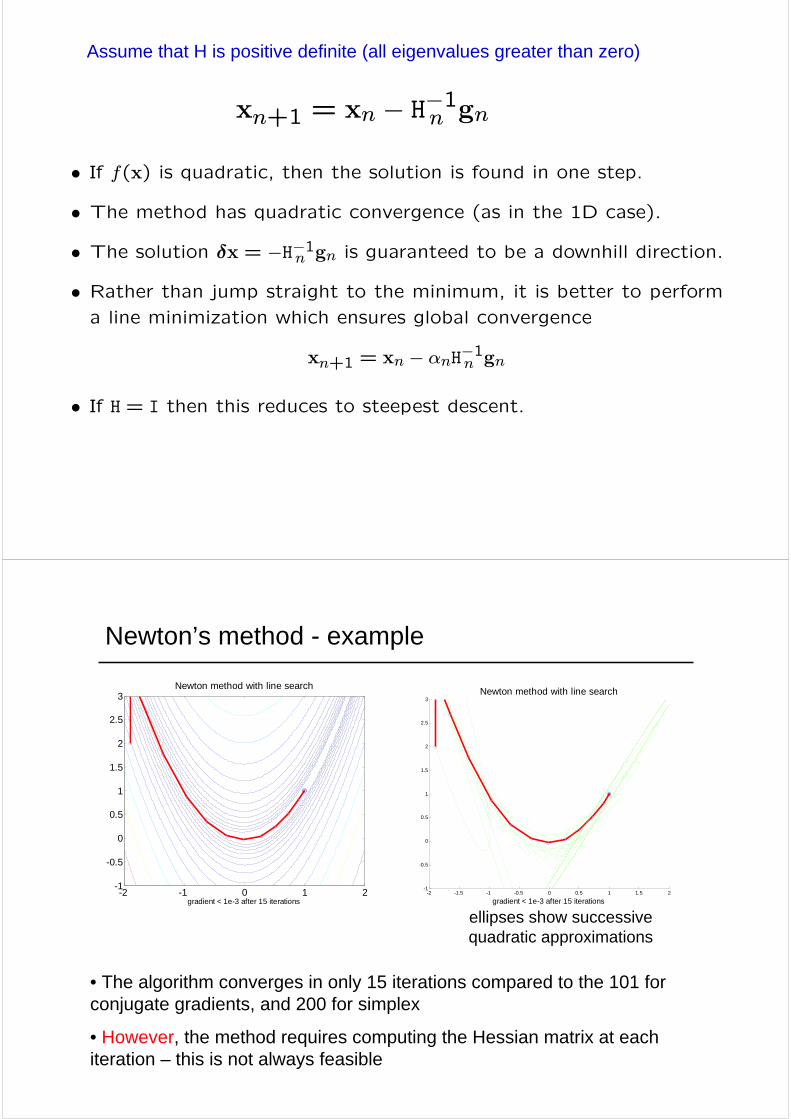
Newton’s method - example

-2 -1.5 -1 -0.5 0 0.5 1 1.5 2-1

-0.5

0

0.5

1

1.5

2

2.5

3Newton method with line search

gradient < 1e-3 after 15 iterations-2 -1 0 1 2

-1

-0.5

0

0.5

1

1.5

2

2.5

3Newton method with line search

gradient < 1e-3 after 15 iterations

ellipses show successive quadratic approximations

• The algorithm converges in only 15 iterations compared to the 101 for conjugate gradients, and 200 for simplex

• However, the method requires computing the Hessian matrix at each iteration – this is not always feasible

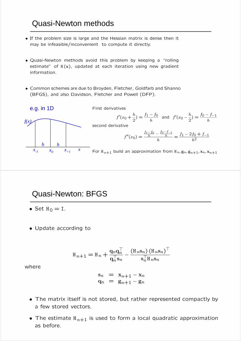
Quasi-Newton methods

• If the problem size is large and the Hessian matrix is dense then it

may be infeasible/inconvenient to compute it directly.

• Quasi-Newton methods avoid this problem by keeping a “rolling

estimate” of H (x), updated at each iteration using new gradient

information.

• Common schemes are due to Broyden, Fletcher, Goldfarb and Shanno(BFGS), and also Davidson, Fletcher and Powell (DFP).

First derivatives

f 0(x0 +h

2) =

f1 − f0h

and f 0(x0 −h

2) =

f0 − f−1h

second derivative

f 00(x0) =f1−f0h − f0−f−1

h

h=f1 − 2f0 + f−1

h2

For Hn+1 build an approximation from Hn, gn, gn+1,xn,xn+1

e.g. in 1D

xx-1 x+1x0

h h

f(x)

Quasi-Newton: BFGS

• Set H0 = I.

• Update according to

Hn+1 = Hn+qnq>nq>n sn

− (Hnsn) (Hnsn)>

s>n Hnsnwhere

sn = xn+1 − xnqn = gn+1 − gn

• The matrix itself is not stored, but rather represented compactly bya few stored vectors.

• The estimate Hn+1 is used to form a local quadratic approximation

as before.

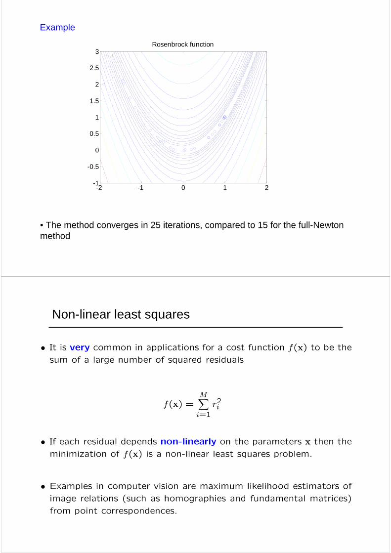
Example

-2 -1 0 1 2-1

-0.5

0

0.5

1

1.5

2

2.5

3Rosenbrock function

• The method converges in 25 iterations, compared to 15 for the full-Newton method

Non-linear least squares

• It is very common in applications for a cost function f(x) to be thesum of a large number of squared residuals

f(x) =MXi=1

r2i

• If each residual depends non-linearly on the parameters x then theminimization of f(x) is a non-linear least squares problem.

• Examples in computer vision are maximum likelihood estimators of

image relations (such as homographies and fundamental matrices)

from point correspondences.

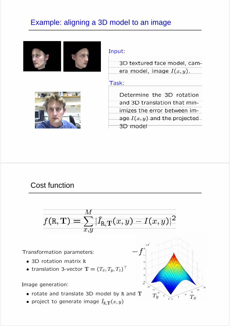
Example: aligning a 3D model to an image

Transformation parameters:

• 3D rotation matrix R

• translation 3-vector T = (Tx, Ty, Tz)>

Image generation:

• rotate and translate 3D model by R and T

• project to generate image IR,T(x, y)

Cost function

TxTy

−f

J>

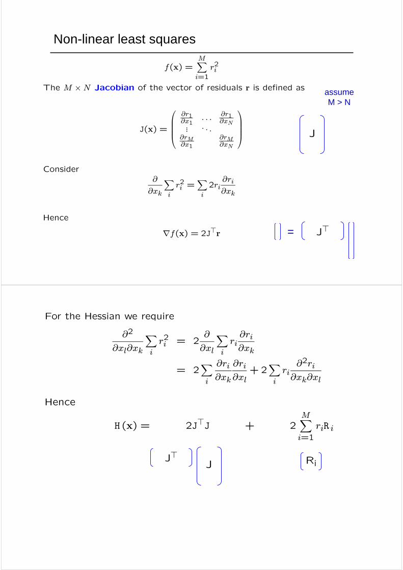
f(x) =MXi=1

r2i

The M ×N Jacobian of the vector of residuals r is defined as

J(x) =

⎛⎜⎜⎜⎝∂r1∂x1

. . . ∂r1∂xN... . . .

∂rM∂x1

∂rM∂xN

⎞⎟⎟⎟⎠

Consider∂

∂xk

Xi

r2i =Xi

2ri∂ri∂xk

Hence

∇f(x) = 2J>r

Non-linear least squares

assume M > N

J

=

For the Hessian we require

∂2

∂xl∂xk

Xi

r2i = 2∂

∂xl

Xi

ri∂ri∂xk

= 2Xi

∂ri∂xk

∂ri∂xl

+2Xi

ri∂2ri

∂xk∂xl

Hence

H (x) = 2J>J + 2MXi=1

riR i

J>J Ri

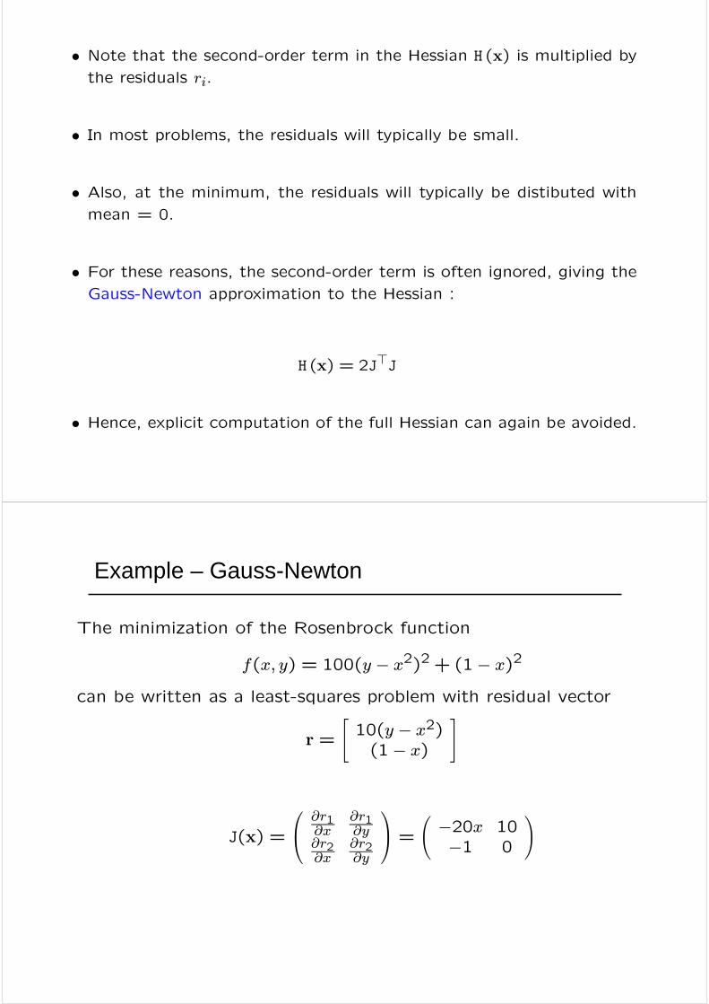
• Note that the second-order term in the Hessian H (x) is multiplied by

the residuals ri.

• In most problems, the residuals will typically be small.

• Also, at the minimum, the residuals will typically be distibuted withmean = 0.

• For these reasons, the second-order term is often ignored, giving the

Gauss-Newton approximation to the Hessian :

H (x) = 2J>J

• Hence, explicit computation of the full Hessian can again be avoided.

Example – Gauss-Newton

The minimization of the Rosenbrock function

f(x, y) = 100(y − x2)2 + (1− x)2

can be written as a least-squares problem with residual vector

r =

"10(y − x2)(1− x)

#

J(x) =

⎛⎝ ∂r1∂x

∂r1∂y

∂r2∂x

∂r2∂y

⎞⎠ = Ã−20x 10−1 0

!

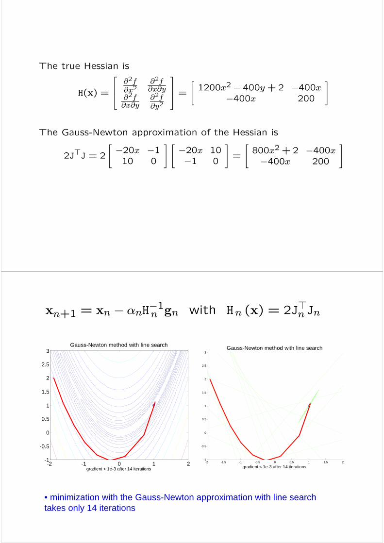
The true Hessian is

H(x) =

⎡⎢⎣ ∂2f∂x2

∂2f∂x∂y

∂2f∂x∂y

∂2f∂y2

⎤⎥⎦ = "1200x2 − 400y+2 −400x

−400x 200

#

The Gauss-Newton approximation of the Hessian is

2J>J = 2

"−20x −110 0

# "−20x 10−1 0

#=

"800x2 + 2 −400x−400x 200

#

-2 -1.5 -1 -0.5 0 0.5 1 1.5 2-1

-0.5

0

0.5

1

1.5

2

2.5

3Gauss-Newton method with line search

gradient < 1e-3 after 14 iterations-2 -1 0 1 2

-1

-0.5

0

0.5

1

1.5

2

2.5

3Gauss-Newton method with line search

gradient < 1e-3 after 14 iterations

• minimization with the Gauss-Newton approximation with line search takes only 14 iterations

xn+1 = xn − αnH−1n gn with Hn (x) = 2J>n Jn

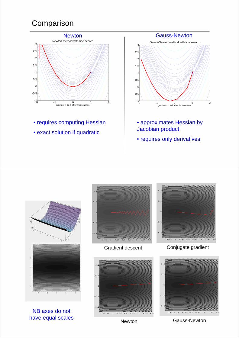
Comparison

-2 -1 0 1 2-1

-0.5

0

0.5

1

1.5

2

2.5

3Gauss-Newton method with line search

gradient < 1e-3 after 14 iterations-2 -1 0 1 2

-1

-0.5

0

0.5

1

1.5

2

2.5

3Newton method with line search

gradient < 1e-3 after 15 iterations

Newton Gauss-Newton

• requires computing Hessian

• exact solution if quadratic

• approximates Hessian by Jacobian product

• requires only derivatives

Conjugate gradient

Gauss-Newton

Gradient descent

Newton

NB axes do not have equal scales

Conjugate gradient

Gauss-Newton (no line search)

Gradient descent

Newton