Lecture 2 Today: Statistical Review cont’d: Expected value, variance and covariance rules Sampling and estimators Unbiasedness and efficiency Sample equivalents

Lecture 2

Today:• Statistical Review cont’d:

• Expected value, variance and covariance rules• Sampling and estimators• Unbiasedness and efficiency• Sample equivalents of variance, covariance and correlation

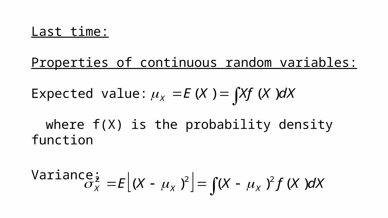
Last time:

Properties of discrete random variables:

Expected value:

Variance:

n

iiinnX pxpxpxXE

111 ...)(

i

n

iXinXnX

X

pxpxpx

XE

1

221

2

22

)()(...)(

)(

Last time:

Properties of continuous random variables:

Expected value:

where f(X) is the probability density function

Variance:

dXXXfXEX )()(

dXXfXXE XXX )()()( 222

© Christopher Dougherty 1999–2006

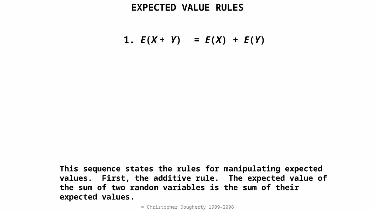
1. E(X + Y) = E(X) + E(Y)

EXPECTED VALUE RULES

This sequence states the rules for manipulating expected values. First, the additive rule. The expected value of the sum of two random variables is the sum of their expected values.


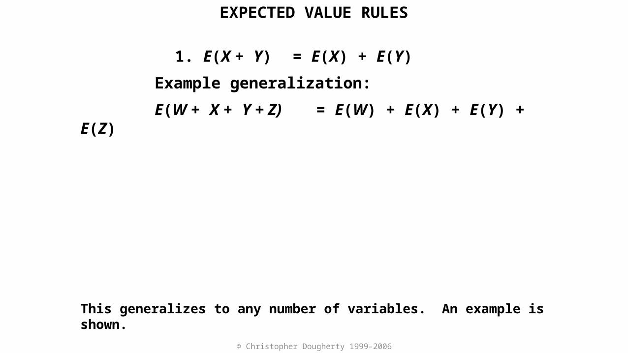
1. E(X + Y) = E(X) + E(Y)

Example generalization:

E(W + X + Y + Z) = E(W) + E(X) + E(Y) + E(Z)

This generalizes to any number of variables. An example is shown.



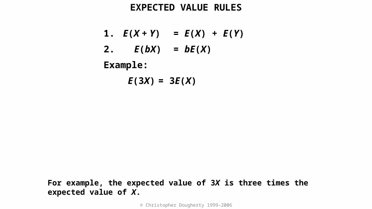
1. E(X + Y) = E(X) + E(Y)

2. E(bX) = bE(X)


The second rule is the multiplicative rule. The expected value of (a variable multiplied by a constant) is equal to the constant multiplied by the expected value of the variable.


1. E(X + Y) = E(X) + E(Y)

2. E(bX) = bE(X)

Example:

E(3X) = 3E(X)


For example, the expected value of 3X is three times the expected value of X.


1. E(X + Y) = E(X) + E(Y)

2. E(bX) = bE(X)

3. E(b) = b


Finally, the expected value of a constant is just the constant. Of course this is obvious.


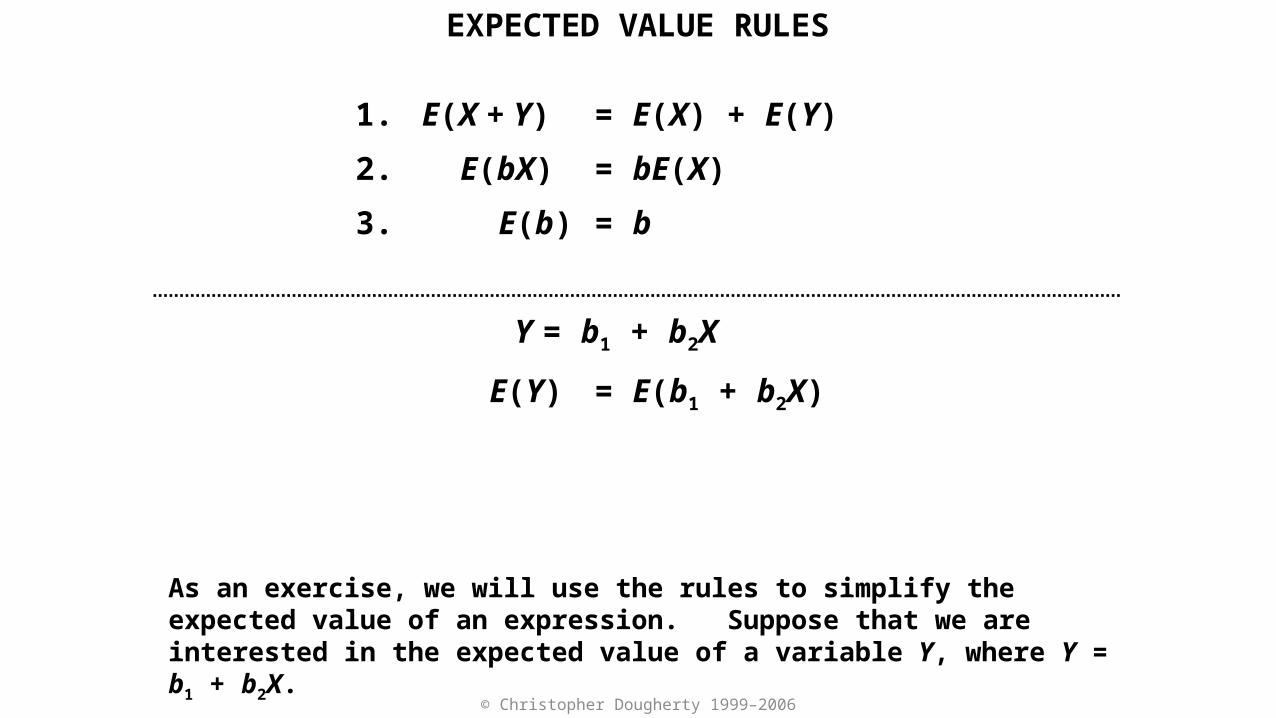
1. E(X + Y) = E(X) + E(Y)

2. E(bX) = bE(X)

3. E(b) = b

Y = b1 + b2X

E(Y) = E(b1 + b2X)


As an exercise, we will use the rules to simplify the expected value of an expression. Suppose that we are interested in the expected value of a variable Y, where Y = b1 + b2X.


1. E(X + Y) = E(X) + E(Y)

2. E(bX) = bE(X)

3. E(b) = b

Y = b1 + b2X

E(Y) = E(b1 + b2X)

= E(b1) + E(b2X)


We use the first rule to break up the expected value into its two components.


1. E(X + Y) = E(X) + E(Y)

2. E(bX) = bE(X)

3. E(b) = b

Y = b1 + b2X

E(Y) = E(b1 + b2X)

= E(b1) + E(b2X)

= b1 + b2E(X)

Then we use the second rule to replace E(b2X) by b2E(X) and the third rule to simplify E(b1) to just b1. This is as far as we can go in this example.



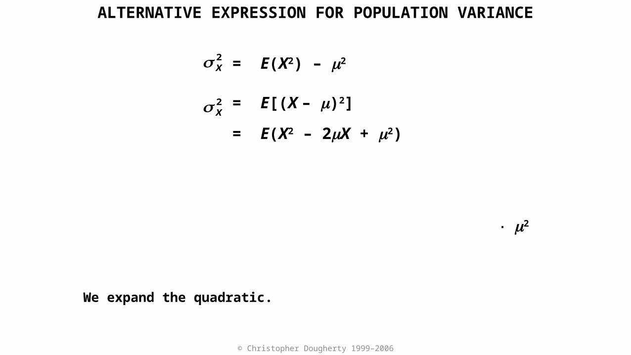
ALTERNATIVE EXPRESSION FOR POPULATION VARIANCE

This sequence derives an alternative expression for the population variance of a random variable. It provides an opportunity for practising the use of the expected value rules.

2X

2X = E(X2) – m2

= E[(X – m)2]

= E(X2 – 2mX + m2)

= E(X2) + E(–2mX) + E(m2)

= E(X2) – 2mE(X) + m2

= E(X2) – 2m2 + m2 = E(X2) – m2



We start with the definition of the population variance of X.

2X

2X = E(X2) – m2

= E[(X – m)2]

= E(X2 – 2mX + m2)

= E(X2) + E(–2mX) + E(m2)

= E(X2) – 2mE(X) + m2

= E(X2) – 2m2 + m2 = E(X2) – m2



We expand the quadratic.

2X

2X = E(X2) – m2

= E[(X – m)2]

= E(X2 – 2mX + m2)

= E(X2) + E(–2mX) + E(m2)

= E(X2) – 2mE(X) + m2

= E(X2) – 2m2 + m2 = E(X2) – m2



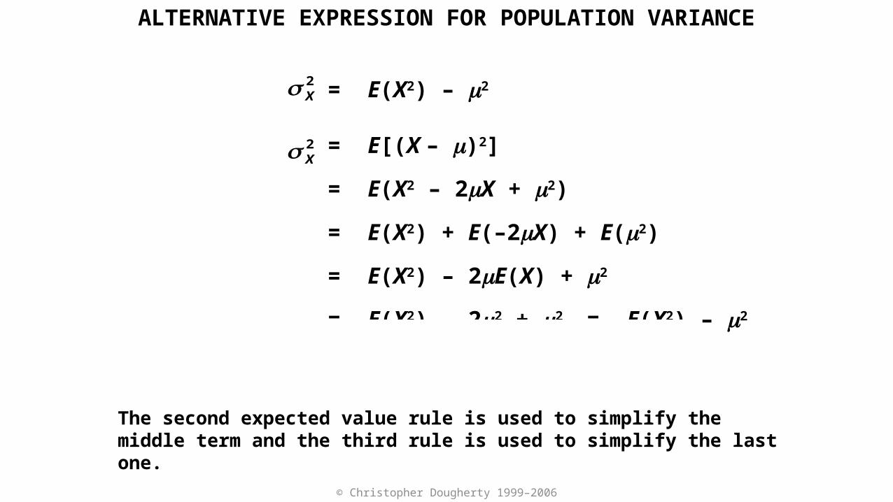
Now the first expected value rule is used to decompose the expression into three separate expected values.

2X

2X = E(X2) – m2

= E[(X – m)2]

= E(X2 – 2mX + m2)

= E(X2) + E(–2mX) + E(m2)

= E(X2) – 2mE(X) + m2

= E(X2) – 2m2 + m2 = E(X2) – m2



The second expected value rule is used to simplify the middle term and the third rule is used to simplify the last one.

2X

2X = E(X2) – m2

= E[(X – m)2]

= E(X2 – 2mX + m2)

= E(X2) + E(–2mX) + E(m2)

= E(X2) – 2mE(X) + m2

= E(X2) – 2m2 + m2 = E(X2) – m2



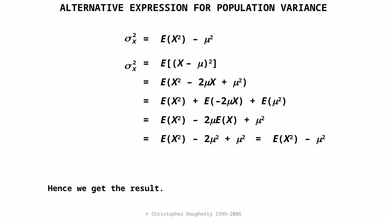
The middle term is rewritten, using the fact that E(X) and mX are just different ways of writing the population mean of X.

2X

2X = E(X2) – m2

= E[(X – m)2]

= E(X2 – 2mX + m2)

= E(X2) + E(–2mX) + E(m2)

= E(X2) – 2mE(X) + m2

= E(X2) – 2m2 + m2 = E(X2) – m2


= E(X2) – m2

= E[(X – m)2]

= E(X2 – 2mX + m2)

= E(X2) + E(–2mX) + E(m2)

= E(X2) – 2mE(X) + m2

= E(X2) – 2m2 + m2 = E(X2) – m2

Hence we get the result.


2X

2X


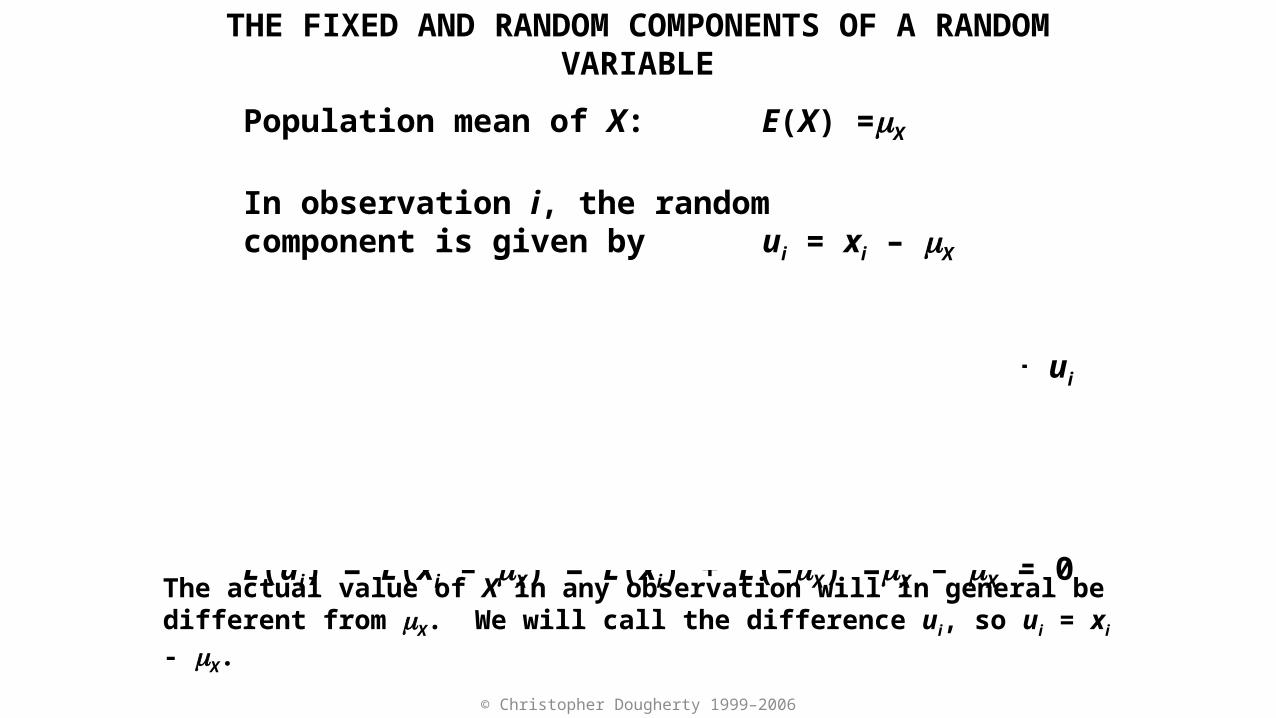
THE FIXED AND RANDOM COMPONENTS OF A RANDOM VARIABLE

In this short sequence we shall decompose a random variable X into its fixed and random components. Let the population mean of X be mX.

Population mean of X: E(X) =mX

In observation i, the randomcomponent is given by ui = xi – mX

Hence xi can be decomposedinto fixed and random components: xi = mX + ui

Note that the expected valueof ui is zero:

E(ui) = E(xi – mX) = E(xi) + E(–mX) =mX – mX = 0



The actual value of X in any observation will in general be different from mX. We will call the difference ui, so ui = xi - mX.








Re-arranging this equation, we can write xi as the sum of its fixed component, mX, which is the same for all observations, and its random component, ui.












The expected value of the random component is zero. It does not systematically tend to increase or decrease X. It just makes it deviate from its population mean.



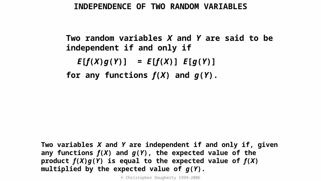
Two random variables X and Y are said to beindependent if and only if

E[f(X)g(Y)] = E[f(X)] E[g(Y)]

for any functions f(X) and g(Y).

INDEPENDENCE OF TWO RANDOM VARIABLES

Two variables X and Y are independent if and only if, given any functions f(X) and g(Y), the expected value of the product f(X)g(Y) is equal to the expected value of f(X) multiplied by the expected value of g(Y).


Two random variables X and Y are said to beindependent if and only if

E[f(X)g(Y)] = E[f(X)] E[g(Y)]

for any functions f(X) and g(Y).

Special case: if X and Y are independent,

E(XY) = E(X) E(Y)

INDEPENDENCE OF TWO RANDOM VARIABLES

As a special case, the expected value of XY is equal to the expected value of X multiplied by the expected value of Y if and only if X and Y are independent.


Covariance

The covariance of two random variables X and Y, often written sXY, is defined to be the expected value of the product of their deviations from their population means.

))(( ),cov( YXXY YXEYX

COVARIANCE, COVARIANCE AND VARIANCE RULES, AND CORRELATION


000

)()()()(

)()())((

YYXX

YX

YXYX

EYEEXE

YEXEYXE

If two variables are independent, their covariance is zero.

To show this, start by rewriting the covariance as the product of the expected values of its factors.

We are allowed to do this because (and only because) X and Y are independent (see the earlier sequence on independence.

Covariance




000

)()()()(

)()())((

YYXX

YX

YXYX

EYEEXE

YEXEYXE


The expected values of both factors are zero because E(X) = mX and E(Y) = mY. E(mX) = mX and E(mY) = mY because mX and mY are constants. Thus the covariance is zero.

Covariance



There are some rules that follow in a perfectly straightforward way from the definition of covariance, and since they are going to be used frequently in later chapters it is worthwhile establishing them immediately. First, the addition rule.

Covariance rules

1. If Y = V + W,cov(X, Y) = cov(X, V) + cov(X,W).

2. If Y = bZ, where b is a constantcov(X, Y) = bcov(X, Z)

3. If Y = b, where b is a constant,cov(X, Y) = 0



Next, the multiplication rule, for cases where a variable is multiplied by a constant.

Covariance rules





© Christopher Dougherty 1999–2006 7

Finally, a primitive rule that is often useful.

Covariance rules






The proofs of the rules are straightforward. In each case the proof starts with the definition of cov(X, Y).

Covariance rules


Proof:

Since Y = V + W, mY = mV + mW

).,(cov),(cov

][][

),(cov

WXVX

WXVXE

WVXE

YXEYX

WXVX

WVX

YX




We now substitute for Y and re-arrange.

Covariance rules


Proof:


).,(cov),(cov

][][

),(cov

WXVX

WXVXE

WVXE

YXEYX

WXVX

WVX

YX



This gives us the result.

Covariance rules


Proof:


).,(cov),(cov

][][

),(cov

WXVX

WXVXE

WVXE

YXEYX

WXVX

WVX

YX



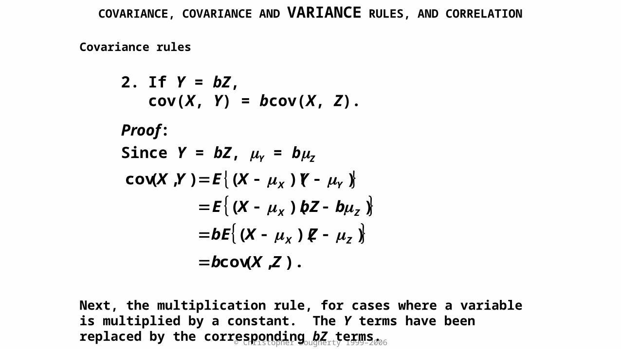
Next, the multiplication rule, for cases where a variable is multiplied by a constant. The Y terms have been replaced by the corresponding bZ terms.

Covariance rules

2. If Y = bZ,cov(X, Y) = bcov(X, Z).

Proof:

Since Y = bZ, mY = bmZ

).,(cov

))((

))((

))((),(cov

ZXb

ZXbE

bbZXE

YXEYX

ZX

ZX

YX



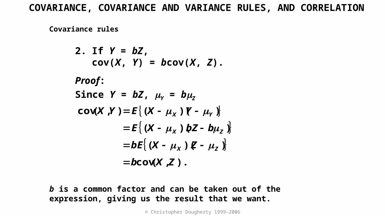
b is a common factor and can be taken out of the expression, giving us the result that we want.

Covariance rules

2. If Y = bZ,cov(X, Y) = bcov(X, Z).

Proof:

Since Y = bZ, mY = bmZ

).,(cov

))((

))((

))((),(cov

ZXb

ZXbE

bbZXE

YXEYX

ZX

ZX

YX



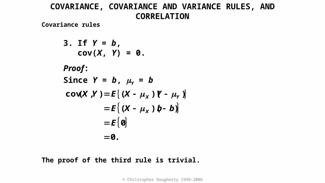
The proof of the third rule is trivial.

Covariance rules

3. If Y = b,cov(X, Y) = 0.

Proof:

Since Y = b, mY = b

.0

0

))((

))((),(cov

E

bbXE

YXEYX

X

YX



Corresponding to the covariance rules, there are parallel rules for variances. First the addition rule.

Variance rules

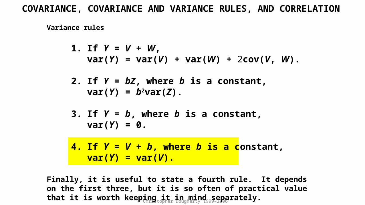
1. If Y = V + W,var(Y) = var(V) + var(W) + 2cov(V, W).

2. If Y = bZ, where b is a constant,var(Y) = b2var(Z).

3. If Y = b, where b is a constant,var(Y) = 0.

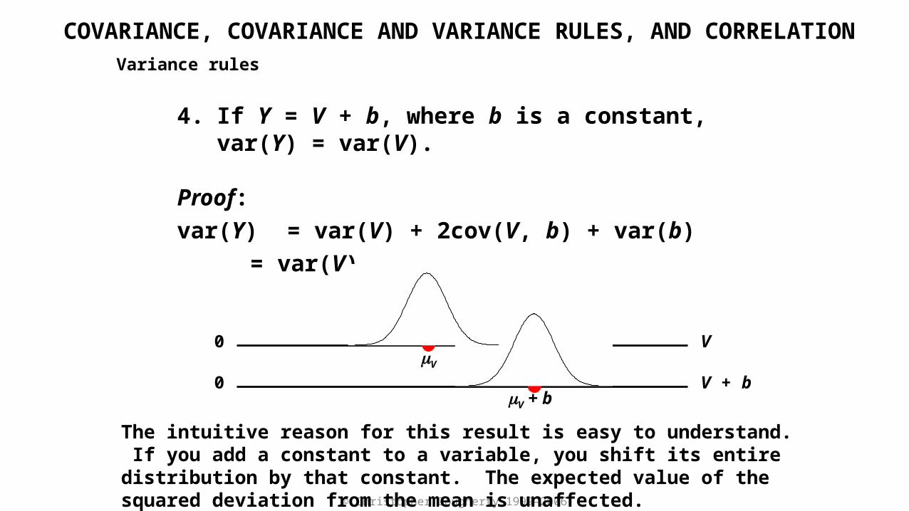
4. If Y = V + b, where b is a constant,var(Y) = var(V).



Next, the multiplication rule, for cases where a variable is multiplied by a constant.

Variance rules







A third rule to cover the special case where Y is a constant.

Variance rules






Finally, it is useful to state a fourth rule. It depends on the first three, but it is so often of practical value that it is worth keeping it in mind separately.

Variance rules







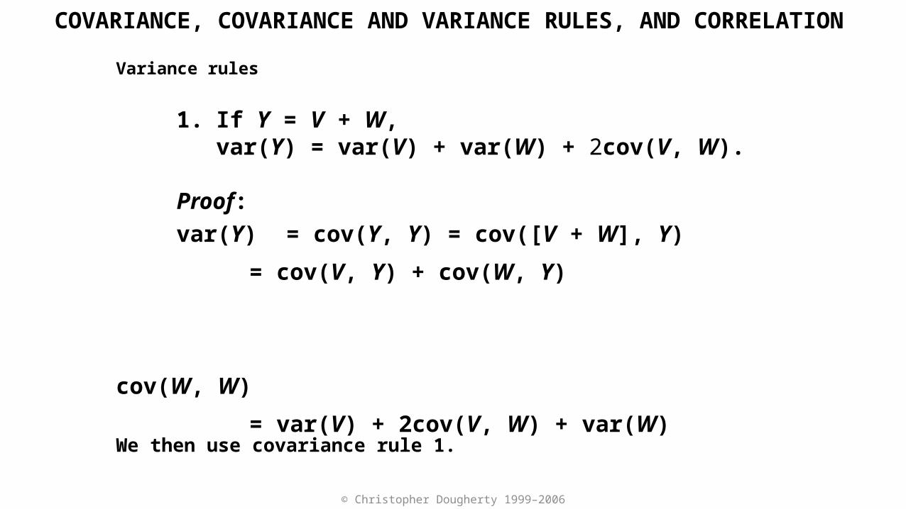
The proofs of these rules can be derived from the results for covariances, noting that the variance of Y is equivalent to the covariance of Y with itself.

Variance rules


Proof:

var(Y) = cov(Y, Y) = cov([V + W], Y)

= cov(V, Y) + cov(W, Y)

= cov(V, [V + W]) + cov(W, [V + W])

= cov(V, V) + cov(V,W) + cov(W, V) + cov(W, W)

= var(V) + 2cov(V, W) + var(W)

).,(cov

))((

)()(var 2

XX

XXE

XEX

XX

X



We start by replacing one of the Y arguments by V + W.

Variance rules


Proof:



= cov(V, [V + W]) + cov(W, [V + W])





We then use covariance rule 1.

Variance rules


Proof:



= cov(V, [V + W]) + cov(W, [V + W])





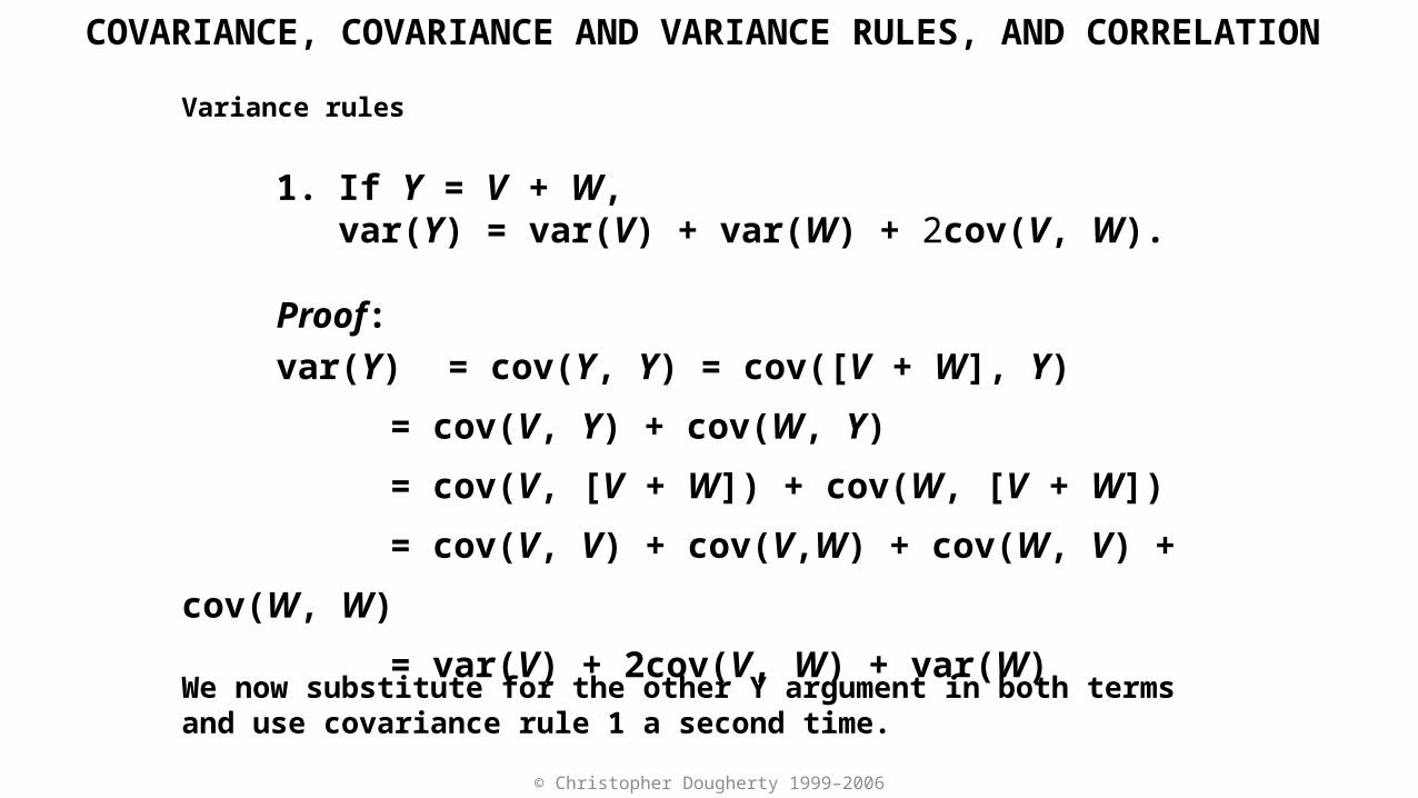
We now substitute for the other Y argument in both terms and use covariance rule 1 a second time.

Variance rules


Proof:



= cov(V, [V + W]) + cov(W, [V + W])





This gives us the result. Note that the order of the arguments does not affect a covariance expression and hence cov(W, V) is the same as cov(V, W).

Variance rules


Proof:



= cov(V, [V + W]) + cov(W, [V + W])





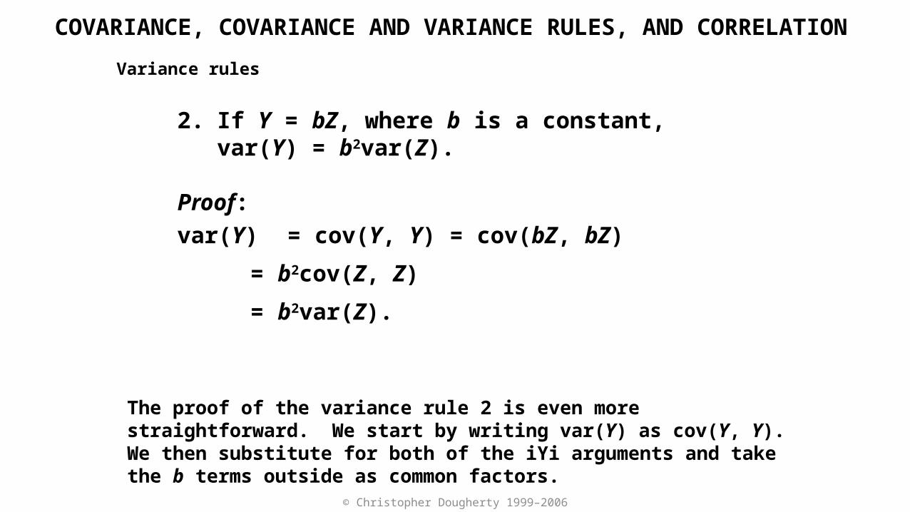
The proof of the variance rule 2 is even more straightforward. We start by writing var(Y) as cov(Y, Y). We then substitute for both of the iYi arguments and take the b terms outside as common factors.

Variance rules


Proof:

var(Y) = cov(Y, Y) = cov(bZ, bZ)

= b2cov(Z, Z)

= b2var(Z).



The third rule is trivial. We make use of covariance rule 3. Obviously if a variable is constant, it has zero variance.

Variance rules


Proof:

var(Y) = cov(b, b) = 0.



The fourth variance rule starts by using the first. The second term on the right side is zero by covariance rule 3. The third is also zero by variance rule 3.

Variance rules


Proof:

var(Y) = var(V) + 2cov(V, b) + var(b)

= var(V)



The intuitive reason for this result is easy to understand. If you add a constant to a variable, you shift its entire distribution by that constant. The expected value of the squared deviation from the mean is unaffected.

Variance rules


Proof:

var(Y) = var(V) + 2cov(V, b) + var(b)

= var(V)

0

0 V + b

VmV

mV + b



cov(X, Y) is unsatisfactory as a measure of association between two variables X and Y because it depends on the units of measurement of X and Y.

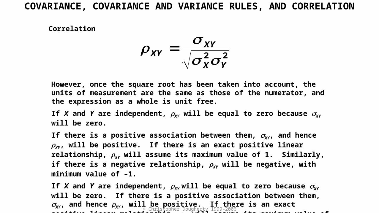
A better measure of association is the population correlation coefficient because it is dimensionless. The numerator possesses the units of measurement of both X and Y.

The variances of X and Y in the denominator possess the squared units of measurement of those variables.

Correlation

22YX

XYXY



However, once the square root has been taken into account, the units of measurement are the same as those of the numerator, and the expression as a whole is unit free.

If X and Y are independent, rXY will be equal to zero because sXY will be zero.

If there is a positive association between them, sXY, and hence rXY, will be positive. If there is an exact positive linear relationship, rXY will assume its maximum value of 1. Similarly, if there is a negative relationship, rXY will be negative, with minimum value of –1.

If X and Y are independent, rXY will be equal to zero because sXY will be zero. If there is a positive association between them, sXY, and hence rXY, will be positive. If there is an exact positive linear relationship, rXY will assume its maximum value of 1. Similarly, if there is a negative relationship, rXY will be negative, with minimum value of –1.

Correlation

22YX

XYXY



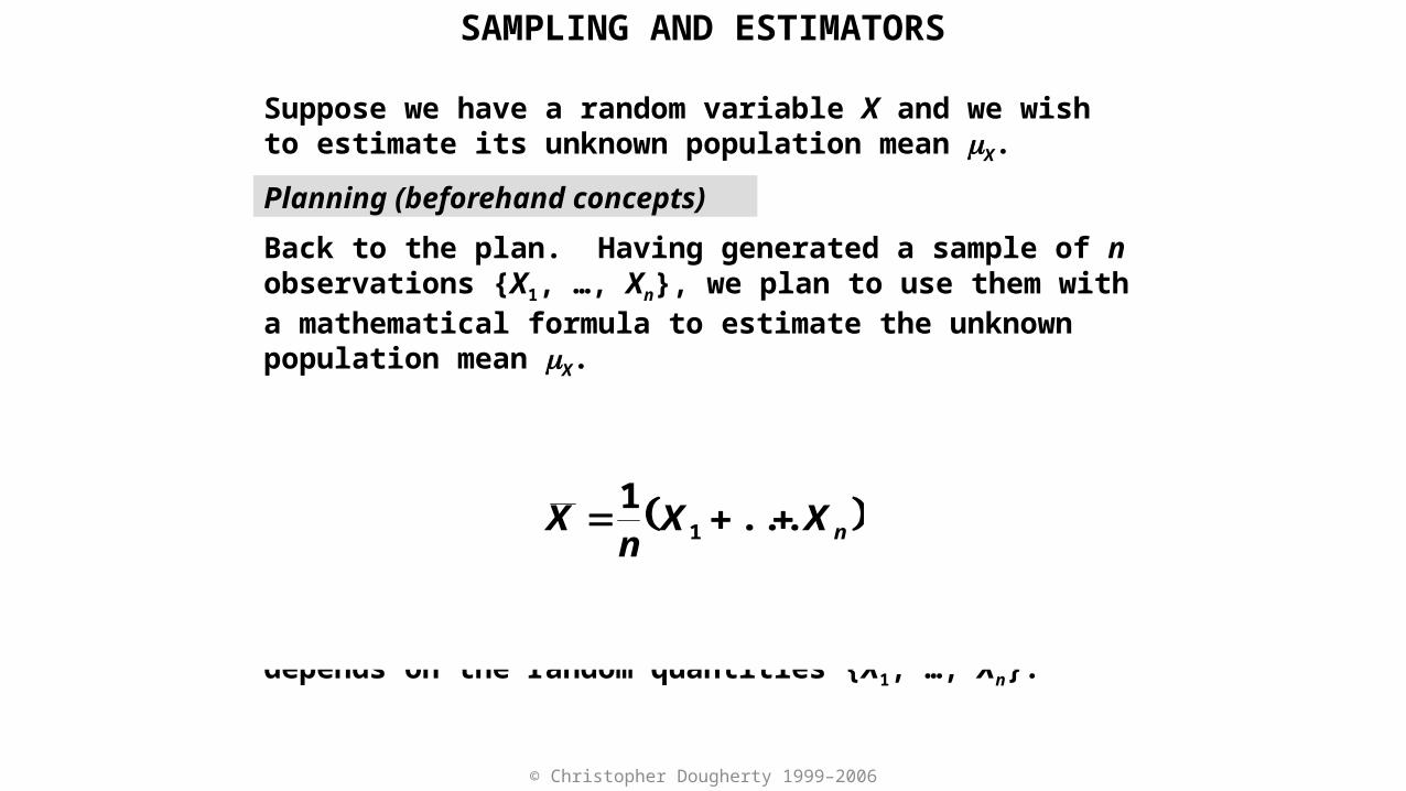
Suppose we have a random variable X and we wish to estimate its unknown population mean mX.

Planning (beforehand concepts)

Our first step is to take a sample of n observations {X1, …, Xn}.

Before we take the sample, while we are still at the planning stage, the Xi are random quantities. We know that they will be generated randomly from the distribution for X, but we do not know their values in advance.

So now we are thinking about random variables on two levels: the random variable X, and its random sample components.

SAMPLING AND ESTIMATORS




Our first step is to take a sample of n observations {X1, …, Xn}.

Before we take the sample, while we are still at the planning stage, the Xi are random quantities. We know that they will be generated randomly from the distribution for X, but we do not know their values in advance.

So now we are thinking about random variables on two levels: the random variable X, and its random sample components.




Realization (afterwards concepts)

Once we have taken the sample we will have a set of numbers {x1, …, xn}.

This is called by statisticians a realization. The lower case is to emphasize that these are numbers, not variables.





Back to the plan. Having generated a sample of n observations {X1, …, Xn}, we plan to use them with a mathematical formula to estimate the unknown population mean mX.

This formula is known as an estimator. In this context, the standard (but not only) estimator is the sample mean

An estimator is a random variable because it depends on the random quantities {X1, …, Xn}.

nXXn

X ...1

1





Back to the plan. Having generated a sample of n observations {X1, …, Xn}, we plan to use them with a mathematical formula to estimate the unknown population mean mX.

This formula is known as an estimator. In this context, the standard (but not only) estimator is the sample mean

An estimator is a random variable because it depends on the random quantities {X1, …, Xn}.

nXXn

X ...1

1




Realization (afterwards concepts)

The actual number that we obtain, given the realization {x1, …, xn}, is known as our estimate.



probability density

function of X

mX

XmX

X

probability density

function of X

We will see why these distinctions are useful and important in a comparison of the distributions of X and X. We will start by showing that X has the same mean as X.



XXX

n

n

n

n

XEXEn

XXEn

XXn

EXE

...1

...1

...1

...1

1

1

1

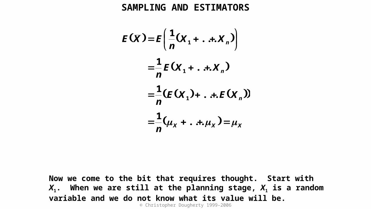
We start by replacing X by its definition and then using expected value rule 2 to take 1/n out of the expression as a common factor.



XXX

n

n

n

n

XEXEn

XXEn

XXn

EXE

...1

...1

...1

...1

1

1

1

Next we use expected value rule 1 to replace the expectation of a sum with a sum of expectations.



XXX

n

n

n

n

XEXEn

XXEn

XXn

EXE

...1

...1

...1

...1

1

1

1

Now we come to the bit that requires thought. Start with X1. When we are still at the planning stage, X1 is a random variable and we do not know what its value will be.



XXX

n

n

n

n

XEXEn

XXEn

XXn

EXE

...1

...1

...1

...1

1

1

1

All we know is that it will be generated randomly from the distribution of X. The expected value of X1, as a beforehand concept, will therefore be mX. The same is true for all the other sample components, thinking about them beforehand. Hence we write this line.



Thus we have shown that the mean of the distribution of X is mX.

XXX

n

n

n

n

XEXEn

XXEn

XXn

EXE

...1

...1

...1

...1

1

1

1



We will next demonstrate that the variance of the distribution of X is smaller than that of X, as depicted in the diagram.

probability density

function of X

mX

XmX

X

probability density

function of X



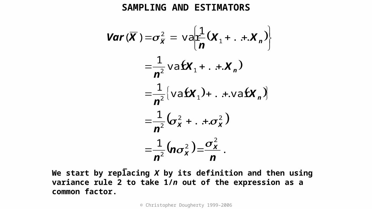
.1

...1

var...var1

...var1

...1

var)(

22

2

222

12

12

12

nn

n

n

XXn

XXn

XXn

XVar

XX

XX

n

n

nX

We start by replacing X by its definition and then using variance rule 2 to take 1/n out of the expression as a common factor.



.1

...1

var...var1

...var1

...1

var

22

2

222

12

12

12

nn

n

n

XXn

XXn

XXn

XX

XX

n

n

nX

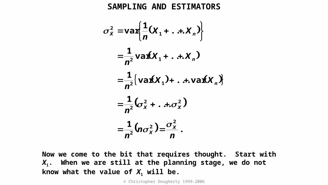
Next we use variance rule 1 to replace the variance of a sum with a sum of variances. In principle there are many covariance terms as well, but they are zero if we assume that the sample values are generated independently.



.1

...1

var...var1

...var1

...1

var

22

2

222

12

12

12

nn

n

n

XXn

XXn

XXn

XX

XX

n

n

nX

Now we come to the bit that requires thought. Start with X1. When we are still at the planning stage, we do not know what the value of X1 will be.



.1

...1

var...var1

...var1

...1

var

22

2

222

12

12

12

nn

n

n

XXn

XXn

XXn

XX

XX

n

n

nX

All we know is that it will be generated randomly from the distribution of X. The variance of X1, as a beforehand concept, will therefore be sX. The same is true for all the other sample components, thinking about them beforehand. Hence we write this line.

2



.1

...1

var...var1

...var1

...1

var

22

2

222

12

12

12

nn

n

n

XXn

XXn

XXn

XX

XX

n

n

nX

Thus we have demonstrated that the variance of the sample mean is equal to the variance of X divided by n, a result with which you will be familiar from your statistics course.


Documents

Lecture 2 Today: Statistical Review cont’d: Expected value, variance and covariance rules Sampling and estimators Unbiasedness and efficiency Sample equivalents